Numerical Evaluation of the Effectiveness of the Use of Endplates in Front Wings in Formula One Cars under Multiple Track Operating Conditions

Abstract

The last change in the technical regulations of Formula One that came into force in 2022 brought with it significant changes in the aerodynamics of the vehicle; among these, those made to the front wing stand out since the wing was changed to a more straightforward shape with fewer parts but with no less efficiency. The reduction in its components suggests that if one part were to suffer damage or break down, the efficiency of the entire front wing would be affected; however, from 2022 to date, there have been occasions in which the cars have continued running on the track despite losing some of the endplates. This research seeks to understand the endplates’ impact on the front wing through a series of CFD simulations using the k-ω SST turbulence model. To determine efficiency, the aerodynamic forces generated on the vehicle’s front wing, suspension, and front wheels were compared in two different operating situations using a model with the front wing in good condition and another in which the endplates were removed. The first case study simulated a straight line at a maximum speed where the Downforce is reduced by 2.716% while the Drag and Yaw increase by 7.092% and 96.332%, respectively, when the model does not have endplates. On the other hand, the second case study was the passage through a curve with a decrease of 17.707% in Downforce, 6.532% in Drag, and 22.200% in Yaw.

1. Introduction

In motorsports, Formula One is considered the most important category where the best drivers compete aboard the best cars in the world. Over time, the teams participating in this championship have found it necessary to adapt their vehicles to changes in regulations; these changes are justified since they seek to provide the teams with security and leave them on equal terms, always considering technological innovations and new design trends. The FIA (Fédération Internationale de l’Automobile), the entity in charge of regulating this championship, plays a crucial role in setting these regulations and ensuring fair competition [1,2].

In car racing, it is essential to provide vehicles with good aerodynamics to provide drivers with a stable vehicle with good performance that is not only competitive but can also win races. This objective can be achieved if the car can generate sufficient Downforce when accelerating in a straight area of the circuit or when cornering, since in this way, the vehicle’s grip on the track is improved [3,4]. The front wing is responsible for providing the vehicle with at least a quarter of the total Downforce necessary to keep the vehicle on track [5]. Since these devices were introduced to Formula One in the 1960s, they have become the most crucial aerodynamic element of the single-seater bodywork. As a result, the correct design of a front wing can make a big difference in the level of competitiveness of the vehicles [6,7].

Several authors have researched the importance, operation, and optimizations of the design of front wings for competitive vehicles. Castro et al. [8] focused their research on designing and evaluating a new front wing model for the change in technical regulations of Formula One in 2022. Basso et al. [9] analyzed the aerodynamic effects generated by the use of gurney flaps on front wings. Gere-Gurky et al. [10] described the aerodynamic behavior of the car’s front wings used in the 2018 and 2019 Formula One seasons. Petrone et al. [11] analyzed and presented an optimization in the development of the design of these devices. Keogh et al. [12] and Patel et al. [13] proposed techniques for developing an analysis of vehicles taking curves and studying the aerodynamic behavior of the front wings under these conditions. Ahlfeld et al. [14] proposed a new uncertainty quantification method for the models used in CFD for aerodynamic devices used in Formula One.

The last significant change in the technical regulations of Formula One occurred in 2022. This regulation brought a total change to the single-seaters, causing all teams to have to start from scratch with the design of their vehicles. The change was presented to renew the competition and once again have races where the competition was tighter. The FIA made notable changes to the car’s aerodynamics in this new regulation. The aerodynamic appendages, such as the front and rear wings, were renewed entirely, and the ground effect was integrated through a diffuser on the vehicle’s floor. These changes were aimed at enhancing the performance and safety of the cars, and they significantly impacted the aerodynamics of the vehicles [15].

This renovation brought with it a reduction in the components that make it up, suggesting that if one of these were to fail, its repercussions on the performance of the front wing would be seriously affected; however, since the regulation came into force, there have been cases in which the endplate has suffered damage and has ended up detaching in its entirety, leaving only the flaps attached to the nose. In this situation, what is expected in all cases would be that the teams choose to put the car in the pits to change the front wing as soon as possible since due to the length of the race the time lost by changing the front wing is less than the time lost from running with a damaged front wing. On the contrary, there have been situations in which the teams decided to leave the car on the track without changing the front wing despite having lost the endplate, thus taking a risk but determining that even with damage the vehicle was still competitive and that wasting time going into the pits to change the spoiler would do more harm than putting the car back in good condition. This happened to driver Charles Leclerc in the 2022 British Grand Prix after having a contact with another driver on lap three of the race; his front wing suffered damage and the right endplate ended up coming off entirely while he was in third position, and the team made the decision to keep this damaged element for the rest of the race in which the driver managed to maintain his position until six laps before the end of the race and then finished in fourth position. Curiously, in this same race, the driver Sergio Perez also suffered damage to his front wing during lap three, which caused the right endplate to detach from the vehicle; in his case, the team decided to change the front wing on lap six when the driver had fourth position; at the end of the race he finished in second position [16].

At the 2022 United States Grand Prix, another similar situation occurred; again, it involved the driver Sergio Perez, who lost the right endplate of his car on lap six after an incident on the first lap. The driver did not stop in the pits to change the front wing but remained on the track with the same wing for the rest of the race. When he lost the endplate, he was in fifth position and managed to finish the race in fourth place [16].

During the 2023 Monaco Grand Prix, another case occurred in which a car continued running without changing the front wing after losing endplates; the driver was Carlos Sainz, who lost the left endplate after having contact with Esteban Ocon’s right rear wheel. Upon reaching a chicane, the driver in fourth position remained with this damage to the car until the end of the race, which, due to a bad strategy in the face of the rain that occurred and a mistake on lap fifty-five, caused him to crash. This made him lose position and finish in eighth place [16].

In the 2023 Mexican Grand Prix, the driver Charles Leclerc suffered a collision with the Mexican Sergio Perez when reaching the first corner on the starting lap, which caused him to lose the left endplate on lap four; the team decided to let the driver continue the race with the front wing damaged until due to a red flag on lap thirty-five they were able to change it when the race was stopped. During the laps he ran with the damaged car, he managed to stay in second position, and even though the car was repaired, he was overtaken on lap forty and finished in third place [16].

After reviewing this evidence, where on several occasions the teams decided to remain racing with a vehicle without endplates, the question arises as to how the performance of a Formula One car without endplates is affected and how teams should decide to take the risk of staying with damage rather than to sacrifice time changing the front wing.

This research is of interest since it focuses on knowing the impact of the endplates on the aerodynamics of the front wings of a Formula One car. As previously mentioned, many of the investigations carried out to date have focused their studies on understanding and improving the performance of the front wings through the use of multiple elements or methodologies to ensure a correct design of the complete front wing. Unlike the multiple other investigations carried out in this field, this research focuses on understanding and determining the importance of endplates in the aerodynamic performance of Formula One cars by increasing the knowledge about the operation and impact of these devices through extensive research that addresses multiple case studies. The results of this investigation can be used in the automotive competition design sector and be taken to multiple fields of research, technology development, and even the industrial sector.

2. Background and Numerical Methodology

2.1. Description of the Studied Case

With the changes to the front wing, the wing now appears to have a more straightforward design due to its construction. The previous front wing design (Figure 1) had a mandatory central section (defined by an aerodynamic profile provided by the FIA for all teams), which was attached to the nose of the vehicle using pylons; connected to this control section was the central plane and at the end of these, the endplate was installed. This element had a flat rectangular shape parallel to the symmetry axis of the car, and the flaps were mounted on it [17].

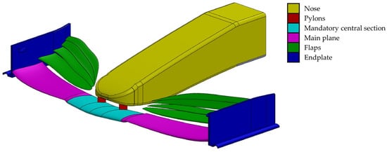
Figure 1. Parts of the front wing prior to the change in the technical regulations.

Compared to the old design, the new front wing design that the new technical regulations created has a more straightforward shape but with excellent aerodynamic efficiency despite reducing the load generated by this device. This new design has a longer nose in which the flaps are mounted directly; these curve to join in a single piece that makes up the endplate; this element has a shape similar to a shark’s fin; in this way, the mandatory central section and the pylons were eliminated (Figure 2) [15,18,19].

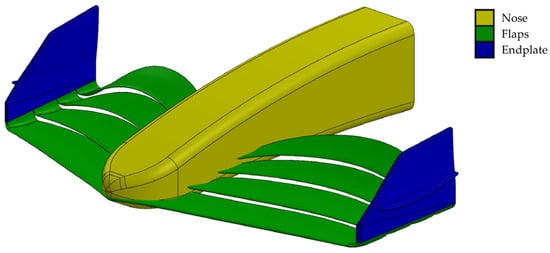
Figure 2. Parts of the current design of the front wing.

To determine the endplate’s importance in the front wing’s aerodynamic performance, a numerical analysis was conducted through computational simulations using the finite volume method [20,21]. To carry out this numerical analysis, the work team began by defining the study cases that will be addressed in this work. The authors decided to focus on two operating conditions; the first is the analysis of the front wing under conditions of travel along a straight line at high speed, and the second is the passage through a medium-speed curve.

For each operation case, two simulations will be carried out. The first uses a complete front wing model (without damage) that includes the suspension and front wheels of the car. In contrast, the second uses an identical model in which the endplates have been removed (pretending to be damaged) (Figure 3). The work team decided to focus on these two case studies because in slow curves, the speed is so low that the vehicle’s aerodynamics are left aside, and, on the contrary, fast curves tend to be so shallow that they can be considered practically straight.

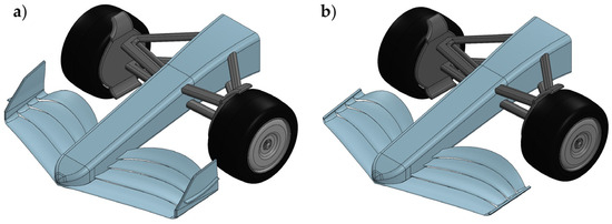
Figure 3. (a) Complete front wing model; (b) front wing model without endplates.

2.2. Governing Equations

CFD was used to perform this series of steady-state numerical analyses; the turbulence model used was the k-ω SST model [8,22,23]. The Reynolds number is a dimensionless number that describes a fluid’s behavior. Depending on its value, it is possible to determine whether a flow is laminar or turbulent; since the Reynolds number for the straight-line simulation is Re = 2.88 × 10⁶ and for the curve simulation it is Re = 1.62 × 10⁶, we can thus obtain both the graphic results and numbers to understand the effects caused by this change in the geometry of the front wing. The reason for choosing to carry out the simulations using this turbulence model is due to the superiority in saving computational resources without sacrificing the quality of the results in the numerical analyses [24,25]; in addition, this turbulence model is widely used in the automotive sector due to its extensive advantages over other models [9,22,26].

To describe and understand the k-ω SST turbulence model, it is necessary to review the mathematical formulations governing it. Among these governing equations are the conservation equations of mass and momentum, as shown below [27]:

$${\displaystyle \frac{\partial u_i}{\partial x_i}}=0$$

(1)

$$\rho u_j{\displaystyle \frac{\partial u_i}{\partial x_j}}=-{\displaystyle \frac{\partial p}{\partial x_i}}+{\displaystyle \frac{\partial }{\partial x_j}}\left(2v{S}_{ij}-\rho \overline{u_i^{\prime }{u}_j^{\prime }}\right)$$

(2)

2.3. k-ω SST Turbulence Model

This turbulence model was developed by F. R. Menter in the early 1990s and was named k-ω Shear Stress Transport since in general terms, it is considered an advance on the standard k-ω model established by D. C. Wilcox; it uses the k-ε model for the free flow region due to its robustness and to be able to perceive the effects generated near the wall due to its reliable precision [28,29].

The transport equations for the k-ω SST model are presented below [30,31]:

$$U_j{\displaystyle \frac{\partial k}{\partial x_j}}=P_k-{\beta }^{*}k\omega +{\displaystyle \frac{\partial }{\partial x_j}} \left[\left(v+{\sigma }_k{v}_t\right){\displaystyle \frac{\partial k}{\partial x_j}}\right]$$

(3)

$$U_j{\displaystyle \frac{\partial \omega }{\partial x_j}}=\gamma S^2-{\beta \omega }^2+{\displaystyle \frac{\partial }{\partial x_j}} \left[\left(v+{\sigma }_{\omega }{v}_t\right){\displaystyle \frac{\partial \omega }{\partial x_j}}\right]+2\left(1-F_1\right){\sigma }_{\omega 2}{\displaystyle \frac{1}{\omega }}{\displaystyle \frac{\partial k}{\partial x_i}}{\displaystyle \frac{\partial \omega }{\partial x_i}}$$

(4)

The model constants are determined by the following equations:

$$\gamma =F_1{\gamma }_1+\left(1-F_1\right){\gamma }_2$$

(5)

$${\gamma }_1={\displaystyle \frac{{\beta }_1}{{\beta }^{*}}}-{\sigma }_{\omega 1}{\displaystyle \frac{k^2}{\sqrt{{\beta }^{*}}}}$$

(6)

$${\gamma }_2={\displaystyle \frac{{\beta }_2}{{\beta }^{*}}}-{\sigma }_{\omega 2}{\displaystyle \frac{k^2}{\sqrt{{\beta }^{*}}}}$$

(7)

The eddy viscosity v_t is defined by the equation below:

$$v_t={\displaystyle \frac{a_{1}k}{max\left(a_1\omega ,S{F}_2\right)}}$$

(8)

The blending functions F₁ and F₂ can be determined using the following equations:

$$F_1=\tanh \left\{{\left\{min\left[max\left({\displaystyle \frac{\sqrt{k}}{0.09\omega d}},{\displaystyle \frac{500v}{d^2\omega }}\right),{\displaystyle \frac{2k}{{CD}_{k\omega }{d}^2}}\right]\right\}}^4\right\}$$

(9)

$$F_2=\tanh \left[{\left\{max\left({\displaystyle \frac{2\sqrt{k}}{{\beta }^{*}\omega d}},{\displaystyle \frac{500v}{d^2\omega }}\right)\right\}}^2\right]$$

(10)

To obtain the cross-diffusion term CD_kω, the following equation is used:

$${CD}_{k\omega }=max\left({\displaystyle \frac{1}{\omega }}{\displaystyle \frac{\partial k}{\partial x_i}}{\displaystyle \frac{\partial \omega }{\partial x_i}},{10}^{-20}\right)$$

(11)

Aerodynamic coefficients are dimensionless variables that describe the behavior of a body moving through the air. These three coefficients are named after the aerodynamic forces that act on the body, which are C_Df (Downforce), C_D (Drag), and C_Y (Yaw moment) [32]:

$$C_{Df=}{\displaystyle \frac{Downforce}{\frac{1}{2}\rho V^{2}A}}$$

(12)

$$C_{D=}{\displaystyle \frac{Drag}{\frac{1}{2}\rho V^{2}A}}$$

(13)

$$C_{Y=}{\displaystyle \frac{Yaw}{\frac{1}{2}\rho V^{2}A}}$$

(14)

3. Numerical Analyses

3.1. Generalities

The model used in this research work is based on a front wing model previously designed by the work team [32], and which is adequate for the requirements dictated by the current FIA technical regulations for the Formula One championship [19]. The model is composed of the nose of the car as well as the flaps and the endplates which make up the front wing. However, with the intention of conducting a more comprehensive study and understanding the aerodynamic effects that are generated by the rotation of the wheels [33,34,35], the work team decided to integrate the suspension and the wheels of the vehicle.

A double wishbone type suspension was integrated that includes a pushrod; in addition to wheels with a diameter of 725 mm and a thickness of 360 mm, whose outer faces are at 2000 mm from each other, the distance between the axis of the front wheels and the frontmost part of the model is 1350 mm. The front wing also has a wingspan of 2000 mm, the nose is 2000 mm long, and the highest part of it is 690 mm from the ground, while the total height of the model is 745 mm due to the over-wheel winglets that can be seen above the wheels (Figure 4).

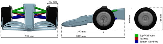
Figure 4. Model dimensions.

All the simulations in this research were carried out using the Fluent tool, which is part of the ANSYS^® Workbench 2021 R2 software; this, in turn, was chosen to use a coupled solver based on the SIMPLE algorithm since it allows for improving the consumption of the capacity of computational resources [7,36]. The Fluent tool is made up of modules with which the user interacts to be able to define the conditions of the analysis, carry out the solution, and obtain the results.

3.2. Straight-Line Simulation

This section describes the process of defining the conditions under which the simulations of maximum speed in a straight line were carried out for the model with endplates and the model without them. The speed at which the airflow will be found for this simulation is 320 km/h for both the model with and without endplates.

3.2.1. Geometry Module

In this first module, the domain is defined; to accomplish this, the first step is to import the geometries from an external CAD design software (SolidWorks 2024) where the two front wing models were previously designed. Subsequently, it is necessary to define the dimensions of the control volume.

The control volume is the region around the model where we want to know the effects generated by the airflow that interacts with the solid. To define the dimensions of the control volume, the investigation performed by Jacuzzi et al. [37] and by Ljungskog et al. [38] was considered, where the sizing of the control volume is not directly related to the dimensions of the body under study; however, due to the large size they propose for the control volume, they manage to obtain a blockage ratio with a low value. Differently, Fu et al. [30], Zhang et al. [31], Simmonds et al. [39], and Chode et al. [40] present a way to define the size of the control volume based on the dimensions of the body being studied, such as length (L), width (W), and height (H), in order to use them as basic sizing units; in this way, they manage to obtain a control volume proportional to the element under study, achieving an acceptable blockage ratio without compromising the analyses using a domain with excessive size. For the simulations presented in this work, a control volume of 4 W wide, 6 H high, 1 L upstream, and 6 L downstream is defined, giving a total of 8 L long (Figure 5); with these dimensions, it is possible to obtain for both models with and without endplates a blocking ratio of 3.237%, which is considered adequate to obtain reliable data [36,41].

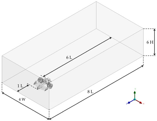
Figure 5. Control volume with front wing for straight-line simulation.

3.2.2. Mesh Module

The following module enables the discretization of complete systems. To optimize the process of obtaining results, a mesh independence study was undertaken. This efficient approach ensures that accurate results can be obtained without compromising computational consumption, using an appropriate mesh that does not have an excessive number of elements [42].

To carry out this independence test, it is necessary to present a series of meshes for both models, each with more elements and nodes. Subsequently, an analysis is carried out with each domain already discretized using the same boundary conditions for each simulation. Finally, when obtaining the results, it is necessary to compare them with each other to find the mesh that delivers accurate results without excessively consuming the computing equipment’s resources.

For all the simulations developed in this research, a semi-controlled method was used with high-order elements and a refinement of the elements’ size on the model’s surface as well as inflation layers. Five meshes were developed per model, ranging from Coarse to Very Fine with different refinement qualities: the first of them has 300 mm elements in the outermost zone and 20 mm on the surface of the front wing; the second has 250 mm elements in the outermost zone and 16 mm on the surface of the front wing; the third presents 200 mm elements in the outermost zone and 12 mm on the surface of the front wing; the fourth presents 150 mm elements in the outermost zone and 8 mm on the surface of the front wing; and the final mesh presents 100 mm elements in the outermost zone and 4 mm on the front wing surface (Figure 6). In addition, 30 inflation layers were integrated into this mesh with a growth rate of 1.2.

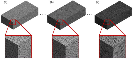
Figure 6. Discretized domains presented for the mesh independence test: (a) Coarse mesh; (b) Mid-Fine mesh; (c) Very Fine mesh.

With the discretized meshes, the test continued by performing a computational simulation to find the values of the aerodynamic coefficients C_Df and C_D to compare them. These results for the model with endplates are presented in Table 1, and the results for the model without endplates are presented in Table 2.

Table 1. Results of the independence test for the model with endplates in straight-line simulation.

Mesh	Nodes	Elements	Y+	CDf	CD
Coarse	9,753,018	26,385,356	≈25.07	1.83998	0.52864
Medium	15,023,893	47,932,793	≈10.75	1.83232	0.52121
Mid-Fine	20,400,768	69,487,821	≈4.89	1.82796	0.51635
Fine	25,130,644	90,042,577	≈1.85	1.82553	0.51408
Very Fine	31,058,495	114,891,067	≈0.98	1.82522	0.51373

Table 2. Results of the independence test for the model without endplates in straight-line simulation.

Mesh	Nodes	Elements	Y+	CDf	CD
Coarse	9,977,923	26,951,057	≈26.32	1.79191	0.56634
Medium	15,370,356	48,960,475	≈10.88	1.78177	0.55660
Mid-Fine	20,871,291	70,977,640	≈5.12	1.77728	0.55171
Fine	25,710,154	91,973,086	≈1.93	1.77555	0.55018
Very Fine	31,774,703	117,354,332	≈1.05	1.77541	0.55011

When observing the data obtained, both independence tests present similar behaviors in how the aerodynamic coefficients vary. Focusing on the results of the test of the model with endplates and taking the Very Fine mesh as a reference and comparing it with the Coarse mesh, there is a difference in the C_Df of 0.8086% and 2.8945% in the C_D; this difference reduces as a discretized mesh with a higher refinement like that of the Fine mesh where the difference with respect to the Very Fine mesh is only 0.0169% in the C_Df and 0.0681% in C_D. This same trend, in which the differences of the values obtained from the aerodynamic coefficients tend to be reduced, is repeated for the test of the model without endplates. The Fine mesh was chosen to use for both study cases because the work team considers the resolution in the results obtained to be acceptable. Using the Very Fine mesh would require a high consumption of the computational resources that the work team has access to. Analyzing the mesh metrics for both domains, it was determined that the quality of the meshes is adequate to perform simulations with accurate results. The mesh for the model with endplates has an orthogonal quality between 0.85 and 0.96, a skewness between 0.22 and 0.41, and a Y+ ≈ 1.85; on the other hand, the mesh for the model without endplates has an orthogonal quality between 0.83 and 0.97, a skewness between 0.22 and 0.43, and a Y+ ≈ 1.93; all these values are considered suitable to carry out the simulations [8,43].

3.2.3. Setup Module

Once the meshes have been defined for the two study cases, it is necessary to define the boundary conditions for the simulation (Figure 7) [8,13]. As mentioned above, the displacement of the front wing in a straight line was simulated at a speed of 320 km/h using the k-ω SST model with a turbulence intensity of 5%. Table 3 presents a description of the boundary conditions for the domain surfaces.

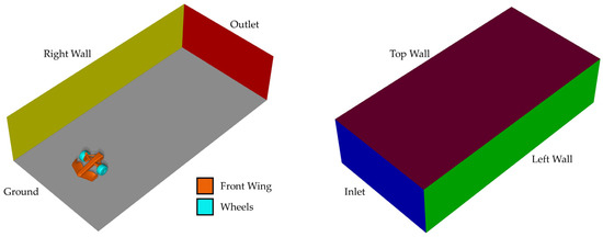
Figure 7. Boundary conditions for straight-line simulations.

Table 3. Summary of the boundary conditions used in straight-line simulations.

Surface	Boundary Conditions	Details
Front Wing	No-slip Stationary wall	No-slip. No movement.
Wheels	No-slip Rotational wall	No-slip. Angular velocity of 253.9682 rad/s.
Inlet	Velocity inlet	320 km/h airflow speed. Airflow normal to the surface.
	Turbulence Intensity	5% for all simulations.
Outlet	Outlet pressure	Allows recirculation.
Left Wall	Outlet pressure	Allows recirculation.
Right Wall	Outlet pressure	Allows recirculation.
Top Wall	Outlet pressure	Allows recirculation.
Ground	No-slip Moving wall	No-slip. Translation speed of 320 km/h in the direction of the airflow.

The simulations in this research were based on the physical properties of the fluid, which were set to mirror those of air at sea level according to the Standard International Atmosphere. This choice, where the density = 1.225 kg/m³, atmospheric pressure = 101.325 KPa, dynamic viscosity = 1.8 × 10^–5 Pa·s, and temperature = 288.15 K, was a crucial foundation for our work. Additionally, the dimensionless constants used by the turbulence model were defined as follows: σK1= 1.176, σω1 = 2.0, σK2 = 1.0, σω2 = 1.168, α1= 0.31, βi1 = 0.075, βi2 = 0.0828 [9,44].

To ensure that the results converge on a precise solution, it was decided that the number of iterations that the software would perform would be independent for each simulation, focusing on achieving homogeneity in the residuals [8].

3.3. Medium-Speed Curve Simulation

Like the previous section, this describes the conditions under which the simulation of passing through a medium-speed curve that turns to the right was carried out [7,12,13]. To achieve this situation, an airflow angle of 20° was determined based on the axis of symmetry and a speed of 180 km/h. The model used was identical to the one used in the straight-line simulation, with the difference that the suspension and wheel angles were adjusted so that the front wing’s resulting trajectory coincided with the airflow angle (Figure 8).

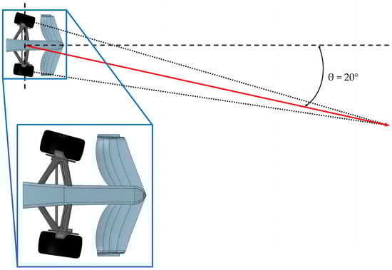
Figure 8. Front wing model for the medium-speed curve simulation.

3.3.1. Geometry Module

After adjusting the suspension and wheels to the front wing, the geometry was imported into the ANSYS^® Workbench software to define the characteristics of the control volume. The overall dimensions of the control volume for the curve simulations are the same as those used for the straight-line simulation; however, to achieve the effect in which the airflow describes a curved path, it is necessary to make an adjustment to the surfaces of the two lateral faces of the control volume and divide them to thus have four faces [12]. This division was performed by drawing a line perpendicular to the symmetry axis of the car at 2 L from the front face of the control volume just at the rear end of the front wing model (Figure 9).

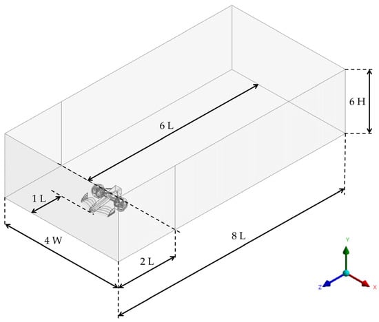
Figure 9. Control volume with front wing for medium-speed curve simulation.

3.3.2. Mesh Module

A mesh independence study was also performed for this second series of simulations to find the most appropriate mesh [42]. Because the front wing model for the curve only presents differences in the position of the wheels and suspension compared to the model for the straight line, and since the control volume has the same size in both cases, it was decided to develop five meshes by returning to identify the same qualities of refinement as in the previous test. A semi-controlled method with high-order elements was used to generate these meshes; 30 inflation layers were integrated into this mesh with a growth rate of 1.2.

After generating the five meshes for the model with endplates and the model without endplates, a simulation was performed to find the values of the aerodynamic coefficients C_Df and C_D. These results for the model with endplates are presented in Table 4, and the results for the model without endplates are presented in Table 5.

Table 4. Results of the independence test for the model with endplates in medium-speed curve simulation.

Mesh	Nodes	Elements	Y+	CDf	CD
Coarse	9,761,892	26,396,027	≈25.02	1.48942	0.37425
Medium	15,027,154	47,943,586	≈10.03	1.47944	0.36653
Mid-Fine	20,405,851	69,498,722	≈4.68	1.47297	0.36284
Fine	25,134,209	90,055,429	≈1.76	1.46858	0.36167
Very Fine	31,063,557	114,905,047	≈0.88	1.46803	0.36121

Table 5. Results of the independence test for the model without endplates in medium-speed curve simulation.

Mesh	Nodes	Elements	Y+	CDf	CD
Coarse	9,985,740	26,967,488	≈29.38	1.23141	0.35123
Medium	15,378,158	48,976,504	≈12.17	1.21982	0.34417
Mid-Fine	20,879,506	70,993,298	≈5.49	1.21249	0.33985
Fine	25,718,472	91,990,356	≈1.95	1.20891	0.33840
Very Fine	31,783,664	117,371,285	≈1.13	1.20845	0.33797

As with the independence tests for the straight-line models, the results for the meshes generated for the curve-passing models present the same behavior where the Fine mesh reaches a precision considered adequate to perform the simulations for the model with endplates and the model without endplates. Analyzing the mesh metrics for both domains, it was determined that the quality of the meshes is adequate to perform simulations with accurate results. The mesh for the model with endplates has an orthogonal quality between 0.83 and 0.97, a skewness between 0.23 and 0.43, and a Y+ ≈ 1.76; on the other hand, the mesh for the model without endplates has an orthogonal quality between 0.84 and 0.95, a skewness between 0.21 and 0.40, and a Y+ ≈ 1.95; all these values are considered suitable to carry out the simulations [8,43].

3.3.3. Setup Module

Since the meshes were defined for the two study cases, it is necessary to define the boundary conditions for the simulation. In this second case study, the displacement of the front wing was simulated through a medium-speed curve that turns to the right at a speed of 180 km/h with an angle of 20° using the k-ω SST model with a turbulence intensity of 5%. An adjustment was made to the lateral surfaces of the control volume in the geometry module. To ensure that the airflow path describes a curve, it is necessary to integrate an arrangement of inlets and outlets [12] (Figure 10).

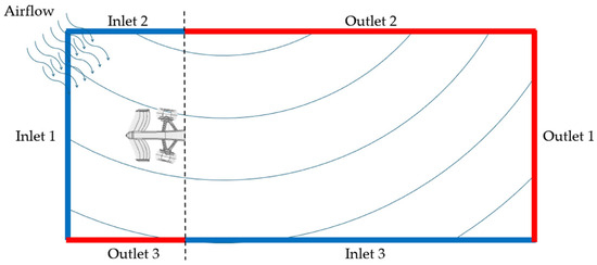
Figure 10. Arrangement for cornering simulation.

In addition to the arrangement of inputs and outputs on the outer lateral faces of the control volume, it is necessary to consider the rotation since the wheels do not follow the same trajectory; the speed is not the same in this case, where the curve is towards the left. Indeed, the wheel inside the curve has a lower speed than the outside wheel. The boundary conditions for these simulations are presented in Table 6.

Table 6. Summary of the boundary conditions used in medium-speed curve simulations.

Surface	Boundary Conditions	Details
Front Wing	No-slip Stationary wall	No-slip. No movement.
Right Wheel	No-slip Rotational wall	No-slip. Angular velocity of 139.2857 rad/s.
Left Wheel	No-slip Rotational wall	No-slip. Angular velocity of 146.4285 rad/s.
Inlet 1	Velocity inlet Turbulence Intensity	180 km/h airflow speed. Airflow defined through its three-dimensional components. 5% for all simulations.
Inlet 2	Velocity inlet Turbulence Intensity	180 km/h airflow speed. Airflow defined through its three-dimensional components. 5% for all simulations.
Inlet 3	Velocity inlet Turbulence Intensity	180 km/h airflow speed. Airflow defined through its three-dimensional components. 5% for all simulations.
Outlet 1	Outlet pressure	Allows recirculation.
Outlet 2	Outlet pressure	Allows recirculation.
Outlet 3	Outlet pressure	Allows recirculation.
Ground	No-slip Moving wall	No-slip. Translation speed of 180 km/h in the direction of the airflow.

The same physical properties of the fluid and dimensional constants for the turbulence model were defined as in the straight-line simulations [16,35]. Likewise, the number of iterations was independent for each simulation to converge on a precise solution seeking homogeneity in the residuals [10].

4. Results and Discussion

4.1. Straight-Line Simulation

Below are some of the graphical and numerical results obtained from the first series of straight-line simulations. Figure 11 compares the Pressure coefficients (Cp) present on the surfaces of the front wing and the suspension for both models analyzed.

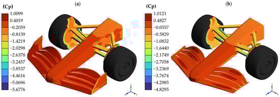
Figure 11. Cp present on the surfaces in straight-line simulation: (a) model with endplates; (b) model without endplates.

The highest Cp value in the model with endplates is 1.0099, which is slightly lower than the highest Cp on the surface of the model without endplates, which is 1.0121. Despite this, these high-pressure zones are present on most of the upper surface of the fins and in the internal front area of the endplates.

If the front wing is observed from a lower view, the Cp distribution in this region can be appreciated. Figure 12 shows how the model with endplates presents lower pressures than the one without. Furthermore, in the model with endplates, there is a significant positive pressure zone located in the majority of the lower area of the car’s nose.

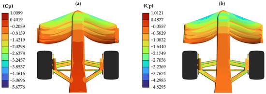
Figure 12. Cp present on the surfaces in straight-line simulation from a bottom view: (a) model with endplates; (b) model without endplates.

Figure 13 shows the Cp results on the model’s wheels. Because the wheels are rotating, it was decided to present these results independently of the pressures exerted on the surface of the front wing to understand the performance of these elements in isolation.

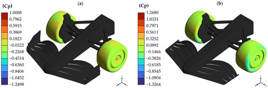
Figure 13. Cp present on the wheels in straight-line simulation: (a) model with endplates; (b) model without endplates.

After analyzing the previous figure, it is possible to perceive how the model without endplates presents a more significant number of low-pressure areas on the outer lateral face of the wheels, in particular just behind the end where the flaps join to give way to the endplate; this low-pressure zone is due to the lack of an endplate that prevents the generation of vortices that affect the wheel and is accompanied by an effect in which the entire wheel suffers from both higher and lower pressures compared to the wheels of the model with endplates where the pressure distribution presents greater homogeneity on the external lateral face of the wheels.

Figure 14 depicts the Cp distribution in the air around the front wing on the XY plane 850 mm in front of the axis of the front wheels, just above the region where the flaps and endplates are located. It is clear that the endplates play a crucial role in creating a high-pressure zone above the flaps and the nose of the car, effectively isolating it from the area below the front wing. This high-pressure zone is larger when equipped with endplates. Both models reach almost identical highest pressures, but the model with endplates demonstrates superior efficiency in isolating the area below the front wing, reaching lower pressures than the model without endplates. This highlights the importance of endplates in creating a high-pressure zone.

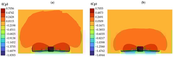
Figure 14. Cp present on the air around the front wing in straight-line simulation: (a) model with endplates; (b) model without endplates.

The software also allows for obtaining numerical results to determine the aerodynamic forces acting on the models; Table 7 presents the results of the aerodynamic coefficients for the model with endplates, while Table 8 presents the same results for the model without endplates.

Table 7. Summary of aerodynamic coefficients for the model with endplates in straight-line simulation.

Element	CDf	CD	CY
Front Wing	−3.04048	−0.45304	−0.00556
Right Wheel	−0.07296	−0.50102	−0.17995
Left Wheel	−0.07105	−0.49773	−0.17257
Total Model	−1.82551	−0.51386	0.00862

In these results, the negative sign only indicates the direction that the force has according to the positive direction of the three-dimensional coordinates.

Table 8. Summary of aerodynamic coefficients for the model without endplates in straight-line simulation.

Element	CDf	CD	CY
Front Wing	−3.07373	−0.46290	−0.01564
Right Wheel	−0.04558	−0.57790	0.19485
Left Wheel	−0.04671	−0.57898	−0.20196
Total Model	−1.77591	−0.55030	−0.01712

In these results, the negative sign only indicates the direction that the force has according to the positive direction of the three-dimensional coordinates.

By analyzing the data obtained from the aerodynamic coefficients and comparing them with each other, it is possible to define the importance of the endplates in the aerodynamic efficiency of the front wing and the front wheels. If the model is analyzed thoroughly, a decrease in C_Df of 2.716%, an increase of 7.092% in C_D, and an increase of 96.332% in C_Y can be calculated when the front wing does not have endplates. If the results are analyzed individually for each element, it can be determined how they are affected when the model does not have endplates. Focusing only on the front wing, it was calculated that the endplates increased 2.055% of the total C_Df, the C_D increased by 1.008%, and the C_Y increased by 177%; the right wheel lost 37.521% of C_Df, but its C_D increased by 15.344%, and its C_Y by 8.279%. In comparison, the left wheel suffered a decrease of 34.259% in C_Df but an increase of 16.324% in C_D and an increase of 17.030% in C_Y. Figure 15 presents a series of graphs that compare the results of the aerodynamic coefficients obtained from the simulation of a straight line at maximum speed.

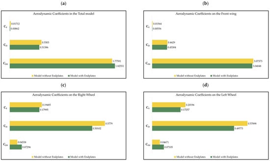
Figure 15. Comparison of the aerodynamic coefficients present on the different elements in the straight-line simulation: (a) total model; (b) front wing; (c) right wheel; (d) left wheel.

The data indicate that the aerodynamic coefficients generated by the front wing when it does not have endplates are affected, reducing the efficiency of this element; mainly, an increase in the C_Y is seen, which causes the car to generate lateral vibrations that make it unstable at maximum speed; however, it turns out that the wheels are the elements that are most affected. Figure 16 shows the eddy viscosity of both models; since there are no endplates at the ends of the flaps, there is greater dissipation in the flow over the wheels. Figure 17 and Figure 18 present the iso-surfaces of the Q-criterion (Q = 0.005) and vorticity to exemplify the turbulences generated in the straight-line simulation model with endplates and without endplates, respectively. The velocities reached by the airflow were plotted on these iso-surfaces.

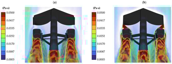
Figure 16. Eddy viscosity in straight-line simulation: (a) model with endplates; (b) model without endplates.

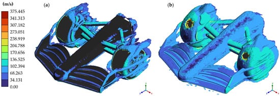
Figure 17. Iso-surfaces on model with endplates for straight-line simulation: (a) Q-criterion; (b) vorticity.

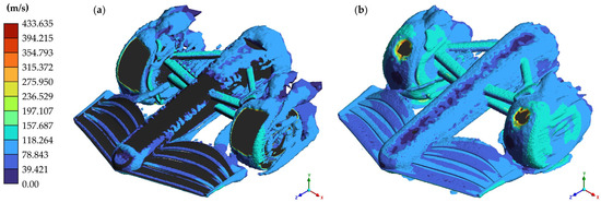
Figure 18. Iso-surfaces on model without endplates for straight-line simulation: (a) Q-criterion; (b) vorticity.

4.2. Medium-Speed Curve Simulation

Below are some of the graphical and numerical results obtained from the simulations of medium-speed curves. Figure 19 compares the Cp present on the front wing and suspension surfaces for both models analyzed.

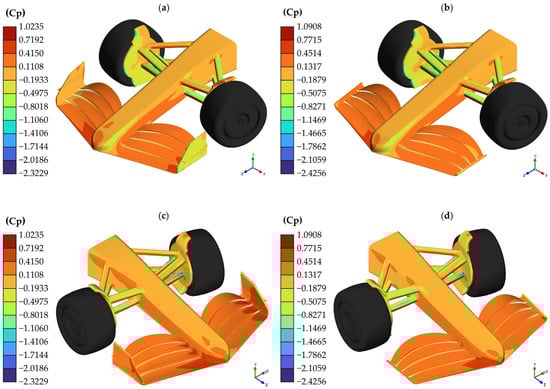
Figure 19. Cp present on the surfaces in medium-speed curve simulation: (a,c) model with endplates; (b,d) model without endplates.

When the two front wing models are observed from below, it can be seen how the Cp distribution in this region exhibits a similar behavior for both cases; the lowest pressures occur in the lower area of the most frontal flaps on the right side, which are the first to encounter the airflow. On the contrary, there is an area of positive pressure in the lower area of the rearmost flaps on the left side, as seen in Figure 20. It can also be seen how the model without endplates presents an area of positive pressure on the lower area of the nose of the car that is greater than that presented by the model that does have these elements.

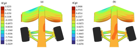
Figure 20. Cp present on the surfaces in medium-speed curve simulation from a bottom view: (a) model with endplates; (b) model without endplates.

In the same way as with the results of the previous simulation, it was decided to present the results of the pressure coefficients on the wheels in isolation since they have different magnitudes in the pressures reached than the surface of the front wing. Figure 21 presents the Cp distribution on the wheels from different positions.

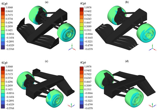
Figure 21. Cp present on the wheels in medium-speed curve simulation: (a,c) model with endplates; (b,d) model without endplates.

After analyzing the Cp distribution on the wheels, it is possible to observe how both models exhibit very similar behaviors where the lateral faces of the wheels present lower pressures than those presented on the tread. Although the behavior is similar, the Cp on the wheels without endplates reaches higher levels. The highest recorded Cp went from 1.0048 to 1.0978 when there were no endplates, while the minimum recorded pressure went from −0.5768 to −0.6378.

For the Cp distribution of air around the front wing, Figure 22 presents these pressure coefficients on an XY plane 850 mm in front of the axis of the front wheels.

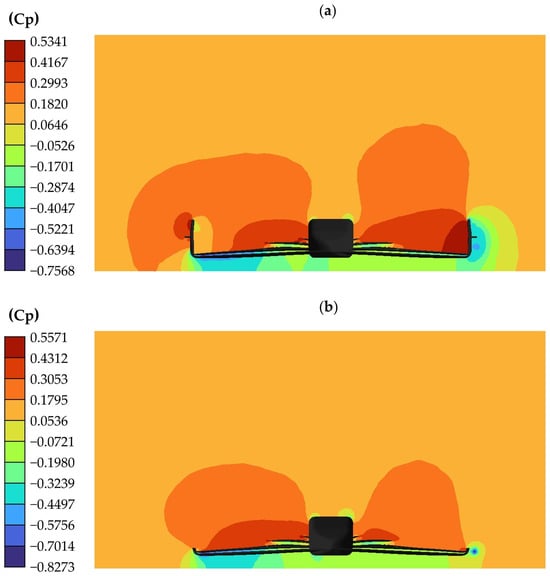
Figure 22. Cp present on the air around the front wing in medium-speed curve simulation: (a) model with endplates; (b) model without endplates.

When comparing the Cp distribution of both models with each other, it is possible to highlight how the pressures below the front wing behave in a pretty similar way since the lowest pressure area is located below the right flaps; despite this similarity, the Cp above and on the sides of the front wing behaves in different ways. The model with endplates has high-pressure areas on the right side of each endplate and a low-pressure region on the left side. This pressure difference generates a greater lateral force than the model that does not have endplates. Data for the aerodynamic coefficients for the model with endplates are presented in Table 9, while the results for the model without endplates are presented in Table 10.

Table 9. Summary of aerodynamic coefficients for the model with endplates in medium-speed curve simulation.

Element	CDf	CD	CY
Front Wing	−2.14751	−0.24532	0.43623
Right Wheel	−0.51008	−0.50094	0.33449
Left Wheel	−0.32285	−0.38213	0.18847
Total Model	−1.47032	−0.36295	0.64698

In these results, the negative sign only indicates the direction that the force has according to the positive direction of the three-dimensional coordinates.

Table 10. Summary of aerodynamic coefficients for the model without endplates in medium-speed curve simulation.

Element	CDf	CD	CY
Front Wing	−1.78301	−0.22854	0.28161
Right Wheel	−0.50093	−0.48658	0.32534
Left Wheel	−0.27912	−0.35755	0.18175
Total Model	−1.20996	−0.33924	0.50888

In these results, the negative sign only indicates the direction that the force has according to the positive direction of the three-dimensional coordinates.

To determine the aerodynamic efficiency of the endplates and their importance in the operation of the front wing when taking a medium-speed curve, it is necessary to compare the results obtained for each model. For this, it is necessary to determine if the aerodynamic coefficients tend to increase or decrease. Comparing the results for the total model, it is determined that when there are no endplates, there is a total reduction of 17.707% in C_Df, 6.532% in C_D, and 22.200% in C_Y. When the elements are compared independently, it is determined that the loss of aerodynamic forces occurs in all the elements of the model when there are no endplates; the front wing loses 19.559% of C_Df, 9.743% of C_D, and 36.255% of C_Y; the right wheel loses 1.792% of C_Df, 2.867% of C_D, and 2.736% of C_Y; and finally the left wheel has a decrease of 13.545% in C_Df, 6.431% in C_D, and 3.564% in C_Y. Figure 23 presents a series of graphs that compare the results of the aerodynamic forces obtained from the simulation of passing through a medium-speed corner.

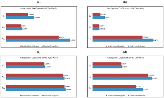
Figure 23. Comparison of the aerodynamic coefficients present on the different elements in medium-speed curve simulation: (a) total model; (b) front wing; (c) right wheel; (d) left wheel.

After analyzing the data on the aerodynamic coefficients, it is essential to highlight the differences in the model’s behavior when it has or does not have endplates when cornering. The decrease in C_Y presented by the model without endplates is advantageous since this force causes the vehicle to suffer from lateral forces that push it to lose control and shoot out of the curve. Figure 24 shows the eddy viscosity for both models. Unlike in the straight-line simulation, the endplates generate more outstanding dissipation in the flow when cornering. Figure 25 and Figure 26 present the iso-surfaces of the Q-criterion (Q = 0.005) and vorticity to exemplify the turbulences generated in the model with and without endplates, respectively. The velocities reached by the airflow were plotted on these iso-surfaces.

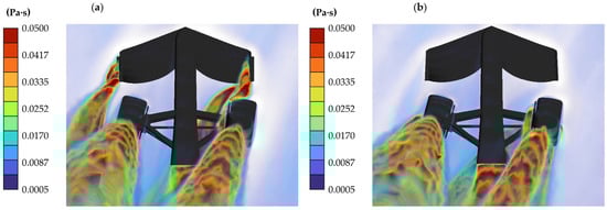
Figure 24. Eddy viscosity in medium-speed curve simulation: (a) model with endplates; (b) model without endplates.

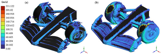
Figure 25. Iso-surfaces on model with endplates for medium-speed curve simulation: (a) Q-criterion; (b) vorticity.

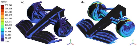
Figure 26. Iso-surfaces on model without endplates for medium-speed curve simulation: (a) Q-criterion; (b) vorticity.

Although the analysis’s numerical results have yet to be experimentally corroborated for this research work, it is essential to clarify that the methodology used has been proven in various investigations, resulting in a margin of error ranging from 0.5 to 3.25% in the work conducted by Laguna et al. [32] for research focused on Formula One competition vehicles, as well as comparisons made between the numerical and experimental methods in research, such as those carried out by Roberts et al. [7], Patel et al. [13], Desai et al. [33], and Ljungskog [37]. Since the methodology used in this work has been ratified by the research and work on which it has been based, it can be determined that the results are valid.

5. Conclusions

After analyzing the results obtained from the simulations, a conclusion was reached about the importance of the endplates in the efficiency of the front wing. In the case of simulations in a straight line at maximum speed, the Downforce is little affected since it only decreases by 2.716%, which does not represent an impact on performance. However, it is notable how the endplates fulfill the task of reducing the generation of vortices at the ends of the front wing flaps; after viewing the graphic results where the vortices generated by the two models during these simulations are presented, it can be seen how the front wheels turn out to be affected due to this phenomenon. These vortices interfere with the airflow that reaches the wheels, causing the wheels to suffer an increase in the resulting Yaw of 96.332%, which generates lateral forces that make the car somewhat unstable and, at the same time, produce an increase in the Drag generated by the wheels of 7.092% which in turn can compromise the aerodynamics of the other elements that make up the vehicle. With this evidence, it is determined that the loss of total Downforce turns out to be insignificant. However, the increase in Drag and Yaw generates unwanted effects that complicate the front wheels’ performance and the vehicle’s stability when reaching maximum speeds on a straight line.

Moving on to the simulation of passing through a medium-speed curve, it can be seen how the total aerodynamic forces are affected differently. In the case of the Downforce, this decreases by 17.707% when there are no endplates; the Drag decreases by 6.532% and the Yaw decreases by 22.200%. It is notable how the endplates play a more important role when taking a curve than when driving in a straight line; even so, it should be highlighted how the endplates present the generation of vortices in this case since they have a larger contact surface in the airflow. This situation causes both Drag and Yaw to suffer a decrease, which is beneficial in the vehicle’s performance since there is less opposition to the passage through the airflow and less generation of lateral forces that cause instability and loss of grip. Although this behavior has an advantage over the model with endplates, the Downforce is seriously affected, producing a loss of grip and consequently forcing the driver to reduce speed in curves to avoid losing control of the car.

With the information obtained, it can be concluded that the importance of endplates on the front wing of Formula One cars is of great relevance; when driving at maximum speeds, it is responsible for reducing the vorticity present at the ends of the flaps, which helps to maintain stability and also better isolates the areas of high and low air pressure around the wing, improving Downforce and reducing Drag; when taking a medium-speed curve, their primary function lies in the generation of Downforce since the results indicate that they negatively cause vortices that increase both Drag and Yaw. From an aerodynamic point of view, the loss of the endplates causes a considerable reduction in the efficiency of the front wing, which is why a pit stop to change this element would be necessary. This loss of efficiency not only affects the car’s performance but also the driver’s ability to control the car. However, other variables that intervene when this situation arises, such as the time lost when making a pit stop and the circuits’ different configurations, must be considered. In a circuit where the straights are predominant and there are few curves, the loss of efficiency would be less critical, which could mean that maintaining a front wing with reduced performance does not generate a notable disadvantage compared to the other cars. On the contrary, in a circuit where curves predominate, the loss of efficiency demands that the element be changed.

Furthermore, it is equally necessary to consider the moment of the race in which the loss of endplates occurs. If it occurs at the beginning, it would be prudent to make the change as soon as possible to avoid any potential performance issues. However, this decision could be more harmful than beneficial if it occurs at an advanced point, as the time lost in the pit stop could significantly affect the car’s overall race performance. Therefore, it is important to weigh the potential benefits of a repaired front wing against the potential time lost in the pit stop before making a decision.

This research team determines that if damage occurs in the first laps of the race, making a pit stop for repairs would be the appropriate decision; however, changing the front wing when stopping in the pits for a tire change could be another good way to return the car to top condition without consuming more time by making a stop just to repair the wing.

References

- Næss, H.E. A History of Organizational Change: The Case of Fédération Internationale de l’Automobile (FIA), 1946–2020, 1st ed.; Palgrave Macmillan: Cham, Switzerland, 2020; pp. 27–193. [Google Scholar]
- Hutton, R. Fédération Internationale de l’Automobile Centenary; Fédération Internationale de l’Automobile: Paris, France, 2004; pp. 113–161. [Google Scholar]
- Katz, J. Aerodynamics in motorsports. Proc. Inst. Mech. Eng. Part P J. Sports Eng. Technol. 2019, 235, 324–338. [Google Scholar] [CrossRef]
- Dominy, R.G. Aerodynamics of Grand Prix cars. Proc. IMechE Part D J. Automob. Eng. 1992, 206, 267–274. [Google Scholar] [CrossRef]
- Agathangelou, B.; Gascoyne, M. Aerodynamic Design Considerations of a Formula 1 Racing Car; SAE Technical Paper Series; SAE International: Warrendale, PA, USA, 1998. [Google Scholar]
- Mokhtar, W.A.; Lane, J. Racecar Front Wing Aerodynamics. SAE Int. J. Passeng. Cars—Mech. Syst. 2009, 1, 1392–1403. [Google Scholar] [CrossRef]
- Roberts, L.S.; Correia, J.; Finnis, M.V.; Knowles, K. Aerodynamic characteristic of a wing-and-flap configuration in ground effect and yaw. Proc. IMechE Part D J. Automob. Eng. 2016, 230, 841–854. [Google Scholar] [CrossRef]
- Castro, X.; Rana, Z.A. Aerodynamic and structural design of a 2022 Formula One front wing assembly. Fluids 2020, 5, 237–259. [Google Scholar] [CrossRef]
- Basso, M.; Cravero, C.; Marsano, D. Aerodynamic Effect of the Gurney Flap on the Front Wing of a F1 Car and Flow Interactions with Car Components. Energies 2021, 14, 2059. [Google Scholar] [CrossRef]
- Gere-Gurky, R.; Adhitya, M. Front Wing Aerodynamic Analysis of formula 1 Cars in 2018 and 2019 with Computational Fluid Dynamics (CFD). AIP Conf. Proc. 2024, 2710, 030006. [Google Scholar]
- Petrone, G.; Hill, C.; Biancolini, M. Track by Track Robust Optimization of a F1 Front Wing using Adjoint Solutions and Radical Basis Functions. In Proceedings of the 32nd AIAA Applied Aerodynamics Conference, Atlanta, GA, USA, 16–20 June 2014. [Google Scholar] [CrossRef]
- Keogh, J.; Barber, T.; Diasinos, S.; Doig, G. Techniques for Aerodynamic Analysis of Cornering Vehicles; SAE Technical Paper; SAE International: Warrendale, PA, USA, 2015. [Google Scholar]
- Patel, D.; Garmory, A.; Passmore, M. The Effect of Cornering on the Aerodynamics of a Multi-Element Wingin Ground Effect. Fluids 2021, 6, 3. [Google Scholar] [CrossRef]
- Ahlfeld, R.; Ciampoli, F.; Pietropaoli, M.; Pepper, N.; Montomoli, F. Data-driven uncertainty quantification for Formula 1: Diffuser, wing tip and front wing variations. Proc. Inst. Mech. Eng. Part D J. Automob. Eng. 2019, 233, 1495–1506. [Google Scholar] [CrossRef]
- Fédération Internationale de l’Automobile. 2022 Formula One Technical Regulations, 2022 ed.; Fédération Internationale de l’Automobile: Geneve, Switzerland, 2022; p. 13. [Google Scholar]
- Formula One TV Archive. Available online: https://f1tv.formula1.com/page/493/archive (accessed on 15 July 2024).
- Fédération Internationale de l’Automobile. 2021 Formula One Technical Regulations, 2021 ed.; Fédération Internationale de l’Automobile: Geneve, Switzerland, 2021; p. 10. [Google Scholar]
- Fédération Internationale de l’Automobile. 2023 Formula One Technical Regulations, 2023 ed.; Fédération Internationale de l’Automobile: Geneve, Switzerland, 2023; p. 7. [Google Scholar]
- Fédération Internationale de l’Automobile. 2024 Formula One Technical Regulations, 2024 ed.; Fédération Internationale de l’Automobile: Geneve, Switzerland, 2024; p. 6. [Google Scholar]
- Minguez, M.; Pasquetti, R.; Serre, E. High-order large-eddy simulation of flow over the “Ahmed body” car model. Phys. Fluids 2008, 20, 095101. [Google Scholar] [CrossRef]
- Guilmineau, E.; Wackers, J. CFD Simulation with Automatic Mesh Refinement for the Flow around Simplifies Car Models. SAE Int. J. Passeng. Cars—Mech. Syst. 2012, 5, 580–591. [Google Scholar] [CrossRef]
- Guerrero, A.; Castilla, R. Aerodynamic Study of the Wake Effects on a Formula 1 Car. Energies 2020, 13, 5183. [Google Scholar] [CrossRef]
- Aultman, M.; Wang, Z.; Auza-Gutierrez, R.; Duan, L. Evaluation of CFD methodologies for prediction of flows around simplifies and complex automotive models. Comput. Fluids 2022, 236, 105297. [Google Scholar] [CrossRef]
- Menter, F.R.; Kuntz, M.; Langtry, R. Ten years of industrial experience with the SST turbulence model. Turbul. Heat Mass Transf. 2003, 4, 625–632. [Google Scholar]
- Afshari, F.; Zavaragh, H.G.; Sahin, B.; Grifoni, R.C.; Corvaro, F.; Marchetti, B.; Polonara, F. On numerical methods; optimization of CFD solution to evaluate fluid flow around a sample object at low Re numbers. Math. Comput. Simul. 2018, 152, 51–68. [Google Scholar] [CrossRef]
- Ehirim, O.H.; Knowles, L.; Saddington, A.J. A Review of Ground-Effect Diffuser Aerodynamics. J. Fluids Eng. 2019, 141, 020801. [Google Scholar] [CrossRef]
- Huang, H.; Sun, T.; Zhang, G.; Li, D.; Wei, H. Evaluation of a developed SST k-ω turbulence model for the prediction of turbulent slot jet impingement heat transfer. Int. J. Heat Mass Transf. 2019, 137, 700–712. [Google Scholar] [CrossRef]
- Menter, F.R. Two-Equation Eddy-Viscosity Turbulence Models for Engineering Applications. AIAA J. 1994, 32, 1598–1605. [Google Scholar] [CrossRef]
- Menter, F.R. Zonal Two Equation k-ω Turbulence Models for Aerodynamic Flows. In Proceedings of the AIAA 24th Fluid Dynamics Conference, Orlando, FL, USA, 6–9 July 1993. [Google Scholar]
- Fu, C.; Uddin, M.; Robinson, C.; Guzman, A.; Bailey, D. Turbulence Models and Model Closure Coefficients Sensitivity of NASCAR Racecar RANS CFD Aerodynamic Predictions. SAE Int. J. Passeng. Cars—Mech. Syst. 2017, 10, 330–344. [Google Scholar] [CrossRef]
- Zhang, C.; Bounds, C.P.; Foster, L.; Uddin, M. Turbulence Modeling Effects on the CFD Predictions of Flow over a Detailed Full-Scale Sedan Vehicle. Fluids 2019, 4, 148. [Google Scholar] [CrossRef]
- Laguna-Canales, A.S.; Urriolagoitia-Sosa, G.; Romero-Ángeles, B.; Martinez-Mondragon, M.; García-Laguna, M.A.; Correa-Corona, M.I.; Maya-Anaya, D.; Urriolagoitia-Calderón, G.M. Mechanical Design and Numerical Analysis of a New Front Wing for a Formula One Vehicle. Fluids 2023, 8, 210. [Google Scholar] [CrossRef]
- Desai, S.; Leylek, E.; Lo, C.-M.B.; Doddegowda, P.; Bychkovsky, A.; George, A.R. Experimental and CFD Comparative Case Studies of Aerodynaics of Race Car Wings, Underbodies with Wheels, and Motorcycle Flows; SAE Technical Paper Series; SAE International: Warrendale, PA, USA, 2008. [Google Scholar]
- Newbon, J.; Dominy, R.; Sims-Williams, D. CFD Investigation of the Effect of the Salient Flow Features in the Wake of a Generic Open-Wheel Race Car. SAE Int. J. Passeng. Cars—Mech. Syst. 2015, 8, 217–232. [Google Scholar] [CrossRef][Green Version]
- Diasinos, S.; Barber, T.; Doig, G. Numerical analysis of the effect of the change in the ride height on the aerodynamic front wing–wheel interactions of a racing car. Proc. Inst. Mech. Eng. Part D J. Automob. Eng. 2017, 231, 900–914. [Google Scholar] [CrossRef]
- Altinisik, A.; Kutukceken, E.; Umur, H. Experimental and Numerical Aerodynamic Analysis of a Passenger Car: Influence of the Blockage Ratio on Drag Coefficient. J. Fluids Eng. 2015, 137, 081104. [Google Scholar] [CrossRef]
- Jacuzzi, E.; Grandlund, K. Passive flow control for drag refuction in vehicle platoons. J. Wind Eng. Ind. Aerodyn. 2019, 189, 104–117. [Google Scholar] [CrossRef]
- Ljungskog, E.; Sebben, S.; Broniewicz, A. Inclusion of the physical wind tunnel in vehicle CFD simulations for improved prediction quality. J. Wind Eng. Ind. Aerodyn. 2020, 197, 104055. [Google Scholar] [CrossRef]
- Simmonds, N.; Pitman, J.; Tsoutsanis, P.; Jenkins, K.; Gaylard, A.; Jansen, W. Complete Body Aerodynamic Study of three Vehicles; SAE Technical Paper Series; SAE International: Warrendale, PA, USA, 2017. [Google Scholar]
- Chode, K.K.; Viswanathan, H.; Chow, K.; Reese, H. Investigating the aerodynamic drag and noise characteristics of a standard squareback vehicle with inclined side-view mirror configurations using a hybrid computational aeroacoustics (CAA) approach. Phys. Fluids 2023, 35, 075148. [Google Scholar] [CrossRef]
- Choi, C.K.; Kwon, D.K. Wind tunnel blockage effects on aerodynamic behavior of bluff body. Wind Struct. 1998, 1, 351–364. [Google Scholar] [CrossRef]
- Almohammadi, K.M.; Ingham, D.B.; Ma, L.; Pourkashan, M. Computational fluid dynamics (CFD) mesh independency techniques for a straight blade vertical axis wind turbine. Energy 2013, 58, 483–493. [Google Scholar] [CrossRef]
- Heide, J.; Karlsson, M.; Altimir, M. Numerical Analysis of Urea-SCR Sprays under Cross-Flow Conditions; SAE Technical Paper; SAE International: Warrendale, PA, USA, 2017. [Google Scholar]
- Soares, R.F.; de Souza, F.J. Influence of CFD Setup and Brief Analysis of Flow over a 3D Realistic Car Model; SAE Technical Paper Series; SAE International: Warrendale, PA, USA, 2015. [Google Scholar]
Disclaimer/Publisher’s Note: The statements, opinions and data contained in all publications are solely those of the individual author(s) and contributor(s) and not of MDPI and/or the editor(s). MDPI and/or the editor(s) disclaim responsibility for any injury to people or property resulting from any ideas, methods, instructions or products referred to in the content. |
© 2024 by the authors. Licensee MDPI, Basel, Switzerland. This article is an open access article distributed under the terms and conditions of the Creative Commons Attribution (CC BY) license (https://creativecommons.org/licenses/by/4.0/).