A Generalized Diffusion Equation: Solutions and Anomalous Diffusion

Abstract

We investigate the solutions of a generalized diffusion-like equation by considering a spatial and time fractional derivative and the presence of non-local terms, which can be related to reaction or adsorption–desorption processes. We use the Green function approach to obtain solutions and evaluate the spreading of the system to show a rich class of behaviors. We also connect the results obtained with the anomalous diffusion processes.

1. Introduction

Fractional calculus has quickly become a new efficient mathematical tool to analyze different properties of a given system and connect them with experimental results. A simple extension of the differential operators incorporating non-integer indexes has serious consequences, connecting the formalism with memory effects, long-range correlations, and many other features characterizing complex systems. In this manner, it has brought great insights into many fields of science [1,2,3,4,5,6]. One of them occurs for the diffusion processes, which have been found through fractional calculus a suitable approach to incorporate several effects which are not suitably described in terms of the classical integer order calculus. For instance, infiltration in porous building materials [7], the electrical response of electrolytic cells [6,8], amorphous semiconductors [9], and micellar solutions [10]. In these situations, there is a nonlinear time dependence exhibited by the mean-square displacement, which, in general, is characterized by $⟨{\left(x-⟨x⟩\right)}^2⟩\sim t^{\alpha }$, where $\alpha$ characterized the diffusion, e.g., $\alpha <1$, $\alpha =1$, and $\alpha >1$ correspond to the sub-, usual, and superdiffusion, respectively. This behavior of the mean square displacement and effects related, e.g., non-Markovian processes and fractal structure has motivated the analysis of different approaches, which extend the usual approach, such as fractional diffusion equations [11,12,13], master equation [14,15], generalized Langevin equations [16], and random walks [17]. One noticeable point regarding these extensions is that the behavior of the solutions is characterized by power laws and stretched exponential for fractional differential operators. In particular, the previous scenarios concerning the diffusion on fractals have indicated that the asymptotic form of the propagator, such as the Sierpinski gasket, is essentially in this form [11,18]. A similar situation is also found in fluid flow through porous media [19,20,21]. Other applications can be found in transport in the porous pellet [22], transport of chloride in concrete [23], and oxidation behaviors of needle-punched carbon/carbon composites [24].

Here, we consider the following extension of the diffusion equation:

$$\begin{array}{c}\hfill \frac{\partial }{\partial t}\rho (x,t)={}_0{\mathcal{D}}_t^{\gamma }{\int }_0^{\mu }d\overline{\mu }p\left(\overline{\mu }\right)D_x^{\overline{\mu },\eta }\rho (x,t)+{\int }_0^{t}d{t}^{\prime }\Lambda (t-t^{\prime })\rho (x,t^{\prime }),\end{array}$$

(1)

with $1\le \mu \le 2$, $-1<\eta$, $p\left(\overline{\mu }\right)$ is a distribution, ${}_0{\mathcal{D}}_t^{\gamma }\left(\cdots \right)$ is a fractional time operator, and $D_x^{\overline{\mu },\eta }(\cdots )$ is a spatial fractional operator [12,25]. The last term can be related to different processes, such as absorption and adsorption–desorption, depending on the choice of the kernel $\Lambda \left(t\right)$. It can also be related to reaction processes of the first order, i.e., irreversible reaction processes or reversible processes depending on the choice of $\Lambda \left(t\right)$. The fractional time operator ${}_0{\mathcal{D}}_t^{\gamma }(\cdots )$ is defined in terms of a generalized kernel ${\mathcal{K}}_{\gamma }\left(t\right)$ as follows:

$$\begin{array}{c}\hfill {}_0{\mathcal{D}}_t^{\gamma }\rho (x,t)=\frac{\partial }{\partial t}{\int }_0^{t}d{t}^{\prime }{\mathcal{K}}_{\gamma }(t-t^{\prime })\rho (x,t^{\prime }).\end{array}$$

(2)

Note that depending on the choice of ${\mathcal{K}}_{\gamma }\left(t\right)$ in the previous equation, we may connect it to different integrodifferential operators with singular or non-singular kernels. One of them is the Riemann–Liouville fractional operator, i.e., ${\mathcal{K}}_{\overline{\gamma }}\left(t\right)=t^{-\overline{\gamma }}/\Gamma \left(1-\overline{\gamma }\right)$ [26], which implies

$$\begin{array}{c}\hfill \frac{{\partial }^{\overline{\gamma }}}{\partial t^{\overline{\gamma }}}\rho (x,t)=\frac{1}{\Gamma \left(1-\overline{\gamma }\right)}\frac{\partial }{\partial t}{\int }_0^{t}d{t}^{\prime }\frac{1}{{(t-t^{\prime })}^{\overline{\gamma }}}\rho (x,t^{\prime }),\end{array}$$

(3)

another one is the Fabrizio–Caputo fractional operator, for ${\mathcal{K}}_{\overline{\gamma }}\left(t\right)$=${\mathcal{N}}_{\overline{\gamma }}{e}^{-\frac{\overline{\gamma }}{1-\overline{\gamma }}t}/(1-\overline{\gamma })$, i.e.,

$$\begin{array}{c}\hfill \frac{{\partial }^{\overline{\gamma }}}{\partial t^{\overline{\gamma }}}\rho (x,t)=\frac{{\mathcal{N}}_{\overline{\gamma }}}{1-\overline{\gamma }}\frac{\partial }{\partial t}{\int }_0^{t}d{t}^{\prime }{e}^{-\frac{\overline{\gamma }}{1-\overline{\gamma }}(t-t^{\prime })}\rho (x,t^{\prime }),\end{array}$$

(4)

or the Atangana–Baleanu fractional operator, for ${\mathcal{K}}_{\overline{\gamma }}\left(t\right)$=${\mathcal{N}}_{\overline{\gamma }}{E}_{\overline{\gamma }}\left(-\overline{\gamma }{t}^{\overline{\gamma }}/(1-\overline{\gamma })\right)/(1-\overline{\gamma })$, given by

$$\begin{array}{c}\hfill \frac{{\partial }^{\overline{\gamma }}}{\partial t^{\overline{\gamma }}}\rho (x,t)=\frac{{\mathcal{N}}_{\overline{\gamma }}}{1-\overline{\gamma }}\frac{\partial }{\partial t}{\int }_0^{t}d{t}^{\prime }{E}_{\overline{\gamma }}\left(-\frac{\overline{\gamma }}{1-\overline{\gamma }}{(t-t^{\prime })}^{\overline{\gamma }}\right)\rho (x,t^{\prime }),\end{array}$$

(5)

where ${\mathcal{N}}_{\overline{\gamma }}$ is a normalization constant [27,28,29]. These operators may be related to different scenarios in connection with anomalous diffusion, which implies memory effects, long-range correlation, and fractal structures, among others. In particular, these fractional operators have been used in many contexts such as boundary value problems [30,31], electric circuits [32,33], and electrical impedance [34,35] (see also Refs. [36,37,38]). It is also possible to consider other kernels for Equation (2), with different implications for the relaxation processes (see, e.g., Refs. [39,40]).

Following the developments performed in Ref [12,25], the spatial operator is defined as follows:

$$\begin{array}{c}\hfill \frac{1}{2}{\int }_{-\infty }^{\infty }dx{\psi }_{\pm ,\eta }(x,k)\left(D_x^{\mu ,\eta }\rho (x,t)\right)\equiv -{\left|k\right|}^{\mu +\eta }{\tilde{\rho }}_{\pm }(k,t),\end{array}$$

(6)

with the integral transform given by:

$$\begin{array}{c}\hfill \frac{1}{2}{\int }_{-\infty }^{\infty }dx{\psi }_{\pm ,\eta }(x,k)\rho (x,t)={\tilde{\rho }}_{\pm }(k,t),\end{array}$$

(7)

$$\begin{array}{c}\hfill \frac{1}{2}{\int }_{-\infty }^{\infty }dk{\psi }_{\pm ,\eta }(x,k){\tilde{\rho }}_{\pm }(k,t)=\rho (x,t),\end{array}$$

(8)

where

$$\begin{array}{c}\hfill {\psi }_{+,\eta }(x,k)={\left(\left|k\right|\left|x\right|\right)}^{\frac{1}{2}(1+\eta )}{\mathrm{J}}_{-\nu }\left(2{\left(\left|k\right|\left|x\right|\right)}^{\frac{1}{2}(2+\eta )}/(2+\eta )\right)\mathrm{and}\end{array}$$

(9)

$$\begin{array}{c}\hfill {\psi }_{-,\eta }(x,k)=xk{\left(\left|k\right|\left|x\right|\right)}^{\frac{1}{2}(1+\eta )-1}{\mathrm{J}}_{\nu }\left(2{\left(\left|k\right|\left|x\right|\right)}^{\frac{1}{2}(2+\eta )}/(2+\eta )\right),\end{array}$$

(10)

where ${\psi }_{+,\eta }(x,k)$ and ${\psi }_{-,\eta }(x,k)$ refer to the odd and even functions, $\nu =(1+\eta )/(2+\eta )$, and ${\mathrm{J}}_{\nu }\left(x\right)$ is the Bessel function [6]. Equations (7) and (8) may be related to a generalized Hankel transform [41,42,43,44] and for $\mu =2$, we can directly relate the fractional operator present in Equation (6) with standard differential operators as follows:

$$\begin{array}{c}\hfill D_x^{2,\eta }(\cdots )\equiv \frac{\partial }{\partial x}\left\{{\left|x\right|}^{-\eta }\frac{\partial }{\partial x}(\cdots )\right\}.\end{array}$$

(11)

This case allows us to relate Equation (6) with a diffusion process in heterogeneous media. Such behaviors are also exhibited by diffusion-related problems, such as diffusion on fractals [45,46], turbulence [47,48], diffusion and reaction on fractals [49], and solute transport in fractal porous media [50], where the properties of the media promote an anomalous diffusion. In these scenarios, we have non-Gaussian distributions related to these processes and nonlinear behavior of the mean square displacement. Equation (11) also allows us to connect Equation (1), for $p\left(\mu \right)=\delta (\mu -2)$, directly with the continuity equation with an additional term as follows:

$$\begin{array}{c}\hfill \frac{\partial }{\partial t}\rho (x,t)+\frac{\partial }{\partial x}\mathcal{J}(x,t)={\int }_0^{t}d{t}^{\prime }\Lambda (t-t^{\prime })\rho (x,t^{\prime }),\end{array}$$

(12)

with the current density given by

$$\begin{array}{c}\hfill \mathcal{J}(x,t)=-{}_0{\mathcal{D}}_t^{\gamma }\left\{{\left|x\right|}^{-\eta }\frac{\partial }{\partial x}\rho (x,t)\right\}.\end{array}$$

(13)

Notice that ${\left|x\right|}^{-\eta }{\partial }_x(\cdots )\equiv (1+\eta ){\partial }_{{\left|x\right|}^{1+\eta }}(\cdots )$, i.e., it corresponds to a fractal derivative [51,52,53], respectively. Thus, the spatial fractional operator defined above by Equation (6) can be considered a mixing between the Riesz–Wely operator [11] and fractal operators [54]. This feature implies that the solutions of Equation (6) can be related to Lévy distributions and/or distributions with characteristics of stretched exponential. From the above discussion, Equation (1) has a particular case of several situations analyzed in different scenarios and allows analyzing the mixing between different effects on the diffusion process connected to these fractional operators. Further, the reaction term may be connected to different processes, particularly the stochastic resetting [55,56].

We aim to analyze Equation (1) by considering different scenarios. The first considers the absence of the non-local term, i.e., $\Lambda \left(t\right)=0$. For this case, we obtain solutions by considering different spatial and time fractional operator choices. In particular, we also consider the case $p\left(\overline{\mu }\right)={\chi }_{\mu }\delta (\overline{\mu }-\mu )+{\chi }_2\delta (\overline{\mu }-2)$, where ${\chi }_{\mu }$ and ${\chi }_2$ are constants. After we incorporate the non-local term, i.e., $\Lambda \left(t\right)\ne 0$, in our analysis. We obtain exact solutions in the framework of Green’s function approach for all cases. These formal developments are shown in Section 2. Section 3 discusses the main results and concludes with some remarks.

2. Fractional Dynamics and Diffusion

Let us start our discussion about Equation (1) by establishing the boundary conditions, which are ${lim}_{x\to \pm \infty }\rho (x,t)=0$. An arbitrary function represents the initial condition, i.e., $\rho (x,0)=\phi \left(x\right)$. After establishing the boundary and the initial condition, Equation (1) in the absence of the non-local term is given by

$$\begin{array}{c}\hfill \frac{\partial }{\partial t}\rho (x,t)={}_0{\mathcal{D}}_t^{\gamma }{\int }_0^{\mu }d\overline{\mu }p\left(\overline{\mu }\right)D_x^{\overline{\mu },\eta }\rho (x,t).\end{array}$$

(14)

Formally, we can write the solution for this equation as follows:

$$\begin{array}{c}\hfill \rho (x,t)={\int }_{-\infty }^{\infty }d{x}^{\prime }\mathcal{G}(x,x^{\prime },t)\phi \left(x^{\prime }\right),\end{array}$$

(15)

where the Green’s function [57], $\mathcal{G}(x,x^{\prime },t)$, satisfies the following equation:

$$\begin{array}{c}\hfill \frac{\partial }{\partial t}\mathcal{G}(x,x^{\prime },t)-{}_0{\mathcal{D}}_t^{\gamma }{\int }_0^{\mu }d\overline{\mu }p\left(\overline{\mu }\right)D_x^{\overline{\mu },\eta }\mathcal{G}(x,x^{\prime },t)=\delta (x-x^{\prime })\delta \left(t\right).\end{array}$$

(16)

The Green’s function is subjected to the following conditions: ${lim}_{x\to \pm \infty }\mathcal{G}(x,x^{\prime },t)=0$ and $\mathcal{G}(x,x^{\prime },t)=0$ for $t<0$. In terms of the Equations (9) and (10), it is possible to write Green’s function as

$$\begin{array}{c}\hfill \mathcal{G}(x,x^{\prime },t)=\left.\left.\frac{1}{2}{\int }_{-\infty }^{\infty }dk\right[{\psi }_{+,\eta }(x,k){\tilde{\mathcal{G}}}_{+}(k,x^{\prime },t)+{\psi }_{-,\eta }(x,k){\tilde{\mathcal{G}}}_{-}(k,x^{\prime },t)\right].\end{array}$$

(17)

Equation (16) can be simplified by using the integral transform defined by Equations (7) and (8), yielding

$$\begin{array}{c}\hfill \frac{\partial }{\partial t}{\tilde{\mathcal{G}}}_{\pm }(k,x^{\prime },t)+{}_0{\mathcal{D}}_t^{\gamma }{\int }_0^{\mu }d\overline{\mu }p\left(\overline{\mu }\right){\left|k\right|}^{\mu +\eta }{\tilde{\mathcal{G}}}_{\pm }(k,x^{\prime },t)=\frac{1}{2}{\psi }_{\pm ,\eta }(x^{\prime },k)\delta \left(t\right),\end{array}$$

(18)

which, after applying the Laplace transform, has the solution given by

$$\begin{array}{c}\hfill {\widehat{\tilde{\mathcal{G}}}}_{\pm }(k,x^{\prime },s)=\frac{{\psi }_{\pm ,\eta }(x^{\prime },k)}{2s\left(1+{\mathcal{K}}_{\gamma }\left(s\right){\int }_0^{\mu }d\overline{\mu }p\left(\overline{\mu }\right){\left|k\right|}^{\overline{\mu }+\eta }\right)}.\end{array}$$

(19)

The inverse Laplace transform of Equation (18) depends on the choice of the fractional time operator, i.e., the option performed to ${\mathcal{K}}_{\gamma }\left(t\right)$.

Let us start with the case ${\mathcal{K}}_{\gamma }\left(s\right)=1/s$ (${\mathcal{K}}_{\gamma }\left(t\right)=const$) with $p\left(\overline{\mu }\right)={\chi }_{\mu }\delta (\overline{\mu }-\mu )$. Applying these conditions in Equation (19), we have that

$$\begin{array}{c}\hfill {\tilde{\mathcal{G}}}_{\pm }(k,x^{\prime },t)=\frac{1}{2}{\psi }_{\pm ,\eta }(x^{\prime },k)e^{-{\chi }_{\mu }{\left|k\right|}^{\mu +\eta }t}.\end{array}$$

(20)

By applying the inverse of the integral transform, it is possible to show that

$$\begin{array}{c}\hfill \mathcal{G}(x,x^{\prime },t)={\mathcal{G}}_{+}(x,x^{\prime },t)+\frac{x{x}^{\prime }}{\left|x\right||x^{\prime }|}{\mathcal{G}}_{-}(x,x^{\prime },t),\end{array}$$

(21)

with

$$\begin{array}{ccc}\hfill {\mathcal{G}}_{\pm }(x,x^{\prime },t)& =& \frac{{(2+\eta )}^2}{{2(\mu +\eta )\left|x\right|}^{2+\eta }}{\left(\left|x\right||x^{\prime }|\right)}^{\frac{1}{2}\left(1+\eta \right)}\hfill \\ & \times & {\mathrm{H}}_{2,[0:1],0,[0:2]}^{1,0,1,1,1}\left[\begin{array}{c}{\left(\frac{|x^{\prime }|}{\left|x\right|}\right)}^{2+\eta }\\ \frac{{\overline{{\rm Y}}}_{\mu ,\eta }{t}^{\frac{2+\eta }{\mu +\eta }}}{{\left|x\right|}^{2+\eta }}\end{array}\left|\begin{array}{c}\left(\frac{2\mp \nu }{2},1\right);\left(\frac{2\pm \nu }{2},1\right)\\ --;(0,\frac{2+\eta }{\mu +\eta })\\ --;--\\ \left(\mp \frac{\nu }{2},1\right);\left(\pm \frac{\nu }{2},1\right);(0,\frac{2+\eta }{\mu +\eta }),(0,\frac{2+\eta }{\mu +\eta })\end{array}\right]\right.,\hfill \end{array}$$

(22)

where ${\overline{{\rm Y}}}_{\mu ,\eta }={(2+\eta )}^2{\chi }_{\mu }^{\frac{2+\eta }{\mu +\eta }}$ and

$$\begin{array}{c}\hfill {\mathrm{H}}_{E,[A:C],F,[B,D]}^{L,M,M_1,N,N_1}\left[\begin{array}{c}x\\ y\end{array}\left|\begin{array}{c}({\epsilon }_1,{\omega }_1),\cdots ,({\epsilon }_E,{\omega }_E)\\ (a_1,{\alpha }_1),\cdots ,(a_A,{\alpha }_A);(c_1,{\beta }_1),\cdots ,(c_C,{\beta }_C)\\ ({\xi }_1,{\varpi }_1),\cdots ,({\xi }_F,{\varpi }_F)\\ (b_1,{\beta }_1),\cdots ,(b_B,{\beta }_B);(d_1,{\delta }_1),\cdots ,(d_C,{\delta }_D)\end{array}\right.\right]\end{array}$$

(23)

is the generalized $\mathrm{H}-$ function of Fox [58,59,60].

For the particular case $\mu =2$, it is possible to simplify Equation (22) and to show that

$$\begin{array}{ccc}\hfill \mathcal{G}(x,x^{\prime },t)& =& \frac{1}{(2+\eta ){\chi }_{\mu }t}{\left(\left|x\right||x^{\prime }|\right)}^{\frac{1}{2}\left(1+\eta \right)}{e}^{-\frac{1}{{(2+\eta )}^2{\chi }_{\mu }t}\left({\left|x\right|}^{2+\eta }+{\left|x^{\prime }\right|}^{2+\eta }\right)}\hfill \\ & \times & \left\{I_{-\nu }\left(\frac{2{\left(\left|x\right||x^{\prime }|\right)}^{\frac{1}{2}(2+\eta )}}{{(2+\eta )}^2{\chi }_{\mu }t}\right)+\mathrm{sgn}\left(x{x}^{\prime }\right)I_{\nu }\left(\frac{2{\left(\left|x\right||x^{\prime }|\right)}^{\frac{1}{2}(2+\eta )}}{{(2+\eta )}^2{\chi }_{\mu }t}\right)\right\},\hfill \end{array}$$

(24)

where $I_{\nu }\left(x\right)$ is the Bessel function of order $\nu$ of modified argument [57]. Note that the mean square displacement for this particular case is given by ${\sigma }_x^2=⟨{\left(x-⟨x⟩\right)}^2⟩\sim t^{2/(2+\eta )}$ evidencing the anomalous behavior of the system with the time evolution.

Now, we extend the previous case for ${\mathcal{K}}_{\gamma }\left(s\right)=1/s^{\gamma }$, which corresponds to considering the Riemann–Liouville fractional time derivative. For this case, with $p\left(\overline{\mu }\right)={\chi }_{\mu }\delta (\overline{\mu }-\mu )$, we have that

$$\begin{array}{c}\hfill {\tilde{\mathcal{G}}}_{\pm }(k,x^{\prime },t)=\frac{1}{2}{\psi }_{\pm ,\eta }(x^{\prime },k)E_{\gamma }\left(-{\chi }_{\mu }{\left|k\right|}^{\mu +\eta }{t}^{\gamma }\right),\end{array}$$

(25)

where $E_{\gamma }\left(x\right)$ is the Mittag–Leffler function, defined as follows:

$$\begin{array}{c}\hfill E_{\gamma }\left(x\right)=\sum _{n=0}^{\infty }\frac{x^n}{\Gamma \left(1+\gamma n\right)}.\end{array}$$

(26)

An interesting point concerning the Mittag–Leffler function is the asymptotic behavior governed by a power law instead of an exponential. This feature has implications for the random process connected to these functions, characterized by waiting time distributions with long-tailed behavior. This point can be verified by using the continuous time random walk approach, for example, in Ref. [11], which connects the fractional diffusion equations with a random process. The solution for this case is also given by Equation (21) with

$$\begin{array}{ccc}\hfill {\mathcal{G}}_{\pm }(x,x^{\prime },t)& =& \frac{{(2+\eta )}^2}{{2(\mu +\eta )\left|x\right|}^{2+\eta }}{\left(\left|x\right||x^{\prime }|\right)}^{\frac{1}{2}\left(1+\eta \right)}\hfill \\ & \times & {\mathrm{H}}_{2,[0:1],0,[0:2]}^{1,0,1,1,1}\left[\begin{array}{c}{\left(\frac{|x^{\prime }|}{\left|x\right|}\right)}^{2+\eta }\\ \frac{{\overline{{\rm Y}}}_{\mu ,\eta }{t}^{\gamma \frac{2+\eta }{\mu +\eta }}}{{\left|x\right|}^{2+\eta }}\end{array}\left|\begin{array}{c}\left(\frac{2\mp \nu }{2},1\right);\left(\frac{2\pm \nu }{2},1\right)\\ --;(0,\frac{2+\eta }{\mu +\eta })\\ --;--\\ \left(\mp \frac{\nu }{2},1\right);\left(\pm \frac{\nu }{2},1\right);(0,\frac{2+\eta }{\mu +\eta }),(0,\gamma \frac{2+\eta }{\mu +\eta })\end{array}\right]\right..\hfill \end{array}$$

(27)

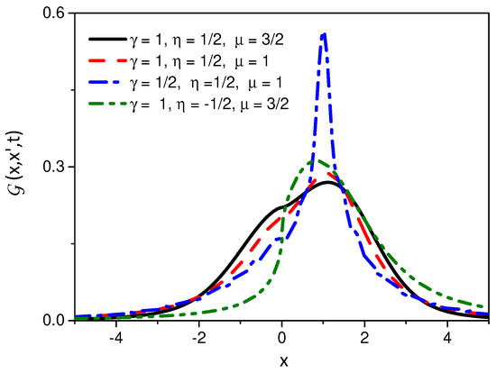
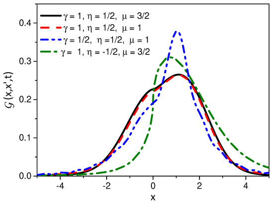
Equation (27) mixing three different parameters, which in connection with a random walk, can be connected to the waiting time and jumping distributions. The parameter $\gamma$ related to the fractional time derivative is connected to the waiting time distribution, and the other parameters $\eta$ and $\mu$ are connected to the jumping probability. We can have a short or a long-tailed behavior for the spatial distribution depending on the choice of the parameter $\eta$ and $\mu$. Figure 1 and Figure 2 show the behavior of ${\mathcal{G}}_{+}(x,x^{\prime },t)$ and ${\mathcal{G}}_{-}(x,x^{\prime },t)$ for different values of the parameters $\gamma$, $\eta$, and $\mu$. In particular, it is possible to observe that depending on the choice of the parameters, the previous Green functions can exhibit a unimodal or a bimodal behavior. Figure 3 shows the behavior of the Green function $\mathcal{G}(x,x^{\prime },t)$ given by Equations (21) and (27). It is worth mentioning that different choices for the parameters imply different behaviors obtained with the mixing of different behaviors.

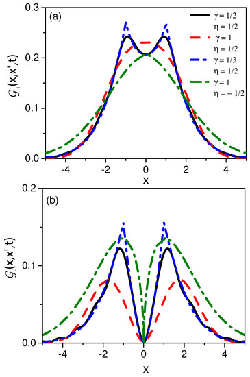
Figure 1. Trend of ${\mathcal{G}}_{+}(x,x^{\prime },t)$ and ${\mathcal{G}}_{-}(x,x^{\prime },t)$ obtained from Equation (22) for $\mu =2$ and different values of $\gamma$ and $\eta$. We consider, for illustrative purposes, ${\chi }_2=1$, $x^{\prime }=1$, and $t=1$. Note that in (a,b) show that ${\mathcal{G}}_{+}(x,x^{\prime },t)$ and ${\mathcal{G}}_{-}(x,x^{\prime },t)$ have different behavior, in particular, near the origin.

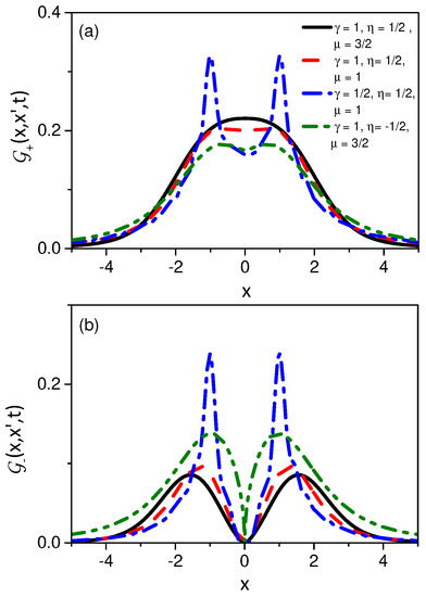
Figure 2. Trend of ${\mathcal{G}}_{+}(x,x^{\prime },t)$ and ${\mathcal{G}}_{-}(x,x^{\prime },t)$ obtained from Equation (27) for different values of $\mu$, $\gamma$ and $\eta$, with $p\left(\overline{\mu }\right)={\chi }_{\mu }\delta (\overline{\mu }-\mu )+{\chi }_2\delta (\overline{\mu }-2)$. We consider, for illustrative purposes, ${\chi }_2=1$, $x^{\prime }=1$, and $t=1$. Note that in (a,b) show that ${\mathcal{G}}_{+}(x,x^{\prime },t)$ and ${\mathcal{G}}_{-}(x,x^{\prime },t)$ have different behavior, in particular, near the origin.

Figure 3. Trend of $\mathcal{G}(x,x^{\prime },t)$ obtained from Equations (21) and (22) for different values of $\mu$, $\gamma$ and $\eta$, with $p\left(\overline{\mu }\right)={\chi }_{\mu }\delta (\overline{\mu }-\mu )$. We consider, for illustrative purposes, ${\chi }_{\mu }=1$, $x^{\prime }=1$, and $t=1$.

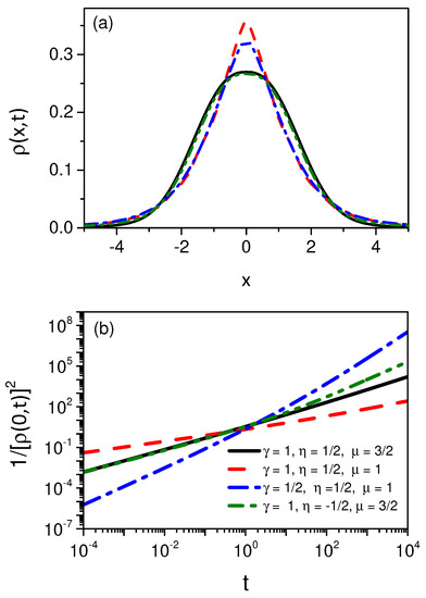
In addition, by using the scaling arguments [13], it is possible to show that the solution can be written as $\rho (x,t)=\rho \left(\xi \right)/t^{\gamma /(\mu +\eta )}$ with $\xi =\left|x\right|/t^{\gamma /(\mu +\eta )}$ and, consequently, ${\sigma }_x^2\sim t^{2\gamma /(\mu +\eta )}$ for ${\int }_{-\infty }^{\infty }d\xi {\xi }^2\rho \left(\xi \right)$ finite. This result implies that for $2\gamma /(\mu +\eta )$ less, equal, or greater than one, we have subdiffusion, usual diffusion, or superdiffusion, respectively (see Figure 4).

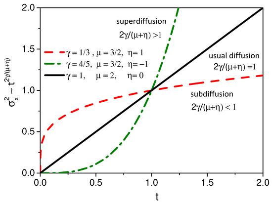
Figure 4. Trend of the mean square displacement ${\sigma }_x^2$ versus t for different values of $\gamma$, $\mu$, and $\eta$. Note that depending on the value of the parameter, different behaviors can be obtained.

Now, we consider the case $p\left(\overline{\mu }\right)={\chi }_2\delta (\overline{\mu }-2)+{\chi }_{\mu }\delta (\overline{\mu }-\mu )$. This case can be connected to the mixing of two different behaviors. For this case, we have that Equation (19) can be written as follows:

$$\begin{array}{c}\hfill {\widehat{\tilde{\mathcal{G}}}}_{\pm }(k,x^{\prime },s)=\frac{1}{2}\frac{{\psi }_{\pm ,\eta }(x^{\prime },k)}{s+s^{1-\gamma }\left({\chi }_2{\left|k\right|}^{2+\eta }+{\chi }_{\mu }{\left|k\right|}^{\overline{\mu }+\eta }\right)}.\end{array}$$

(28)

Applying the inverse of the Laplace transform, we obtain that

$$\begin{array}{ccc}\hfill {\tilde{\mathcal{G}}}_{\pm }(k,x^{\prime },t)& =& \sum _{n=0}^{\infty }\frac{{(-1)}^n}{\Gamma (1+n)}{\left({\chi }_{\mu }{\left|k\right|}^{\mu +\eta }{t}^{\gamma }\right)}^n{E}_{\gamma }^{\left(n\right)}\left({\chi }_2{\left|k\right|}^{2+\eta }{t}^{\gamma }\right)\hfill \\ \hfill & =& \sum _{n=0}^{\infty }\frac{{(-1)}^n}{\Gamma (1+n)}{\left({\chi }_{\mu }{\left|k\right|}^{\mu +\eta }{t}^{\gamma }\right)}^n{\mathrm{H}}_{1,2}^{1,1}\left[{\chi }_2{\left|k\right|}^{2+\eta }{t}^{\gamma }\left|{}_{(0,1),(-\gamma n,\gamma )}^{\left(0,1\right)}\right]\right..\hfill \end{array}$$

(29)

Performing the inverse of the integral transform, we obtain that

$$\begin{array}{ccc}\hfill {\mathcal{G}}_{\pm }(x,x^{\prime },t)& =& \frac{2+\eta }{{2\left|x\right|}^{2+\eta }}{\left(\left|x\right||x^{\prime }|\right)}^{\frac{1}{2}\left(1+\eta \right)}\sum _{n=0}^{\infty }\frac{{(-1)}^n}{\Gamma (1+n)}{\left({\overline{\chi }}_{2,\mu }{t}^{\frac{2-\mu }{\mu +\eta }\gamma }\right)}^n\hfill \\ & \times & {\mathrm{H}}_{2,[0:1],0,[0:2]}^{1,0,1,1,1}\left[\begin{array}{c}{\left(\frac{|x^{\prime }|}{\left|x\right|}\right)}^{2+\eta }\\ \frac{{\overline{\chi }}_2{t}^{\gamma }}{{\left|x\right|}^{2+\eta }}\end{array}\left|\begin{array}{c}\left(\frac{2\mp \nu }{2},1\right);\left(\frac{2\pm \nu }{2},1\right)\\ --;(\frac{2+\eta }{\mu +\eta }n,1)\\ --;--\\ \left(\mp \frac{\nu }{2},1\right);\left(\pm \frac{\nu }{2},1\right);\left(\frac{2+\eta }{\mu +\eta }n,1\right),\left(-\frac{2-\mu }{2+\eta }n\gamma ,\gamma \right)\end{array}\right]\right.,\hfill \end{array}$$

(30)

where ${\overline{\chi }}_{2,\mu }={\chi }_{\mu }/{\chi }_2^{(\mu +\eta )/(2+\eta )}$ and ${\overline{\chi }}_2={(2+\eta )}^2{\chi }_2$.

Figure 5 shows the behavior of the Green function for the previous case, which considers the mixing between two different differential operators.

Figure 5. Trend of $\mathcal{G}(x,x^{\prime },t)$ obtained from Equations (21) and (22) for different values of $\mu$, $\gamma$ and $\eta$, with $p\left(\overline{\mu }\right)={\chi }_{\mu }\delta (\overline{\mu }-\mu )+{\chi }_2\delta (\overline{\mu }-2)$. We consider, for illustrative purposes, ${\chi }_{\mu }=1$, ${\chi }_2=0.6$, $x^{\prime }=1$, and $t=1$.

For the initial condition given by $\rho (x,0)=\delta \left(x\right)$, the solution is illustrated in Figure 6 for different values of the parameters $\gamma$, $\mu$, and $\eta$. We also illustrate the behavior of $1/{\left[\rho (0,t)\right]}^2$, which is connected to the mean square displacement related to this case. In particular, from Figure 6b, it is possible to observe the presence of different diffusion regimes depending on the choice of the parameters.

Figure 6. (a) shows the profile of $\rho (x,t)$ obtained from Equations (15), (21) and (22) for different values of $\mu$, $\gamma$ and $\eta$, with $p\left(\overline{\mu }\right)={\chi }_{\mu }\delta (\overline{\mu }-\mu )$, $t=1$, and $\rho (x,0)=\delta \left(x\right)$. (b) shows the behavior of $1/{\left[\rho (0,t)\right]}^2$ to illustrate the spreading of the system. We consider, for illustrative purposes, ${\chi }_{\mu }=1$ and $t=1$.

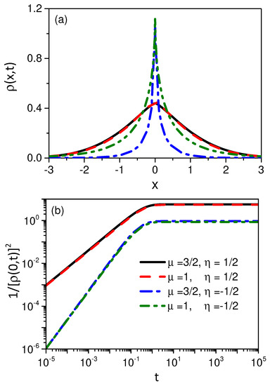
We can consider a different fractional time operator for the previous scenarios defined by Equation (14). One of them is the Caputo–Fabrizio fractional operator [28]. In this case, Equation (14) can be written as follows:

$$\begin{array}{c}\hfill \frac{\partial }{\partial t}\rho (x,t)={\int }_0^{\mu }d\overline{\mu }p\left(\overline{\mu }\right)D_x^{\overline{\mu },\eta }\rho (x,t)+r\left(\delta (x-x^{\prime })-\rho (x,t)\right),\end{array}$$

(31)

with $r=\gamma /(1-\gamma )$, for the initial condition $\rho (x,0)=\delta (x-x^{\prime })$. It is worth mentioning that Equation (31) corresponds to a system subjected to a stochastic resetting [61]. In particular, it extends the processes described in Ref. [56]. By using the previous approach, it is possible to show that the solution for this case is given by

$$\begin{array}{c}\hfill \rho (x,t)=e^{-rt}\mathcal{G}(x,x^{\prime },t)+r{\int }_0^{t}d{t}^{\prime }{e}^{-r{t}^{\prime }}\mathcal{G}(x,x^{\prime },t^{\prime })\end{array}$$

(32)

with the Green function given by Equations (21) and (27). For the particular case, $p\left(\overline{\mu }\right)={\chi }_{\mu }\delta (\overline{\mu }-\mu )$ with $x^{\prime }=0$, we have that the Green function is given by

$$\begin{array}{c}\hfill \mathcal{G}(x,0,t)=\frac{2+\eta }{2(\mu +\eta )\left|x\right|\Gamma \left(\frac{3+\eta }{2+\eta }\right)}{\mathrm{H}}_{2,3}^{2,1}[\frac{{\left|x\right|}^{2+\eta }}{{(2+\eta )}^2{\left({\chi }_{\mu }{t}^{\gamma }\right)}^{\frac{2+\mu }{2+\eta }}}\left|{}_{\left(\frac{1}{2+\eta },1\right),\left(1,\frac{2+\eta }{\mu +\eta }\right),\left(1,1\right)}^{\left(1,\frac{2+\eta }{\mu +\eta }\right),\left(1,\frac{2+\eta }{\mu +\eta }\right)}]\right..\end{array}$$

(33)

Figure 7a shows the behavior of Equation (32) and Figure 7b shows the behavior of $1/{\left[\rho (0,t)\right]}^2$ to illustrate the spreading of the system for different values of the parameters $\eta$ and $\mu$ with $\gamma =1/2$. From this figure, we observe that the system has long been stationary. It is also interesting to mention that Equation (32) with the Green function given by Equation (33) allows us to investigate a diffusive process in heterogeneous media with stochastic resetting.

Figure 7. (a) shows the profile of $\rho (x,t)$ obtained from Equations (31) and (33) for different values of $\mu$, $\gamma$ and $\eta$, with $p\left(\overline{\mu }\right)={\chi }_{\mu }\delta (\overline{\mu }-\mu )$, $t=1$, and $\rho (x,0)=\delta \left(x\right)$. (b) shows the behavior of $1/{\left[\rho (0,t)\right]}^2$ to illustrate the spreading of the system. We consider, for illustrative purposes, ${\chi }_{\mu }=1$ and $r=1$.

Now, we consider the presence of a non-local term in the diffusion equation. We also consider, for simplicity, the initial condition $\rho (x,0)=\delta \left(x\right)$, $p\left(\overline{\mu }\right)={\chi }_{\mu }\delta (\overline{\mu }-\mu )$, and the Riemann–Liouville fractional time operator. For this case, we can apply the previous procedure based on integral transforms, yielding

$$\begin{array}{c}\hfill {\widehat{\tilde{\rho }}}_{+}(k,s)=\frac{1}{2}\frac{{\psi }_{+}(0,k)}{s+s^{1-\gamma }{\chi }_{\mu }{\left|k\right|}^{\mu }+\Lambda \left(s\right)}.\end{array}$$

(34)

After performing a series of expansions, we have that

$$\begin{array}{c}\hfill {\widehat{\tilde{\rho }}}_{+}(k,s)=\frac{1}{2}\frac{{\psi }_{+}(0,k)}{s+s^{1-\gamma }{\chi }_{\mu }{\left|k\right|}^{\mu }}\sum _{n=0}^{\infty }{(-1)}^n{\left[\frac{\Lambda \left(s\right)}{s+s^{1-\gamma }{\chi }_{\mu }{\left|k\right|}^{\mu }}\right]}^n,\end{array}$$

(35)

which, after performing the inverse integral transforms, yields

$$\begin{array}{ccc}\hfill \rho (x,t)& =& {\mathcal{G}}_{+}(x,0,t)+\sum _{n=1}^{\infty }{\left(-\frac{1}{2}\right)}^n{\int }_0^{t}d{t}_n{\int }_{-\infty }^{\infty }d{x}_n\mathsf{{\rm Y}}(x,x_n,t-t_n)\cdots \hfill \\ & \times & {\int }_0^{t_2}d{t}_1{\int }_{-\infty }^{\infty }{d}_{x_2}\mathsf{{\rm Y}}(x_2,x_1,t_2-t_1)\mathsf{{\rm Y}}(x_1,0,t_1)\hfill \end{array}$$

(36)

where $\mathsf{{\rm Y}}(x,\xi ,t)={\int }_0^{t}d{t}^{\prime }{\mathcal{G}}_{+}(x,\xi ,t-t^{\prime })\Lambda \left(t^{\prime }\right)$.

3. Discussion and Conclusions

We have investigated a generalized diffusion equation which has, in particular cases, several situations. We have started our analysis by considering the fractional spatial operator and analyzed the influence of the fractional time operators on the solutions. In this scenario, we have obtained the time behavior of the mean square displacement by using scaling arguments when fractional space and time derivatives are present in the diffusion equation. In this case, we consider a singular kernel for the fractional time derivative that allows a connection with the Riemann–Liouville fractional time derivative. For the spatial fractional operator, we have also considered an operator of distributed order. In particular, we analyzed the mixing between two cases, i.e., $p\left(\overline{\mu }\right)={\chi }_{\mu }\delta (\overline{\mu }-\mu )+{\chi }_2\delta (\mu -2)$. In each case, the solutions can be directly connected to the stretched exponential or power laws, depending on the choice of the parameters characterizing the spatial fractional operator. We have also considered Fabrizio–Caputo fractional time operator. For this case, we have related this case with a stochastic resetting process following the approach presented in Ref. [28] and analyzed the behavior of the solutions. For each case, the solutions were obtained using the Green function approach. In addition, we have also considered the solutions for an arbitrary non-local term in the generalized diffusion equation. Finally, we hope that the results found here can be helpful in the discussion of different scenarios in connection with diffusion and anomalous diffusion processes.

References

- Hilfer, R. Applications of Fractional Calculus in Physics; World Scientific: Singapore, 2000. [Google Scholar]
- Meerschaert, M.M.; Sikorskii, A. Stochastic Models for Fractional Calculus; de Gruyter: Berlin, Germany, 2019. [Google Scholar]
- Tarasov, V.E. Fractional Dynamics: Applications of Fractional Calculus to Dynamics of Particles, Fields and Media; Springer Science & Business Media: Berlin, Germany, 2011. [Google Scholar]
- Magin, R. Fractional calculus in bioengineering, part 1. Crit. Rev. Biomed. Eng. 2004, 32, 1–104. [Google Scholar] [CrossRef] [PubMed]
- Herrmann, R. Fractional Calculus: An Introduction for Physicists; World Scientific: Singapore, 2011. [Google Scholar]
- Evangelista, L.R.; Lenzi, E.K. Fractional Diffusion Equations and Anomalous Diffusion; Cambridge University Press: Cambridge, UK, 2018. [Google Scholar]
- Kuntz, M.; Lavallée, P. Experimental evidence and theoretical analysis of anomalous diffusion during water infiltration in porous building materials. J. Phys. D Appl. Phys. 2001, 34, 2547. [Google Scholar] [CrossRef]
- Rosseto, M.P.; Evangelista, L.R.; Lenzi, E.K.; Zola, R.S.; Ribeiro de Almeida, R.R. Frequency-Dependent Dielectric Permittivity in Poisson–Nernst–Planck Model. J. Phys. Chem. B 2022, 126, 6446–6453. [Google Scholar] [CrossRef]
- Scher, H.; Montroll, E.W. Anomalous transit-time dispersion in amorphous solids. Phys. Rev. B 1975, 12, 2455. [Google Scholar] [CrossRef]
- Jeon, J.H.; Leijnse, N.; Oddershede, L.B.; Metzler, R. Anomalous diffusion and power-law relaxation of the time averaged mean squared displacement in worm-like micellar solutions. New J. Phys. 2013, 15, 045011. [Google Scholar] [CrossRef]
- Metzler, R.; Klafter, J. The random walk’s guide to anomalous diffusion: A fractional dynamics approach. Phys. Rep. 2000, 339, 1–77. [Google Scholar] [CrossRef]
- Lenzi, E.K.; Evangelista, L.; Zola, R.; Scarfone, A. Fractional Schrödinger equation for heterogeneous media and Lévy-like distributions. Chaos Solitons Fractals 2022, 163, 112564. [Google Scholar] [CrossRef]
- Magin, R.L.; Lenzi, E.K. Slices of the Anomalous Phase Cube Depict Regions of Sub-and Super-Diffusion in the Fractional Diffusion Equation. Mathematics 2021, 9, 1481. [Google Scholar] [CrossRef]
- Kenkre, V.; Montroll, E.; Shlesinger, M. Generalized master equations for continuous-time random walks. J. Stat. Phys. 1973, 9, 45–50. [Google Scholar] [CrossRef]
- Swenson, R.J. Derivation of generalized master equations. J. Math. Phys. 1962, 3, 1017–1022. [Google Scholar] [CrossRef]
- Cortes, E.; West, B.J.; Lindenberg, K. On the generalized Langevin equation: Classical and quantum mechanicala. J. Chem. Phys. 1985, 82, 2708–2717. [Google Scholar] [CrossRef]
- Klafter, J.; Sokolov, I.M. First Steps in Random Walks: From Tools to Applications; OUP Oxford: Oxford, UK, 2011. [Google Scholar]
- Giona, M.; Roman, H.E. Fractional diffusion equation on fractals: One-dimensional case and asymptotic behaviour. J. Phys. A Math. Gen. 1992, 25, 2093. [Google Scholar] [CrossRef]
- Hashan, M.; Jahan, L.N.; Imtiaz, S.; Hossain, M.E. Modelling of fluid flow through porous media using memory approach: A review. Math. Comput. Simul. 2020, 177, 643–673. [Google Scholar] [CrossRef]
- Razminia, K.; Razminia, A.; Baleanu, D. Fractal-fractional modelling of partially penetrating wells. Chaos Solitons Fractals 2019, 119, 135–142. [Google Scholar] [CrossRef]
- Raghavan, R.; Chen, C. The Theis solution for subdiffusive flow in rocks. Oil Gas Sci. Technol. Rev. D’Ifp Energies Nouv. 2019, 74, 6. [Google Scholar] [CrossRef]
- Zhokh, A.; Strizhak, P. Macroscale modeling the methanol anomalous transport in the porous pellet using the time-fractional diffusion and fractional Brownian motion: A model comparison. Commun. Nonlinear Sci. Numer. Simul. 2019, 79, 104922. [Google Scholar] [CrossRef]
- Feng, C.; Si, X.; Li, B.; Cao, L.; Zhu, J. An inverse problem to simulate the transport of chloride in concrete by time–space fractional diffusion model. Inverse Probl. Sci. Eng. 2021, 29, 2429–2445. [Google Scholar] [CrossRef]
- Han, M.; Zhou, C.; Silberschmidt, V.V.; Bi, Q. Multiscale heat conduction and fractal oxidation behaviors of needle-punched carbon/carbon composites. Sci. Eng. Compos. Mater. 2022, 29, 508–515. [Google Scholar] [CrossRef]
- Lenzi, E.K.; Evangelista, L. Space–time fractional diffusion equations in d-dimensions. J. Math. Phys. 2021, 62, 083304. [Google Scholar] [CrossRef]
- Podlubny, I. Fractional Differential Equations; Academic Press: Cambridge, MA, USA, 1999. [Google Scholar]
- Atangana, A.; Baleanu, D. New Fractional Derivatives with non-local and non-singular kernel. Therm. Sci. 2016, 20, 763–769. [Google Scholar] [CrossRef]
- Tateishi, A.A.; Ribeiro, H.V.; Lenzi, E.K. The role of fractional time-derivative operators on anomalous diffusion. Front. Phys. 2017, 5, 52. [Google Scholar] [CrossRef]
- Fernandez, A.; Baleanu, D. Classes of operators in fractional calculus: A case study. Math. Methods Appl. Sci. 2021, 44, 9143–9162. [Google Scholar] [CrossRef]
- Singh, H. Chebyshev spectral method for solving a class of local and nonlocal elliptic boundary value problems. Int. J. Nonlinear Sci. Numer. Simul. 2021. [Google Scholar] [CrossRef]
- Singh, H. Solving a class of local and nonlocal elliptic boundary value problems arising in heat transfer. Heat Transf. 2022, 51, 1524–1542. [Google Scholar] [CrossRef]
- Singh, H. An efficient computational method for non-linear fractional Lienard equation arising in oscillating circuits. In Methods of Mathematical Modelling; CRC Press: Boca Raton, FL, USA, 2019; pp. 39–50. [Google Scholar]
- Singh, H.; Srivastava, H. Numerical investigation of the fractional-order Liénard and Duffing equations arising in oscillating circuit theory. Front. Phys. 2020, 8, 120. [Google Scholar] [CrossRef]
- Scarfone, A.M.; Barbero, G.; Evangelista, L.R.; Lenzi, E.K. Anomalous Diffusion and Surface Effects on the Electric Response of Electrolytic Cells. Physchem 2022, 2, 163–178. [Google Scholar] [CrossRef]
- Barbero, G.; Evangelista, L.; Lenzi, E.K. Time-fractional approach to the electrochemical impedance: The Displacement current. J. Electroanal. Chem. 2022, 920, 116588. [Google Scholar] [CrossRef]
- Singh, H.; Srivastava, H.; Nieto, J.J. Handbook of Fractional Calculus for Engineering and Science; CRC Press: Boca Raton, FL, USA, 2022. [Google Scholar]
- Singh, H.; Kumar, D.; Baleanu, D. Methods of Mathematical Modelling: Fractional Differential Equations; CRC Press: Boca Raton, FL, USA, 2019. [Google Scholar]
- Singh, H.; Kumar, D.; Baleanu, D. Methods of Mathematical Modelling: Infectious Disease; Elsevier Science: Amsterdam, The Netherlands, 2022. [Google Scholar]
- Gómez-Aguilar, J.; Atangana, A. Fractional Hunter-Saxton equation involving partial operators with bi-order in Riemann–Liouville and Liouville–Caputo sense. Eur. Phys. J. Plus 2017, 132, 100. [Google Scholar] [CrossRef]
- Evangelista, L.R.; Lenzi, E.K. An Introduction to Anomalous Diffusion and Relaxation; Springer Nature: Berlin, Germany, 2023. [Google Scholar]
- Ali, I.; Kalla, S. A generalized Hankel transform and its use for solving certain partial differential equations. Anziam J. 1999, 41, 105–117. [Google Scholar] [CrossRef]
- Garg, M.; Rao, A.; Kalla, S.L. On a generalized finite Hankel transform. Appl. Math. Comput. 2007, 190, 705–711. [Google Scholar] [CrossRef]
- Nakhi, Y.B.; Kalla, S.L. Some boundary value problems of temperature fields in oil strata. Appl. Math. Comput. 2003, 146, 105–119. [Google Scholar] [CrossRef]
- Xie, K.; Wang, Y.; Wang, K.; Cai, X. Application of Hankel transforms to boundary value problems of water flow due to a circular source. Appl. Math. Comput. 2010, 216, 1469–1477. [Google Scholar] [CrossRef]
- O’Shaughnessy, B.; Procaccia, I. Diffusion on fractals. Phys. Rev. A 1985, 32, 3073–3083. [Google Scholar] [CrossRef]
- O’Shaughnessy, B.; Procaccia, I. Analytical Solutions for Diffusion on Fractal Objects. Phys. Rev. Lett. 1985, 54, 455–458. [Google Scholar] [CrossRef]
- Richardson, L.F. Atmospheric diffusion shown on a distance-neighbour graph. Proc. Math. Phys. Eng. Sci. 1926, 110, 709–737. [Google Scholar]
- Boffetta, G.; Sokolov, I.M. Relative Dispersion in Fully Developed Turbulence: The Richardson’s Law and Intermittency Corrections. Phys. Rev. Lett. 2002, 88, 094501. [Google Scholar] [CrossRef]
- Ben Avraham, D.; Havlin, S. Diffusion and Reactions in Fractals and Disordered Systems; CUP: Cambridge, UK, 2000. [Google Scholar]
- Su, N.; Sander, G.; Liu, F.; Anh, V.; Barry, D. Similarity solutions for solute transport in fractal porous media using a time- and scale-dependent dispersivity. App. Math. Model. 2005, 29, 852–870. [Google Scholar] [CrossRef]
- He, J.H. Fractal calculus and its geometrical explanation. Results Phys. 2018, 10, 272–276. [Google Scholar] [CrossRef]
- Cai, W.; Chen, W.; Xu, W. The fractal derivative wave equation: Application to clinical amplitude/velocity reconstruction imaging. J. Acoust. Soc. Am. 2018, 143, 1559–1566. [Google Scholar] [CrossRef]
- Chen, W.; Liang, Y. New methodologies in fractional and fractal derivatives modeling. Chaos Solitons Fractals 2017, 102, 72–77. [Google Scholar] [CrossRef]
- Liang, Y.; Chen, W.; Cai, W. Hausdorff Calculus: Applications to Fractal Systems; Walter de Gruyter GmbH & Co KG: Berlin, Germany, 2019; Volume 6. [Google Scholar]
- Evans, M.R.; Majumdar, S.N. Diffusion with stochastic resetting. Phys. Rev. Lett. 2011, 106, 160601. [Google Scholar] [CrossRef] [PubMed]
- Lenzi, M.K.; Lenzi, E.K.; Guilherme, L.; Evangelista, L.R.; Ribeiro, H.V. Transient anomalous diffusion in heterogeneous media with stochastic resetting. Phys. A Stat. Mech. Appl. 2022, 588, 126560. [Google Scholar] [CrossRef]
- Wyld, H.W.; Powell, G. Mathematical Methods for Physics; CRC Press: Boca Raton, FL, USA, 2020. [Google Scholar]
- Mathai, A.M.; Saxena, R.K.; Haubold, H.J. The H-Function: Theory and Applications; Springer Science & Business Media: Berlin, Germany, 2009. [Google Scholar]
- Lenzi, E.K.; Evangelista, L.; Lenzi, M.K.; Ribeiro, H.V.; de Oliveira, E.C. Solutions for a non-Markovian diffusion equation. Phys. Lett. A 2010, 374, 4193–4198. [Google Scholar] [CrossRef]
- Jiang, X.; Xu, M. The time fractional heat conduction equation in the general orthogonal curvilinear coordinate and the cylindrical coordinate systems. Phys. A Stat. Mech. Appl. 2010, 389, 3368–3374. [Google Scholar] [CrossRef]
- Evans, M.R.; Majumdar, S.N.; Schehr, G. Stochastic resetting and applications. J. Phys. A 2020, 53, 193001. [Google Scholar] [CrossRef]
Disclaimer/Publisher’s Note: The statements, opinions and data contained in all publications are solely those of the individual author(s) and contributor(s) and not of MDPI and/or the editor(s). MDPI and/or the editor(s) disclaim responsibility for any injury to people or property resulting from any ideas, methods, instructions or products referred to in the content. |
© 2023 by the authors. Licensee MDPI, Basel, Switzerland. This article is an open access article distributed under the terms and conditions of the Creative Commons Attribution (CC BY) license (https://creativecommons.org/licenses/by/4.0/).