Abstract
This paper analyses the stability of thin power-law fluid flowing down a moving plane in a vertical direction by using the long-wave perturbation method. Linear and nonlinear stability are discussed. The linear stable region increases as the downward speed increases and the power-law index increases. More accurate results are obtained on the coefficients of the nonlinear generalized kinematic equation in the power-law part. The regions of sub-critical instability and absolute stability are expanded when the downward movement of plane increases, or the power-law index increases, and meanwhile the parts of supercritical stability and explosive supercritical instability are compressed. By substituting the power-law index and moving speed into the generalized nonlinear kinematic equation of the power-law film on the free surface, the results can be applied to estimate the stability of the thin film flow in the field of engineering.
1. Introduction
Generally, fluid has two different flow states. According to experience, the Reynolds number can be used to determine whether the flow is laminar or turbulent, and it is relatively easy to use. However, this method is not an exact indicator of whether the fluid is actually laminar or turbulent. In general, a fluid will exhibit laminar flow at a lower Reynolds number, where the disturbance can be dissipated through the viscous effect of the fluid, and thus remain in a laminar flow state, which is called stability. Once a small disturbance in the laminar flow grows so large that the entire flow state is changed then the fluid loses its stability and enters the turbulent state. A system needs to be stable under all disturbance conditions in order to be in a stable state. By discussing the stability of the fluid, we can determine whether the fluid is laminar or turbulent, and we can understand under what conditions the flow will lose its stability.
The discussion of fluid stability is a relatively old topic. The stability of fluids is also discussed in books written by Lin [1] and Chandrasekhar [2]. For the stability of the fluid film, it was first assumed in the paper by Kapitza [3] in 1949 that a velocity distribution was considered in the boundary layer equation and the momentum integral method was applied to the boundary layer equation. Nonlinear stability was mostly ignored in the discussion of fluid stability because the nonlinear theory had some obvious defects. Since 1960, there have been more and more nonlinear theories that have improved the whole theory of fluid stability. Landau, who has contributed so much to hydrodynamic stability, proposed the Landau equation. Then, the nonlinear free-surface equation of thin-film fluid was derived by using Benney’s [4] small parameter expansion method. Lin [5], Nakaya [6], and Krishna [7] used this method to derive the Landau equation, which shows that the nonlinear instability occurs near the linear neutral curve. The stability of film flow on a flat plane has been researched by many scholars. This paper follows the previous small parameter expansion method.
In recent years, there have been more and more studies and discussions of thin film fluids, and such issues have attracted more and more attention from scholars. Tsai [8] discussed the linear stability problem of thin magnetic fluid films condensing on a flat plane. Lai [9] discussed the stability of Newtonian fluid films on a vertical moving plane. Naganthran [10,11] focused on the Carreau thin film flow over an unsteady stretching sheet and provided several different numerical solutions. After that, Naganthran [12] presented a melting heat transfer and entropy analysis about the Carreau thin hybrid nanofluid film flow past a stretching sheet.
The topic of non-Newtonian fluid makes the stability of film flow more complex. Correspondingly, there are more research efforts in the direction of non-Newtonian fluids. Rehman [13,14] discussed the numerical calculation of flow through obstacles for two different non-Newtonian fluids, Eyring–Power fluid and Carreau–Bird law fluid. The results show that the effect of non-Newtonian fluids cannot be ignored. Cheng [15,16] discussed the film stability of a pseudoplastic fluid and a viscoelastic fluid on a vertical plane. Amaouche [17] discussed the linear stability of a power-law fluid film flowing down an inclined plane. The rupture problem of a thin micropolar liquid film under a magnetic field on a horizontal plane was investigated by Cheng [18]. Some other geometric models of power-law film flow are discussed. Lin [19] discussed the linear stability of a pseudoplastic fluid with condensation effects flowing on a rotating circular disk. Chen [20] derived the nonlinear stability of a thin micropolar film falling exterior to a rotating vertical cylinder. Lin [21] examines the hydromagnetic weakly nonlinear stability of a general viscous fluid film flow on a rotating vertical cylinder. These studies continue to broaden the use of thin film stability analysis. The goal of this article is to further expand the current range of use so that the stability analysis can also be used on power-law fluid film flow on a moving plane.
It is very difficult to construct an experiment that can accurately measure the flow state of a fluid, and the measurement itself is usually quite hard. So, most of the research on fluid stability is based on mathematical modeling and theoretical demonstration. It is very important to discuss the stability of fluid to solve engineering problems. The mathematical model of laminar or turbulent flow can be confirmed after the fluid state is determined. The study of hydrodynamic stability becomes more complicated because of the properties of non-Newtonian fluid.
An important process in the automotive industry is to paint the surface of a car. A lot of the paintwork in the modern automobile industry is carried out by immersing the frame of the car into a paint tank and then taking it out. The paint will form a coating layer along the surface of the frame. It is important to understand the relation between the flow state of the coating and how it affects the coating formation and the flow stability of the coating film on the frame surface.
Using the process of coating a car frame as an example, the paint is a non-Newtonian fluid, and the frame itself has motion relative to the paint pool that is similar to the movement of plane motion in a non-Newtonian fluid. In this paper, the power-law fluid film is the main object of this research, and the stability of the flow state on the movable plane surface is discussed. The small parameter expansion method is applied in the case where the surface wavelength of the thin film is much longer than the thickness of the liquid film. The linear and nonlinear stability analysis of a power-law fluid film flowing on a moving wall is discussed in this paper.
2. Generalized Kinematic Equation
The simplified model of this study is shown in Figure 1. It shows a thin power-law film flow down and along a vertically moving plane. U* is the moving velocity of the plate in vertical direction, h* is the film thickness, h0* is the film thickness in equilibrium state, u0* is reference velocity. The research focuses on the hydrodynamic stability of the power-law fluid film affected by a small perturbation when the fluid is in a steady-state equilibrium at first. Consider the surface tension and density of the fluid as constant. The power-law fluid which uses the Ostwald–de Waele model obeys the constitutive equation of state [22].
where is the stress tensor, is the isotropic pressure, is the dynamic viscosity of power-law fluid, and is the rate of the strain tensor. can be defined as
where n is the power-law index of the fluid, and u* and v* are the velocity components in x* and y* directions, respectively. Assume that the flow is isothermal and incompressible. The governing equation of mass and momentum can be expressed in terms of Cartesian coordinates as
where ρ is a constant density of the fluid, t* is the time, and g is the gravitational acceleration. The individual stress components can be written as
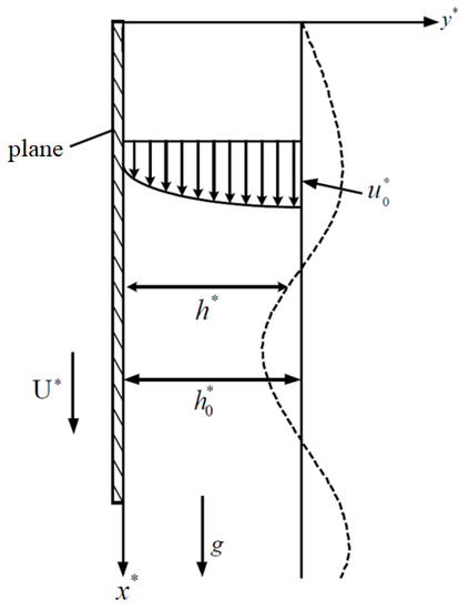
Figure 1.
Schematic diagram of a thin power-law fluid film flowing down a moving plane in a vertical direction.
The boundary condition on the wall () obeys the no-slip condition
where U* is the moving velocity of the vertical plane. The boundary condition for the free surface at () is derived based on the result given by Edwards et al. [23] The shear stress for film flow at the free surface is given as
The normal stress for film flow at the free surface is given as
The kinematic boundary condition, which means the velocity directly perpendicular to the free surface must vanish on the boundary itself, can be expressed as
where h* is the local film thickness, Pa* is the atmosphere pressure, and S* is the surface tension. The variable associated with a superscript ‘*’ stands for a dimensional quantity. By introducing the stream function φ*, the dimensional velocity components can be expressed as
In order to make the equations dimensionless, the variables in the equations can be defined as
where α is the dimensionless wave number, h0* is the film thickness of local base flow, u0* is the reference velocity, Ren is the Reynolds number, and λ is the perturbation wavelength. The moving velocity of the vertical plane, which can be denoted as U*, can be expressed as
where Z is a specific constant ratio of the plane velocity to the free stream velocity, and ν is the kinematic viscosity of power-law fluid. The reference velocity u0* can be expressed as
Thus the dimensionless governing equations can be expressed as
and associated boundary conditions on the wall surface () can be given as
The boundary conditions at the free surface () of the film flow can be given as
Subscripts of t, x, and y are used to represent the associated partial derivatives of the underlying variable. The film flow will be a classical Newtonian flow if the power-law index n = 1.
Since the long-wavelength models that give the smallest wave number are most likely to induce flow instability for the film flow, the above equations can be computed by expanding the stream function and pressure in terms of small wave number as
By plugging the above two equations into Equations (15)–(21), the governing equations can be expanded order by order. Since the non-dimensional surface tension S is a large value in practice, the term α2S can then be treated as a quantity of zeroth order. After collecting all terms of zeroth order in the governing equations, a set of zeroth-order equations can be obtained
The boundary conditions associated with the equations of zeroth order are given as
Thus, the solution of the zeroth-order equations is
The first order governing equations are given as
and the boundary conditions associated with the equations of the first order are given as
The value of power-law index n is near 1 and is a small number, so in Equation (30) is approximated to 1. By plugging the zeroth-order solutions into the first-order equations and boundary conditions, the first-order solution of the stream function can be given as
By plugging the solutions for the equations of both the zeroth and the first orders into the dimensionless free surface kinematic equation of Equation (21), the nonlinear generalized kinematic equation can be obtained and presented as
where
In the case of n = 1, the film flow is equal to the Newtonian fluid. The equations above have been carefully derived and presented by Lai et al. [8]. They are more accurate than the results from Cheng [15].
2.1. Stability Analysis
The dimensionless film thickness in the perturbed state can be written as
where η is the perturbation quantity of the stationary film thickness. By inserting Equation (41) into Equation (35) and collecting all terms up to the order of three, the equation of η can be written as
where the values of A, B, C, D, E, and their derivatives are evaluated at the dimensionless height, h = 1, of the film.
2.2. Linear Stability Analysis
To analyze the linear stability of the film flow, the nonlinear terms in Equation (42) should be assumed insignificant and neglected. Then, Equation (42) can be given as
The normal mode analysis is performed by assuming that
where a is the perturbation amplitude, and c.c. is the complex conjugate counterpart. The complex wave celerity, d, can be given as
where dr is the linear wave speed, and di is the linear growth rate of the wave amplitudes. The characterization of flow stability is under linearly unstable supercritical condition for di > 0, and it is under linearly stable subcritical condition for di < 0.
2.3. Weakly Nonlinear Stability Analysis
Considering the nonlinear effect, the perturbation is assumed as a small wave that does not fundamentally alter the nature of the motion. The multiple scales method is used to characterize the weakly nonlinear behaviors of the fluid. The resulting Ginburg–Landau equation [24] can be derived following the same procedure as Cheng [9] and Lai [8]:
where
The overhead bar appearing in Equation (46) stands for the complex conjugate of the same variable. The solution of the Ginburg–Landau equation can be assumed as
By substituting Equation (51) into Equation (46), the result can be expressed as
The associated wave amplitude is given as
The nonlinear wave speed of the supercritical stable region is given as
Equations (52)–(55) are used to determine the stability state of the film fluid. The criteria for stability are presented in Table 1.

Table 1.
Various states of the Landau equation.
3. Numerical Results and Discussions
It can be explained more clearly by giving an example using a specific numerical model. Take the stability behavior of the thin power-law fluid film flowing down a moving plane in a vertical direction as an example. The power-law index of common fluids generally ranges around 1. The value of Z is the velocity ratio, which is presented in Table 2. This study will use the following physical quantities for calculation: Reynolds numbers (Re) are from 0 to 15; the dimensionless perturbation wave numbers (α) are from 0 to 0.12; the value of constant dimensionless surface tension is set to 6173.5 [10]; the velocity ratio (Z) is set to −0.32, 0, 0.51; and the power-law index (n) is set to 0.95, 1, 1.05.
Table 2.
The corresponding value of Z at various plane movement speeds.
3.1. Linear Stability Analysis
The linear stability of film flow can be determined by the term di in Equation (45), which is the linear growth rate of the wave amplitude. Figure 2 shows the region is divided into two parts by the linear neutral curve di = 0.
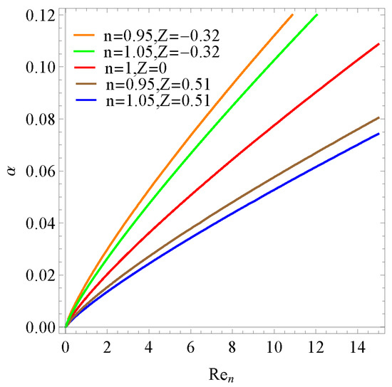
Figure 2.
Neutral linear stability curves of the film flow for various n and Z.
The part on the left of the curve is di < 0, and in this part, the flow will remain stable when it encounters disturbance. The perturbation will gradually disappear by the viscous effect, and the flow will stay in laminar flow. The flow will be unstable on the right side of the curve. The perturbation will grow stronger and be able to change the laminar flow into a turbulent flow. Figure 2 shows the neutral stability curve of Newtonian film fluid on the stationary wall and two kinds of non-Newtonian fluid under two wall speed on two sides.
When the plane moves downward (z > 0), the neutral stability curve will shift to the right, which means the range of the fluid in the stable condition increases; on the contrary, when the plane moves upward (z < 0), the neutral stability curve will shift to the left, which means the range of the fluid in the unstable condition increases, and the fluid is more likely to become unstable. When the power-law index of the non-Newtonian fluid (n) is greater than 1, the curve will shift to the right, and the range of the fluid in the stable condition increases accordingly. On the contrary, when the power-law index (n) is less than 1, the curve will shift to the left, and the range of the fluid in unstable conditions increases accordingly. Overall, the increase in the power-law index n and the movement downward will promote the fluid to be stable.
Due to the fact that stability will be influenced by both n and Z, we chose the condition of n = 1.05 and Z = 0.51, n = 0.95and Z = −0.32 in order to make the chart clearer.
Figure 3 shows the variation of the temporal amplitude growth rate of non-Newtonian fluid film on different moving planes with dimensionless wave number α under the condition of Re = 10. It can be seen that the temporal amplitude growth rate reaches 0 faster when the downward movement is more acute and the power-law index n is larger.
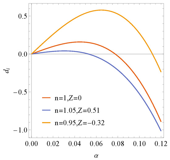
Figure 3.
Linear amplitude growth rate of disturbed waves for various n and Z at Re = 10.
Figure 4 shows the variation of the temporal amplitude growth rate of non-Newtonian fluid film on different moving planes with Re under the condition of dimensionless wave number α = 0.06. For the same Re, it can be seen that the temporal amplitude growth rate reaches 0 faster when the downward movement is more acute and the power-law index n is also larger.
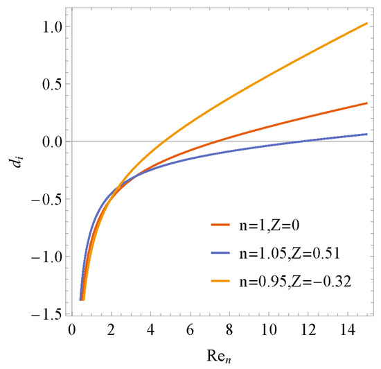
Figure 4.
Linear amplitude growth rate of disturbed waves for various n and Z at α = 0.06.
3.2. Nonlinear Stability Analysis
As the amplitude of the perturbation wave increases, the nonlinear effect cannot be neglected. By using the weakly nonlinear stability analysis, the various states of the flow are shown in Table 1. The stability states can be determined by di and E1. If E1 > 0, the nonlinear effect will promote the film fluid to become stable. On the other side, if the E1 < 0, the nonlinear effect will promote the film to become unstable.
There are 4 types of conditions, which are sub-critical instability, subcritical stability, supercritical stability, and explosive supercritical instability.
The regions of Figure 5, Figure 6 and Figure 7 are separated by the blue curves and orange curves. The blue curve is di = 0. The orange curve is E1 = 0. Figure 6 shows the result of the growth amplitude of the Newtonian fluid film flowing down along a vertical static plane. This figure is separated into four parts which are the four types of the condition by the curve di = 0 and E1 = 0. By comparing the results of Figure 5, n = 1.05 Z = 0.51, and Figure 7, n = 0.95 Z = −0.32, with Figure 6, the following can be concluded: the regions of sub-critical instability and absolute stability are expanded; meanwhile, the parts of supercritical stability and explosive supercritical instability are compressed when the plane moves downward, Z > 0, or the power-law index n > 1. The parts of sub-critical instability and absolute stability are compressed; meanwhile, the parts of supercritical stability and explosive supercritical instability are expanded when the plane moves upward, Z < 0, or the power-law index n < 1. Z increases or power-law index n increases has similar influences on the stability, but the specific behaviors are different. It can be calculated by substituting Z, n into Equations (35)–(40).
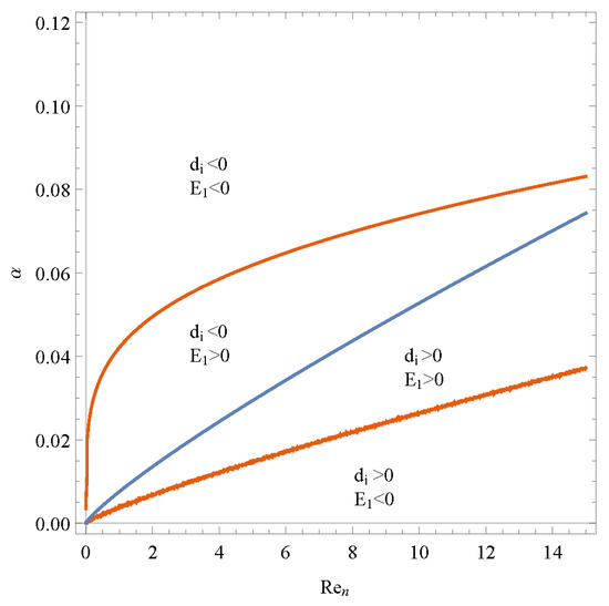
Figure 5.
Nonlinear neutral stability curves of the film flow for various α and Re at n = 1.05, Z = 0.51.
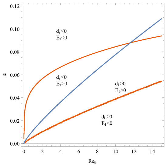
Figure 6.
Nonlinear neutral stability curves of the film flow for various α and Re at n = 1, Z = 0.
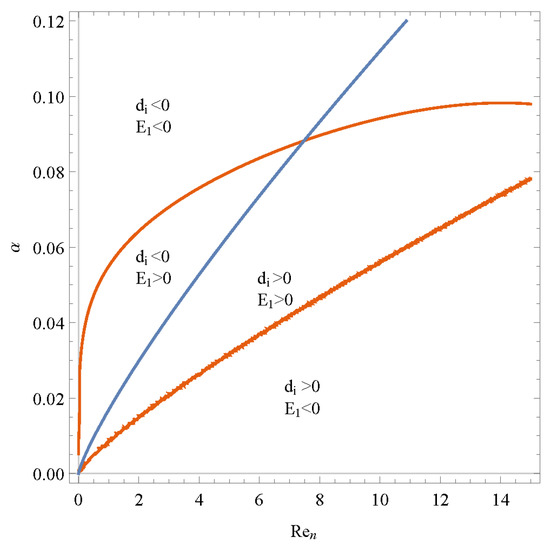
Figure 7.
Nonlinear neutral stability curves of the film flow for various α and Re at n = 0.95, Z = −0.32.
Figure 8 shows how the nonlinear threshold amplitude at Re = 5 will be affected by different plane movement speeds and power-law index values while α varies from 0.08 to 0.12, which is in the subcritical unstable region. The threshold amplitude curves cross near α = 0.09. This is quite different from the result only influenced by plane movement or the non-Newtonian fluid. It shows that the threshold value of the wave amplitude curves in the sub-critical unstable region decreases much faster by the influence of both upward movement and a smaller power-law index. The film flow will become unstable under this situation. If the initial finite-amplitude disturbance is less than the threshold amplitude, the film flow will become conditionally stable. In other situations, if the initial finite-amplitude disturbance is greater than the threshold amplitude, the film flow will become explosively unstable. The stable condition of the film flow is stricter when the upward speed increases and the power-law index decreases for the same initial finite-amplitude disturbance.
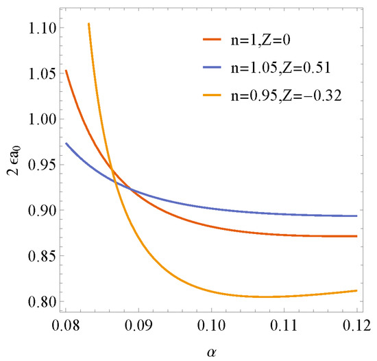
Figure 8.
Nonlinear threshold finite wave amplitude in the sub-critical unstable region for various n and Z with α at Re = 5.
Figure 9 shows how the nonlinear threshold amplitude at Re = 10 will be affected by different plane movement speeds and power-law index values while varies α from 0.03 to 0.07, which is in the supercritical stable region. The three curves are in different areas because the supercritical stable region for the three conditions corresponds to three different ranges of wave number α. The upward movement and the decrease in the power-law index cause the supercritical stable region to move to the larger wave number and the nonlinear threshold amplitude increase, and the film flow will become relatively more unstable. The downward movement and the increase in the power-law index cause the supercritical stable region to move to the smaller wave number and the nonlinear threshold amplitude decrease, and the film flow will become relatively more stable. The wave speed in Equation (45) is predicted to be a constant value for all wave numbers by using linear stability theory. The wave speed in Equation (55) is predicted to be a function of wave number α, Reynolds number, the power-law index n, and plane speed Z, by using nonlinear stability theory. Figure 10 shows how the nonlinear wave speeds at Re = 10 will be affected by different plane movement speeds and power-law index values while α varies from 0.03 to 0.07, which is in the supercritical stable region. The nonlinear wave speed increases as the upward movement increases and the power-law index decreases. It shows the stable condition becomes stricter as the upward movement and the power-law index decrease.
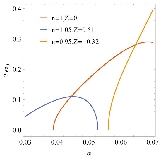
Figure 9.
Nonlinear threshold finite wave amplitude in the supercritical stable region for various n and Z with α at Re = 10.
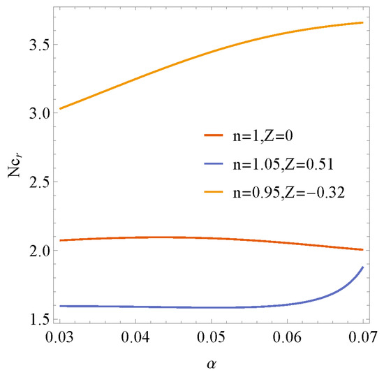
Figure 10.
Nonlinear wave speeds of the film flow in the supercritical stable region for various n and Z with α at Re = 10.
For each particular power-law flow and plane movement, this article builds a model to analyze the linear and nonlinear stability. By substituting different n and Z into the model, the Landau equation will show the state of the film flow, and the characterization of the stability can be revealed easily.
As discussed above, it becomes obvious that the characterization of film flow stability is significantly affected by the plane movement and power-law index. The effect of downward speed has the same tendency as the effect of the power-law index, but the specific behaviors are different.
If the power-law index is set to 1, the data can be compared with the results given by Lai et al. [8]. It is found that both sets of data agree well with each other.
4. Conclusions
The stability analysis of thin power-law fluid film flowing down a moving plane in a vertical direction is discussed in this article by applying the method of long-wave perturbation. It derived the generalized nonlinear kinematic equation of the power-law film on the free surface of the moving plane. The characterization of the flow stability has been analyzed. Based on the results above, several conclusions can be made:
- The neutral stability curve in the linear stability analysis is obviously affected by the movement of the plane and non-Newtonian fluid characteristics. The linear stable region increases as the downward speed increases and the power-law index increases. On the other hand, the linear stable region decreases as the upward speed increases and power-law index n decreases.
- By applying the Landau equation, the nonlinear neutral stability curve separates the flow field into four different regions: sub-critical instability, sub-critical stability, supercritical stability, and explosive supercritical instability. The regions of sub-critical instability and absolute stability are expanded when the plane’s downward speed increases or the power-law index increases, and meanwhile, the parts of supercritical stability and explosive supercritical instability are compressed. The parts of sub-critical instability and absolute stability are compressed when the plane’s upward speed increases or the power-law index decreases, and meanwhile, the parts of supercritical stability and explosive supercritical instability are expanded. Threshold amplitude in the sub-critical instability region and both the threshold amplitude and the nonlinear wave speed in the supercritical stability region show that the stable condition of the film flow is stricter than the same initial finite-amplitude disturbance when the upward speed increases and the power-law index decreases.
- The stability behavior of thin power-law fluid film flowing down a moving plane in a vertical direction is significantly affected by both the movement and the power-law index. The downward motion and larger value of the power-law index will tend to enhance the stability of the flow system.
- By substituting the power-law index n and moving speed Z into the generalized nonlinear kinematic equation of the power-law film on the free surface, the results can be used to estimate the stability of the thin film flow in oil paint, semiconductor manufacturing, pharmaceutical and chemical engineering, and other fields of applications.
Author Contributions
Conceptualization, C.-K.C. and W.-M.L.; methodology, C.-K.C.; software, W.-M.L.; validation, W.-M.L.; formal analysis, W.-M.L.; resources, W.-M.L.; data curation, W.-M.L.; writing—original draft preparation, W.-M.L.; writing—review and editing, W.-M.L.; visualization, W.-M.L.; supervision, C.-K.C. All authors have read and agreed to the published version of the manuscript.
Funding
This research was funded by the Ministry of Science and Technology of Taiwan, grant number MOST 109-2221-E-006-053-MY2.
Data Availability Statement
Not applicable.
Conflicts of Interest
The authors declare no conflict of interest.
References
- Lin, C.C. The Theory of Hydrodynamic Stability; Cambridge University Press: Cambridge, UK, 1955. [Google Scholar]
- Chandrasekhar, S. Hydrodynamic and Hydromagnetic Stability; Oxford University Press: Oxford, UK, 1961. [Google Scholar]
- Kapitza, P.L. Wave flow of thin viscous liquid films. Zh. Exper. Teor. Fiz. 1949, 18, 3–28. [Google Scholar]
- Benney, D.J. Long Waves on Liquid Films. J. Math. Phys. 1966, 45, 150–155. [Google Scholar] [CrossRef]
- Lin, S.P. Finite amplitude side-band stability of a viscous film. J. Fluid Mech. 1974, 63, 417–429. [Google Scholar] [CrossRef]
- Nakaya, C. Equilibrium states of periodic waves on the fluid film down a vertical wall. J. Phys. Soc. Jpn. 1974, 36, 921–926. [Google Scholar] [CrossRef]
- Krishna, M.V.G.; Lin, S.P. Nonlinear stability of a viscous film with respect to three-dimensional side-band disturbances. Phys. Fluids 1977, 20, 1039–1044. [Google Scholar] [CrossRef]
- Tsai, J.-S.; Hung, C.-I.; Chen, C.-K. Nonlinear hydromagnetic stability analysis of condensation film flow down a vertical plate. Acta Mech. 1996, 118, 197–212. [Google Scholar] [CrossRef]
- Lai, H.-Y.; Sung, H.-M.; Chen, C.-K. Nonlinear stability characterization of thin Newtonian film flows traveling down on a vertical moving plate. Commun. Nonlinear Sci. Numer. Simul. 2005, 10, 665–680. [Google Scholar] [CrossRef]
- Naganthran, K.; Hashim, I.; Nazar, R. Triple Solutions of Carreau Thin Film Flow with Thermocapillarity and Injection on an Unsteady Stretching Sheet. Energies 2020, 13, 3177. [Google Scholar] [CrossRef]
- Naganthran, K.; Hashim, I.; Nazar, R. Non-uniqueness solutions for the thin Carreau film flow and heat transfer over an unsteady stretching sheet. Int. Commun. Heat Mass Transf. 2020, 117, 104776. [Google Scholar] [CrossRef]
- Naganthran, K.; Nazar, R.; Siri, Z.; Hashim, I. Entropy Analysis and Melting Heat Transfer in the Carreau Thin Hybrid Nanofluid Film Flow. Mathematics 2021, 9, 3092. [Google Scholar] [CrossRef]
- Rehman, K.U.; Khan, A.A.; Malik, M.Y.; Makinde, O.D. Thermophysical aspects of stagnation point magnetonanofluid flow yields by an inclined stretching cylindrical surface: A non-Newtonian fluid model. J. Braz. Soc. Mech. Sci. Eng. 2017, 39, 3669–3682. [Google Scholar] [CrossRef]
- Rehman, K.U.; Malik, M.Y.; Mahmood, R.; Kousar, N.; Zehra, I. A potential alternative CFD simulation for steady Carreau–Bird law-based shear thickening model: Part-I. J. Braz. Soc. Mech. Sci. Eng. 2019, 41, 176. [Google Scholar] [CrossRef]
- Cheng, P.-J.; Chen, C.-K.; Lai, H.-Y. Nonlinear stability analysis of the thin pseudoplastic liquid film flowing down along a vertical wall. J. Appl. Phys. 2001, 89, 8238–8246. [Google Scholar] [CrossRef]
- Cheng, P.-J.; Lai, H.-Y.; Chen, C.-K. Stability analysis of thin viscoelastic liquid film flowing down on a vertical wall. J. Phys. D Appl. Phys. 2000, 33, 1674–1682. [Google Scholar] [CrossRef]
- Amaouche, M.; Djema, A.; Ait Abderrahmane, H. Film flow for power-law fluids: Modeling and linear stability. Eur. J. Mech. B/Fluids 2012, 34, 70–84. [Google Scholar] [CrossRef]
- Cheng, P.J.; Chen, C.K.; Wang, Y.C.; Lin, M.C.; Yang, C.K. Nonlinear Rupture of Thin Micropolar Liquid Film Under a Magnetic Field. J. Mech. 2016, 33, 249–256. [Google Scholar] [CrossRef]
- Lin, M.-C. Stability Analysis of a Thin Pseudoplastic Fluid with Condensation Effects Flowing on a Rotating Circular Disk. Adv. Mater. Res. 2013, 699, 413–421. [Google Scholar] [CrossRef]
- Chen, C.-I.; Chen, C.-K. Nonlinear stability analysis of the thin micropolar film falling exterior to a rotating vertical cylinder. Math. Model. 2005, 469, 168. [Google Scholar]
- Lin, M.-C.; Cheng, P.-J. Hydromagnetic Stability of a General Viscous Fluid Film With Weakly Nonlinear Effects on a Rotating Vertical Cylinder. J. Chin. Soc. Mech. Eng. 2021, 42, 33–41. [Google Scholar]
- Tomita, U. Rheology; Corona: Tokyo, Japan, 1964. [Google Scholar]
- Edwards, D.A.; Brenner, H.; Wasan, D.T. Interfacial Transport Processes and Rheology; Butterworth-Heinemann: Boston, MA, USA, 1991. [Google Scholar]
- Ginzburg, V.L.; Landau, L.D. Theory of superconductivity. J. Exp. Theor. Phys. 1950, 20, 1064–1082. [Google Scholar]
Publisher’s Note: MDPI stays neutral with regard to jurisdictional claims in published maps and institutional affiliations. |
© 2022 by the authors. Licensee MDPI, Basel, Switzerland. This article is an open access article distributed under the terms and conditions of the Creative Commons Attribution (CC BY) license (https://creativecommons.org/licenses/by/4.0/).