Abstract
Transport of cells in fluid flow plays a critical role in many physiological processes of the human body. Recent developments of in vitro techniques have enabled the understanding of cellular dynamics in laboratory conditions. However, it is challenging to obtain precise characteristics of cellular dynamics using experimental method alone, especially under in vivo conditions. This challenge motivates new developments of computational methods to provide complementary data that experimental techniques are not able to provide. Since there exists a large disparity in spatial and temporal scales in this problem, which requires a large number of cells to be simulated, it is highly desirable to develop an efficient numerical method for the interaction of cells and fluid flows. In this work, a new Fluid-Structure Interaction formulation is proposed based on the use of hybrid continuum-particle approach, which can resolve local dynamics of cells while providing large-scale flow patterns in the vascular vessel. Here, the Dissipative Particle Dynamics (DPD) model for the cellular membrane is used in conjunction with the Immersed Boundary Method (IBM) for the fluid plasma. Our results show that the new formulation is highly efficient in computing the deformation of cells within fluid flow while satisfying the incompressibility constraints of the fluid. We demonstrate that it is possible to couple the DPD with the IBM to simulate the complex dynamics of Red Blood Cells (RBC) such as parachuting. Our key observation is that the proposed coupling enables the simulation of RBC dynamics in realistic arterioles while ensuring the incompressibility constraint for fluid plasma. Therefore, the proposed method allows an accurate estimation of fluid shear stresses on the surface of simulated RBC. Our results suggest that this hybrid methodology can be extended for a variety of cells in physiological conditions.
1. Introduction
Dynamics of biological cells in fluid flows are important in many areas of bio-engineering [1]. The transport of cells in the human body is the main mechanism to sustain life as it provides oxygen, nutrient, and defensive mechanism to fence off infection. Human cells are comprised of many compartments such as bi-lipid membrane, cytoplasm, nucleus, and others [2]. However, special cells such as the Red Blood Cell (RBC), White Blood Cell (WBC), and platelet, are contained mostly of a thin membrane and cytosol fluid [3]. RBC, WBC, and platelet [4] are the main components of human blood. Therefore, understanding their dynamics could lead to new innovations in many engineering areas such as biomedical devices [5,6], cancer biology [7,8], or drug delivery [9]. From a mechanical standpoint, these special cells (or capsules) are deformable bodies, which are immersed in a flowing fluid. Investigating the dynamics of these cells can be useful for many engineering applications such as the detection of malaria infection [10], cell sorting/separation [11], drug delivery [12], and design of devices for blood fractionation [13]. Modeling the dynamics of these special cells in fluid flow is the focus of the current work.
While many aspects of cellular flows can be examined by in-vitro experiment [14] in well-controlled conditions, it is challenging to replicate all physiological conditions in the laboratory. In the last decade, numerical simulations have shown promises [15] in investigating transport of cells in realistic anatomy of vascular systems [2]. The growth of computing power has enabled the simulation of whole blood, which consists of RBC, WBC, and platelet interacting with each other [16]. The central challenge here is the multi-way interactions of these capsules with the fluid flow and with each other. In addition, the complex anatomy of the vascular system is a great challenge for computational methods to deal with [17] since cells migrate along the bifurcations without a predetermined pattern. Here, numerical methods must be able to resolve the local dynamics of cells as well as provide sufficient details of large scale flows in the vascular vessels. This task motivates a variety of approaches as listed below.
In a single cell, Molecular Dynamics (MD) [18,19] simulation is the method of choice for calculating cellular membrane dynamics since it can provide a good estimation of lipid bilayer dynamics. However, MD requires a large number of particles (few millions) to mimic the behavior of the membrane [19,20,21]. This approach is thus not appropriate for a large-scale simulation of multiple cells.
Continuum approach such as the Finite Element method [16,17,22,23] and boundary integral methods [24,25,26] have been used to describe the dynamics of RBC membrane. These continuum approaches require solving the non-linear systems of equations to calculate the finite deformation of the cell membrane. Currently, simulations using these methods have reported the dynamics of a few hundred of thousands RBCs [16,22,23], which are still far from physiological values in the arterial system.
The need to develop an efficient method for the cellular membrane has led to the emergent use of Dissipative Particle Dynamics (DPD) [27] in cellular flows. Pivkin et al. [20] and Fedosov et al. [21] proposed the state-of-the-art coarse-grained RBC model based on the Dissipative Particle Dynamics approach. Following this method, only a few hundred particles are required to simulate RBC dynamics. Therefore, the computational cost is reduced significantly. In this approach, both the fluid plasma and cellular membrane, and the cytoplasm are simulated with the DPD method. To date, this coarse-grained DPD modeling has enabled a series of investigation of Red Blood Cell, White Blood Cell, and platelet in idealized models of vasculatures [15,28]. This DPD method is successful in simulating many behaviors of cells such as tank-treading and tumbling [29], deforming through a slit [25,30], or moving through stenosis collapse [31], or micro-fluidic devices [32]. However, the difficulty in resolving the interaction between fluid plasma and cell membrane remains a great challenge for DPD methods [15] since it is not clear how to assign physical values to DPD models of the fluid. As a particle-based method, the advantage of the DPD method is the flexibility in modeling complex fluids as the method satisfies conservation laws and other related constitutive equations [15]. However, there is a number of disadvantages for the DPD method such as the uncertain mechanism to set the physical values for governing parameters such as viscosity, density, and others. The DPD method only approximates fluid dynamics in the averaging sense (e.g., mean density and mean momentum). Therefore, it is challenging to apply the scaling arguments to the equations of motion for the DPD method. It is thus important to come up with a new method for simulating the fluid plasma separately from the RBC cytoskeleton dynamics.
Recognizing the challenges in coupling dynamics of cellular membranes and the fluid plasma, many numerical methods have been proposed to use different models for fluid plasma and the cell membrane [33] via the use of the immersed boundary method. In this type of coupling, fluid plasma can be described separately from the cell membrane model. For example, the Lattice Boltzmann Immersed Boundary method has also been developed [31,34,35]. In this model, the Lattice Boltzmann Method (LBM) [2], a particle-based method, is used to simulate the fluid plasma while the DPD or Finite Element model is used for the cell membrane. Other numerical methods for fluids have been proposed as well such as the Finite Element Method [36] or Finite Difference methods [17]. Particular roadblocks for this type of fluid-cell interaction coupling are: (a) High computational cost to simulate individual cell dynamics; (b) incompressibility constraint of the fluid plasma; and (c) enforcing a no-slip boundary condition of fluid flow in anatomical geometries of the arterial vasculature. These difficulties have been addressed separately in recent attempts [17,28,31] for a small domain. However, these are still major challenges if it is required to evaluate the hemodynamics of a significantly large portion of the arterial tree such as the coronary arteries [22]. It is highly desired to devise a numerical strategy so that these roadblocks are removed with ease.
In this work, we propose a new approach based on the concept of continuum-particle coupling. The cell membrane is modeled using the coarse-grained particle approach (DPD) while the fluid plasma is simulated using the continuum approach (sharp-interface IBM). The coupling of dynamics between the cell membrane and the fluid plasma is carried out using Fluid-Structure Interaction (FSI) methodology. Such a combination allows the incompressibility of fluid plasma is satisfied while accommodating the FSI simulation of cells in anatomical geometries.
Our manuscript is organized as follows. Firstly, we describe the essential components of the immersed boundary method for incompressible fluids in Section 2.1. Secondly, the DPD methodology to simulate the dynamics of the lipid bi-layer membrane is explained in Section 2.2. Thirdly, the FSI methodology between the membrane and the fluid plasma is discussed in Section 2.3. Finally, several numerical examples are investigated to examine the ability of the proposed framework for simulating RBC dynamics in different fluid flows in Section 3. Discussions on the advantages and disadvantages of the proposed method will be shown in Section 4 and Section 5.
2. Materials and Methods
2.1. Mathematical Descriptions of the Cell-Fluid Interaction Using the Sharp-Interface Immersed Boundary Method
The cell (erythrocyte) is considered as a body , which is immersed in a fluid (blood plasma). The surface of the cell () is represented by a triangulated network [37]. The computational mesh for the fluid domain is therefore separated into two parts: (a) The outer part (blood plasma) and (b) the inner part as shown in Figure 1.
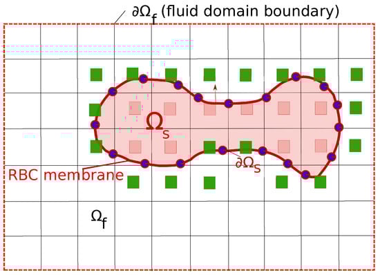
Figure 1.
The representation of the Red Blood Cells (RBC) inside the fluid plasma using the Immersed Boundary Method (IBM). The RBC membrane is the surface of the solid domain (), which is depicted as a line connected by blue circles. The fluid domain is denoted as with the appropriate boundary conditions . The green squares represent the immersed nodes, which are the adjacent nodes to the cell surface . The no-slip boundary condition is enforced on .
The dynamics of the cell is modeled via a Fluid-Structure Interaction (FSI) procedure since the cell deformation is under the impacts of the fluid forces and vice versa. Thus the cell and fluid motions are tracked simultaneously. On , the no-slip boundary condition and the continuity of stresses are enforced. For the details of the coupling, the interested reader is referred to our previous publications [37,38]. Only essential components of the FSI methodology is discussed here.
The governing equations for the fluid motion in is the Navier–Stokes equations. The Curvilinear Immersed Boundary method (CURVIB) [39] is used to solve the govering equation in curvilinear computational mesh. CURVIB uses the hybrid staggered/non-staggered approach [40] to solve the Navier–Stokes equations. Three-point central differencing are carried out for all spatial derivatives. Time integration is done via a second-order accurate fractional step method. The momentum equation are solved with a Jacobian-free solver while Flexible Generalized Minimal Residual () method with a multigrid pre-conditioner used to solve the Poisson equation to satisfy the discrete continuity equation to the machine-zero precision. Complex solid boundaries such as the membrane surface are handled using the sharp-interface IBM with the velocity reconstruction along the local normal to the body [41] as shown in Figure 1. In this approach, the presence of a RBC in the fluid domain is substituted by the immersed nodes where the velocity reconstruction is carried out so that the no-slip boundary condition is satisfied on (green squares in Figure 1). The procedure to solve the fluid equations is denoted as the fluid solver .
The CURVIB method is now implemented in the Virtual Flow Simulator (VFS), which is an open-source code released on 10 April 2015 and can be downloaded at http://safl-cfd-lab.github.io/VFS-Wind/, accessed on 1 February 2021. VFS has been applied for many problems in biological applications including brain aneurysms [42,43], heart hemodynamics [44,45,46], and heart valves [47,48].
2.2. Membrane Modeling
The RBC membrane is assumed to consist of a lipid bilayer attached to an inner cytoskeleton, which is a structure comprised by spectrin proteins and actins in a compact network. The cell’s physical characteristics, such as the viscosity, the elasticity, and the bending stiffness, are derived fundamentally from these biological components. To mimic the interconnected structure of the cytoskeleton, the RBC membrane is modeled as a spring-network structure (a triangular mesh on a 2D surface), as described in [20,21]. Here, we follow the Dissipative Particle Dynamics approach [20,21,49] to simulate the dynamics of this network. The details of the computational methodology are as follows.
2.2.1. Red Blood Cell Geometry and Network Triangulation
The shape of a normal RBC can be described using an analytical function [20]. The average shape of a RBC membrane [20,21] is given by a set of points with coordinates in space:
The parameters are chosen as m (cell diameter), , , and . The area and volume of this RBC are equal to 135 (m) and 94 (m), respectively (see also Table 1).

Table 1.
Dissipative Particle Dynamics (DPD) parameters for the model of RBC membrane for different number vertices . is the model length scale, is the equilibrium length of the links, is the maximum length of the links, p is the persistence length, and is the spontaneous angle. In these cases, , , , m, and m, respectively. Other parameters are , Ns/m, and .
As the surface is known precisely according to Equation (1), the triangulation procedure is carried out to mimic the distribution of the spectrin links on the membrane [20]. Using an open-source code distmeshsurface [50], the surface is triangulated with a predefined number of vertices . The robustness of distmeshsurface allows it to generate a high-quality triangular mesh precisely on a 3D surface using a signed distance function.
2.2.2. Modeling the RBC Membrane Using the Spectrin-Link Method
The membrane model is described by a two-dimensional triangulated network on a three-dimensional membrane surface as shown in Figure 2a. The network is composed by a collection of points with its Cartesian coordinates in Figure 2b. Here the index indicates the vertex of the surface triangulation. The vertices are connected in pairs by springs (edges between the vertex i and j) forming number of triangles.
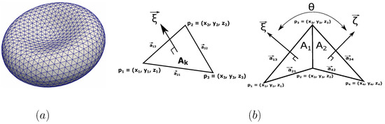
Figure 2.
(a) Triangulated surface of the spectrin network attached to the lipid bilayer membrane. The numbers of vertices and triangles are denoted as and . The number of vertices varies from to points (nodes). (b) The definition of the normal surface vector and the spontaneous angle between two adjacent elements. A element is defined by three vertices of the triangulated network.
All the equations presented in this work, describing the DPD model are taking directly from the work done by Pivkin et al. [20] and Fedosov et al. [21].
The internal forces () is related to the Helmholtz’s free energy V as:
Here is the position vector of the vertices.
The potential energy of the system includes the in-plane, bending, and area/volume constraints:
The in-plane free energy term includes the elastic energy stored in the membrane. Here, the nonlinear wormlike-power model [20] is used:
The Wormlike Chain (WLC) attractive potentials () for individual links is expressed as:
where is the length of the spring j, and represents the spring deformation. and p are the maximum length of the links and the persistence length, respectively. and T are the Boltzmann’s constant and the temperature, respectively.
The energy potential, [21], which defines a repulsive force in the form of a power function . depends on the separation distance as:
where is the force coefficient and m is the exponent.
The bending energy is defined as,
Here and are the bending constant and the spontaneous angle, respectively. is the instantaneous angle between two adjacent triangles, which share the common edge (link) j as seen in Figure 2b.
The area and volume conservation constraints account for the incompressibility of the lipid bilayer and the inner cytosol, respectively. They are defined as:
Here, and is the instantaneous area of the triangle (element) and the average area per element. , , and are the global area, local area, and volume constraint coefficients, respectively. A and V are the instantaneous total area and total volume of the RBC. The and are the specified total area and volume, respectively. The procedure to evaluate the values of and is carried out from individual elements as shown in Figure 2b [51]. In each triangle (element) of the network, three sides are established by linking the respective vertices 1, 2, and 3 as seen in Figure 2b. The length of the side connecting two vertices i and j (1, 2, or 3) can be computed as . Here is the vector position of the vertex i or j (). The normal vector of the element can be derived from the cross product of and as shown in Figure 2b. Note that the area and volume of a single triangle element can be also calculated from as and . Here is the position vector of the triangle centroid.
Finally, the internal force contribution from vertex can be computed from Equation (2) as:
2.2.3. Membrane Viscosity
The RBC membrane is viscoelastic in nature. The membrane viscosity contribution is expressed as an additionally dissipative force as [51],
where and are dissipative paramaters. Here the relative velocity between two adjacent vertices in the same link (i and j) is . The position vector of the link is . The membrane viscosity is a function of both dissipative paramaters, and . Here is responsible for a large portion of the membrane viscosity in comparison to . Following the suggestion of Fedosov et al. [51], is set to be equal to one third of . Consequently, these parameters relate to the physical viscosity of the membrane as:
So, the dissipative force of the membrane is:
2.2.4. Coarse-Graining Procedure
A full-scale model of a RBC typically consists of millions of particles [19], which are required to accurately simulate protein dynamics. However, it is not feasible to use such a full-scale model in a FSI simulation due to the computational cost. In this work, we follow the coarse-graining procedure of Pivkin et al. [20] to represent the RBC membrane by a smaller number of particles (vertices). This procedure does not allow a detailed simulation of separate proteins but it is versatile enough to capture the overall dynamics of the RBC membrane.
Based on the equilibrium condition, Pivkin et al. [20] proposes a coarse-graining procedure based on the area/volume constraint for the spring equilibrium () and maximum () lengths as follows:
where the subscript c and f refer to the coarse-grained and the fine models, respectively.
Note that the role of is critical in determining the response from the WLC model as seen in Equation (5). From the numerical standpoint, the RBC membrane model is highly sensitive with the value of and .
As the number of vertices reduces, the average angle between the pairs of adjacent triangles increases. The spontaneous angle is adjusted in the coarse-grained model as [52]:
Due to the scaling in Equation (12), the value of does not change as the model is coarse-grained. To maintain the shear and area-compression moduli, the parameters p and are adjusted as [21]:
2.2.5. Scaling of Model and Physical Units
One challenge in DPD modeling [28] is the relationship between the modeled quantities and the physical values since this relationship is not explicit. It is necessary to use a scaling argument to recover this relationship [21,29]. Here, the superscript M and P corresponds to the model and physical units (SI units), respectively.
The length scale () is defined as:
is the model unit of length. To be explicit, is the cell diameter in the model unit and is the physical cell diameter in meters.
The energy per unit mass() and the force N scaling values are given by:
with Y is the membrane Young’s modulus. The timescale is defined as following:
Here is the membrane viscosity.
2.2.6. Time-Integration Scheme for the DPD Model
The motion of each vertex i can be , which is described by the Newton’s second law of motion:
where , are the position and velocity of the vertex i, respectively. The mass per vertice is defined as the mass per vertex . The internal forces is computed from Equation (9). Using the previous scaling methodology in Section 2.2.5, the total mass of the RBC in the DPD model is set to be . Since the time scale is sufficiently small, we use the explicit Euler method to integrate Equation (18) in time. The timestep is chosen to be compatible with the DPD time scale as explained further in Section 3.
The external forces result from the fluid motion acting on the membrane. Therefore the traction vector on must be evaluated from the fluid stress tensor as . The normal vector of the surface at vertex i is . The details of evaluation has been explained in our previous work [37] extensively. In our method, the is computed directly from the fluid velocity and pressure field in the vicinity of the membrane. Note that the fluid velocity and pressure field are the solutions of the Navier–Stokes equations in the domain . In brief, the external forces are evaluated as:
Here is the nodal area, which is the assigned area of vertex i.
2.3. Fluid Structure Interaction Methodology for Cellular Structures
The cellular structure () of Section 2.2 is developed to simulate the membrane deformation in fluid flow. A FSI procedure is developed to link the dynamics of the cellular membrane with the fluid plasma using the immersed boundary method as described in Section 2.1. The details of the FSI procedure has been developed and reported in our previous works [38]. To facilitate the discussion, we describe only the relevant aspects of our computational methodology as follows.
The deformable body (RBC-) is immersed in the fluid plasma as shown in Figure 1. The RBC membrane described in Section 2.2 is the interface between and : . The solid domain deforms under the impacts of the fluid stresses. Our FSI algorithm is to determine the deformation of .
Here the fluid plasma () is considered as a Newtonian incompressible fluid. The incompressible Navier–Stokes equations in Section 2.1 are used to model the dynamics of the fluid plasma. The deformation of the solid body is governed by the DPD model as described in Section 2.2. On the one hand, the deformation of the RBC () is transferred to the flow field via the velocity field (Dirichlet boundary). On the other hand, the fluid stresses and associated traction vector (Neumman boundary condition) are transferred from the fluid domain to the solid domain. The displacement field of the particles (vertices) can be found via a fixed-point iteration (refer to [53] for example):
Here is the short-hand notation to describe the governing equations of the fluid domain while denotes the governing equations of the solid domain. The operator ∘ represents the load and displacement continuity conditions that are enforced on the interface . Since this non-linear equation is typically stiff, different methods have been proposed to solve Equation (20) effectively. In the current work, fixed point iteration with relaxation (Aitken’s acceleration) [41] is used to solve Equation (20) for a time step from a known solution at time step n.
3. Results
The dynamics of RBCs are investigated under different conditions: (a) Dynamic stretching under a pulling force; (b) relaxing in a uniform flow; (c) deforming under shear flow in a confined tube; and (d) moving through a curved tube. These tests will demonstrate the capability of the FSI methodology in modeling the interaction of a RBC with fluid flows.
3.1. Dynamics of RBC under Stretching
Mills et al. [14] studied the deformation of a single Red Blood Cell under stretching with optical tweezers. The RBC is attached to two silica microbeads (d = 4.12 m) in a solution of Phosphate-Buffered Saline and Bovine Serum Albumin. Cell stretching is carried out by holding one microbead fixed while moving the other one with force F. For each stretching test, the axial diameter () and transverse diameter () are measured with the corresponding value of F. Here, the axial diameter is defined along the direction of stretch. The transverse diameter is measured in the orthogonal direction to the stretch direction. The definitions of and are shown in Figure 3. The experimental results of Mills et al. [14] are shown in Figure 4 with the error bounds indicating a significant variations of the value.
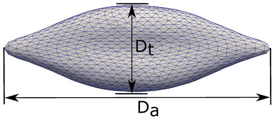
Figure 3.
Definitions of the axial diameter () and the traverse direction (). The deformation of the RBC is measured by the quantities and as shown in Figure 4.
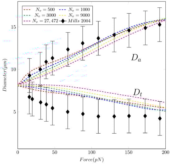
Figure 4.
The evolution of the axial and transverse diameters ( and ) of the RBC versus stretching force F. The experimental data from [14] is shown with a black line with error bounds. The coarse-graining simulations are shown with lines: Red (), blue (), green (), yellow (), and magenta ().
To validate our RBC model, we perform the simulation of the stretching test of Mills et al. [14] following the suggestion of Pivkin et al. [20]. In our simulation, the applied force F locates axially from both sides within the contact area of the microbeads. In our simulation, the magnitude of the force F is incrementally increased from 0 to 200 in a step-wise manner (quasi-static) with a number of 16 steps in the total stretching period. The force is kept constant within each step so that the cell membrane has sufficient time to relax to a constant value. We perform our simulations with different values of vertices and . The detailed values for each simulation are reported in Table 1.
Our results in Figure 4 and Figure 5 show that the model replicates the RBC membrane dynamics reasonably well for different stretching forces. The value of in the proposed model agrees well with experimental data. However, the simulations underpredict the values of across different . Nevertheless, the simulated values of are still in the upperbound of experimental values. Examining the shapes of the RBC under different values of F shows that the proposed model provide a consistent RBC shape across different values of vertices number . As the stretching force is increased from 0 to 150 , the maximum length () and the minimum length () varies in a similar fashion of previous studies, both computations [20,21] and experiment [14]. Therefore, the robustness of the coarse-graining procedure has been demonstrated successfully. With only vertices, the RBC membrane deformation shows a consistent behavior even in cases with much higher values of . Unlike the continuum approaches, the DPD method is known to be insensitive to mesh refinement [20,21]. Therefore, choosing the appropriate value of must balance between the computational cost and required dynamics to be captured. Therefore, it is sufficient and economical to use the DPD model with to represent the dynamics of RBC membrane as described below.
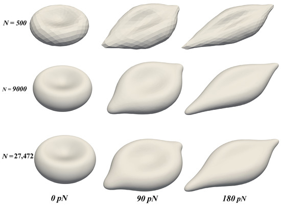
Figure 5.
The deformation of the RBC membrane under the stretching force F with different values of : 500 (top row), 9000 (middle row), and 27,472 (bottom row). Three time instants (see Figure 3) are chosen to demonstrate the dynamics: 0 pN (left column), 90 pN (middle column), and 180 pN (right column).
3.2. RBC Deformation in a Uniform Flow (No Shear)
Since the DPD model represents well the RBC dynamics under stretching as seen in Section 3.1, it is reasonable to apply it into the FSI simulation. As a first step, FSI simulations are performed to test the sensitivity of the FSI methodology under zero shear stresses condition.
The RBC is positioned at the center of a computational domain, which is a rectangular domain of size m and m as shown in Figure 6. The computational domain is discretized with a uniform structured mesh with different grid sizes: (a) Grid-1; (b) Grid-2; and (c) Grid-3 ranging from thousand to 1.5 million grid points as shown in Table 2. Since the coarse-grained DPD model represents well the dynamics of the RBC membrane as discussed in Section 3.1, it is used in this case. It is important to note that the spatial resolution of the structured mesh () must be able to resolve the RBC thickness. In addition, the spatial resolution of the triangular (unstructured) mesh of the RBC membrane should match the fluid mesh due to the requirement of the immersed boundary method. A uniform profile and the fully develop flow conditions are set at the inlet and outlet, respectively. Symmetry boundary conditions are set on other side planes.
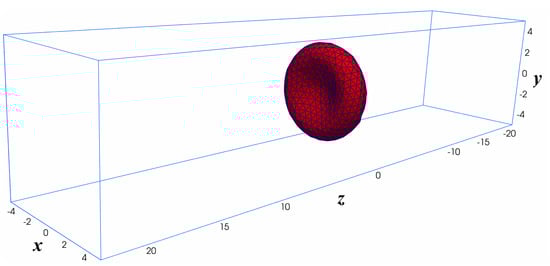
Figure 6.
Computational setup for the Fluid-Structure Interaction simulation of a single RBC in uniform flow. The computational domain is a structured mesh of size 10 m × 10 m × 45 m. The uniform flow (no shear) is applied at the (x-y) plane of m. The Neumman boundary condition is applied at the outlet. Symmetry (slip) boundary condition is applied on the other sides. The RBC is initially placed at the center of the computational domain .
Table 2.
Grid refinement study for the Fluid-Structure Interaction (FSI) simulation of a single RBC in uniform flow. The RBC is simulated with the coarsest DPD model () as seen in Table 1. The domain (−5:5, −5:5, −22.5:22.5) m is discretized as a structured grid with uniform spacing in directions as shown in Figure 6.
First, the uniform inflow is linearly increased from 0 to a maximum velocity of mm/s at the inlet within 20 s. After that, the uniform flow profile with is kept constant with time. Using the length scale of the cell diameter m and the fluid viscosity of m/s, the maximum Reynolds number of the fluid domain is calculated as . In this case, the time scale of the DPD method (particles) is governed by Equation (17). This time scale is smaller than the one required by the immersed boundary method. Therefore, the DPD time scale ( microsecond) is adopted in this work. Since the flow is uniform at a very low Reynolds number, it is expected that the RBC deforms minimally and mostly propagates along the flow direction.
The dynamics of the RBC under the gradually increased load of the incoming flow at different time instances is shown in Figure 7. Initially, the shape of the RBC is set to be the analytical shape as discussed in Section 2.2 at as shown in Figure 7A. However, the RBC starts to relax toward the stress-free condition as shown in Figure 7B,C after 400 s. As the RBC shape reaches its equilibrium condition, it translate along the flow direction (x).
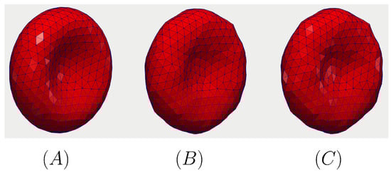
Figure 7.
The relaxation of the RBC under zero-shear condition. The initial shape of the RBC is the analytical shape as discussed in Section 2.2 at (A). The RBC relaxes toward the stress-free condition in (B) ( s) and (C) ( s). The results are taken from the Grid-1 simulation as indicated in Table 2.
The results of the grid refinement study are shown in Figure 8. The shape of the simulated RBC is compared across different sizes of the fluid mesh (see Table 2) on the x symmetry plane at s. It is shown that the RBC shapes agree well with each other. Therefore, the proposed numerical method for FSI simulation of RBC is consistent.
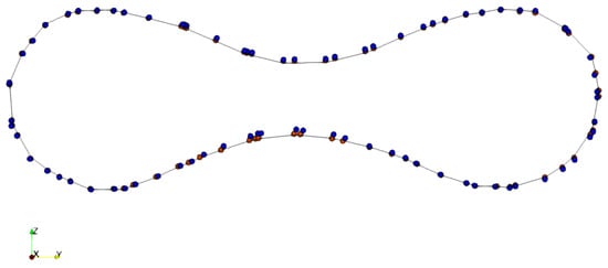
Figure 8.
The impacts of computational mesh size on the simulated results of RBC deformation. The shape of the RBC membrane is shown in a symmetry plane orthogonal to the x direction at the time instance of 240 s. The position of the vertices of the RBC in Grid-1, Grid-2, and Grid-3 (see Table 2) are shown in blue points, red points, and the solid line, respectively. The shape of the RBC is nearly identical under different computational grids.
3.3. Fluid-Structure Interaction Simulation of an Immersed RBC in a Confined Tube
To illustrate the capabilities and robustness of the proposed model under shear flow, we replicate the simulation procedure proposed by Pivkin et al. [20]. The computational domain resembles the Poiseuille flow with the tube diameter of m as shown in Figure 9. The RBC is initially placed at the center of the domain. Here we also use the coarse-grained DPD model with as discussed in Table 1.
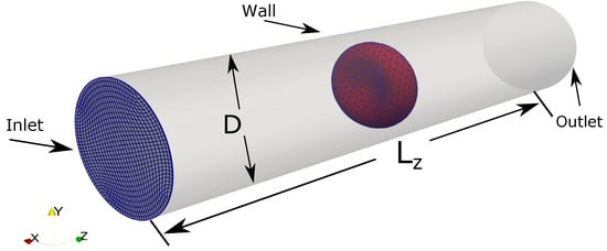
Figure 9.
The computational setup for the Fluid-Structure Interaction simulation between a single RBC in a Poiseuille flow. The computational domain (the tube) is a structured mesh of size with the average spacing in directions are approximately 0.4 m × 0.4 m × 0.9 m. The curvilinear mesh at the plane is shown in blue for an illustration of the computational mesh. Time-varied uniform flow is prescribed at the inlet at . The fully developed boundary is applied at the outlet. Wall boundary (no-slip) condition is applied on the tube wall. The diameter of the tube and its length are m and m, respectively. The RBC model () is initially placed at the center of the domain.
A time-varied uniform inflow profile is prescribed at the inlet . The value of is linearly increased from 0 to a maximum velocity of mm/s at the inlet within 20 s. After that, the uniform flow profile with is kept constant with time. Using the length scale of the pipe diameter m and the fluid viscosity of m/s, the bulk Reynolds number of the problem is . At the outlet, the Neumman boundary condition is applied. On the pipe wall, no-slip condition is enforced.
As the pressure gradient develops inside the tube, the RBC starts to deform as shown in Figure 10a (top row). Initially, it has a biconcave shape as discussed in Section 2.2. However, its transitions from the initial biconcave shape to a parachute shape within 1 ms. The transition is remarkable given that one side of the RBC membrane is pulled forward significantly. After this transition, the RBC propagates along the tube axis with minimal changes in its shape. Note that this phenomenon is widely observed in in-vitro experiments [54] and discussed extensively in literature [17,51]. During this process, the flow field inside the tube resembles closely the parabolic profile, except in the vicinity of the RBC membrane as illustrated in Figure 10b (bottom row). In brief, the FSI methodology accurately predicts the shape transition of the RBC in Poiseuille flow.

Figure 10.
The transition of the RBC shape from the biconcave shape into the parachute shape in the Poiseuille flow in Figure 9. The shape of the RBCs at , , and milliseconds are shown in (a) (first row). The corresponding flow fields are visualized using velocity contour and in-plane streamlines on one symmetry plane (b) (second row).
To examine the potential impacts of the triangular mesh resolution, two additional simulations are carried out with and as shown in Figure 11. Comparing between the case of and in Figure 11a,b, it is shown that the transition to the parachute shape is delayed in . The membrane seems to become stiffer with the larger value of . However, the differences of the RBC dynamics between the cases and are minimal. The RBC shapes for the refined cases ( and ) are nearly identical as depicted in Figure 11b,c. These results indicate that it is required that at least to reflect the RBC dynamics in micro-vessels accurately.
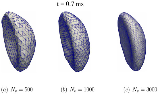
Figure 11.
The impact of DPD particles on the membrane dynamics during the fluid-structure interaction simulation. Three values of are examined: (a) , (b) , and (c) . The computational setup is shown and discussed in Figure 9, the fluid domain is chosen as Grid-1 (see also Table 2). In all cases, the simulated RBC is compared across different at the time instant t = 0.7 ms. The RBC is transitioning to the parachute shape. The RBC shape is nearly identical between and cases.
3.4. RBC Migration in an Artery Model
To illustrate the capability of the proposed method for flows in micro-vasculature, FSI simulation of a RBC in a curved tube is carried out as shown in Figure 12. The fluid domain is created as a curved tube of 12 m in diameter with arbitrary curvature. The tube (computational domain) is discretized with a structured grid of size with the approximate spacing 0.2 m × 0.17 m × 0.54 m in the directions, respectively. The RBC model () is initially placed at a distance of 20 m from the inlet.
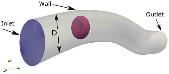
Figure 12.
The computational setup for the Fluid-Structure Interaction simulation between a single RBC and the flow in a curved tube, which is a model of a human arteriole. The tube is discretized as a structured grid of size with the approximate spacing 0.2 m × 0.17 m × 0.54 m in directions, respectively. The RBC model () is initially placed at a distance of 20 m from the inlet.
Similar to the previous cases, a time-varied uniform inflow profile is prescribed at the inlet . The value of is linearly increased from 0 to a maximum velocity of = 2 mm/s at the inlet within 20 s. After that, the uniform flow profile with is kept constant with time. Using the length scale of the pipe diameter D = 12 m and the fluid viscosity of m/s, the bulk Reynolds number of the problem is . At the outlet, the Neumman boundary condition is applied. On the tube wall, no-slip condition is enforced. The RBC starts to deform as shown in Figure 13, following the same deformation patterns in the previous case of a straight tube. One side of the cell is pulled strongly to achieve the parachute shape in almost the same time window of 1 ms. However, the shape of the RBC is not completely symmetric as one in a straight tube. Here, the tube curvature slightly impacts the deformation so that the RBC shape depends on the local curvature of the tube. In brief, the DPD model is able to respond to the local features of the complex flow in micro-channel geometries.
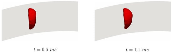
Figure 13.
Deformation of the RBC from the biconcave shape into the parachute shape in a curved tube. The shape of the RBC is shown at t = 0.6 and 1.1 milliseconds. The tube boundary is shown in the shadow.
4. Discussions
To our knowledge, the coupling of a continuum approach, such as the Immersed Boundary Method, and the particles systems of Dissipative Particle Dynamics, has never been carried out before. The novelty of our approach leads to several numerical advantages: (i) Satisfying the no-slip boundary condition on the cell surface; (ii) ensuring the incompressibility of the fluid plasma; and (iii) being flexible in handling anatomical geometries. The details of such advantages are explained below.
Due to the sharp-interface nature of the approach, the no-slip boundary condition on the cell surface can be satisfied easily. The sharp-interface immersed boundary method [40] ensures that the velocity in the closest fluid point (immersed nodes—see Figure 1) is reconstructed by interpolating between the flow field and the motion of the membrane surface. In our approach, the Navier–Stokes equations are the governing equations for fluid plasma. Hence, the incompressibility constraint is satisfied exactly for the fluid domain, which is not possible if particle-based methods such as LBM or DPD are used [33]. This incompressibility condition is important since it ensures an accurate estimation of the fluid shear stresses. Moreover, the use of an immersed boundary method simplifies the procedure to incorporate anatomical geometries of the arteries in our future works. This feature will be useful in simulating blood flow in arterioles and veins. In brief, our proposed method improves the accuracy of RBC dynamics simulations without increasing the computational cost significantly.
The state-of-the-art numerical methods for cellular flows are currently limited by the computational expense of resolving individual RBC dynamics (e.g., few hundred of thousands cells) [16,22,23]. Therefore, a computationally expedient algorithm will enable the simulation of cellular dynamics under physiological conditions. The use of DPD for RBC dynamics has been popularized [20,21] because the lipid bilayer and cytoskeleton mechanics can be described easily using a set of particles, which represents the cytoskeletal structure. Our results in Section 3.1 show that DPD is efficient and robust in simulating RBC deformation under a large range of impacting forces. This is remarkable given that the DPD model is much simpler in comparison to elaborated methods such as FEM [17,36]. With only particles, our results show that the DPD model yields cellular deformation in good agreement with previous computational and experimental data [14,17,20,21,55]. All simulations were performed with a relatively inexpensive computational cost. The computational cost of the DPD is negligible in comparison to the fluid flow solver using the immersed boundary method. Overall, each simulation requires 20 CPUs and 20 Gb RAM to run in approximately 24 h wall clock time.
We follow the original DPD model of Pivkin et al. [20]. In this model, the mass of RBC is set to be kg according to the force and length scales proposed by Pivkin et al. [20]. However, the real mass of one RBC varies from kg [56]. So, there is a significant difference in the modeled and real mass of the RBC. Our future work will investigate the dependence of the stability condition on the RBC mass.
The immersed boundary method has been used to simulate the dynamics of RBC in fluid flow in previous works [17,57] mostly in the context of diffuse interface. The membrane/fluid interface is typically tracked via a level-set approach [17], which ensures the continuity of viscosity distribution [23]. This diffusive interface approach does not allow a sharp distinction (or jump condition) of fluid properties from the inner and outer parts of the cell. Our approach allows the further development of a more complex model for RBC [19] since the RBC model is completely independent on the fluid model. Past works have ignored the dynamics role of cytosol [20]. Our approach can be easily extended to include this effect by developing a separate model for the cytosol. Furthermore, many other processes have not been considered in the current model such as the cell-cell interaction [31] and the cell-vascular wall interaction [2]. Our future efforts will further extend the framework to include such aspects.
In brief, our proposed method has several limitations. Firstly, it is challenging for the DPD method to set the important physical parameters such as the viscosity and the density of the RBC membrane independently. Secondly, the implementation of the immersed boundary method requires the continuous tracking of the RBC surface. In the current work, there is only one RBC that is simulated so the computational cost is negligible. However, a physiological condition in human arterioles might include millions of RBCs. Therefore, a special algorithm to accommodate such a tracking should be developed in future. Thirdly, the interaction between RBCs and the arterial wall must be simulated in a realistic condition. Therefore, a model for the collisions between the cells and vascular walls should be developed. Our future work will explore the use of the Morse Potential [30,31] to achieve this end.
5. Conclusions
In this work, we developed a new coupling approach between the sharp-interface IBM and the DPD to simulate the dynamics of cells in fluid flows. This hybrid continuum-particle method is then applied to simulate the transport of RBC in straight and curved tubes. Our results showed good agreements with experimental measurements as well as other computational works. Our results show that the new formulation is highly efficient in computing the deformation of cells within fluid flow while satisfying the incompressibility constraints of the fluid locally. This feature is critical for an estimation of fluid shear stresses on the surface of RBC as well as the vascular walls. Therefore, our proposed approach can be applied for many biomedical applications such as estimating the fluctuations of RBC membrane [19], thrombus formation, and blood clots [30,31]. Our results also suggest that this hybrid methodology can be extended for a variety of cells in physiological conditions such as the dynamics of white blood cells, platelets, or cancer cells [35]. Our future works will extend the current framework to be applicable for such situations.
Author Contributions
Conceptualization, T.B.L. methodology, T.B.L.; software, L.A.; validation, L.A.; formal analysis, T.B.L. & L.A.; investigation, L.A.; resources, T.B.L.; data curation, T.B.L. & L.A.; writing—original draft preparation, T.B.L. & L.A.; writing—review and editing, L.A.; visualization, T.B.L.; supervision, T.B.L.; project administration, T.B.L.; funding acquisition. Both authors have read and agreed to the published version of the manuscript.
Funding
This project is supported by NSF grant number 1946202 (New Discoveries in the Advanced Interface of Computation, Science, and Engineering:ND-ACES) and ND EPSCOR project FAR0030612. This work is partially supported by the start-up package of Trung Bao Le from the Department of Civil and Environmental Engineering, North Dakota State University, United States.
Institutional Review Board Statement
Not applicable.
Informed Consent Statement
Not applicable.
Data Availability Statement
Not applicable.
Acknowledgments
The computational works were performed using the computational resources of Center for Computationally Assisted Science and Technology (CCAST) at North Dakota State University. This work also used the Extreme Science and Engineering Discovery Environment (XSEDE) Bridges at the Pittsburg Supercomputing Center through allocation CTS190053.
Conflicts of Interest
The authors declare no conflict of interest. The funders had no role in the design of the study; in the collection, analyses, or interpretation of data; in the writing of the manuscript, or in the decision to publish the results.
Abbreviations
The following abbreviations are used in this manuscript:
| CURVIB | The Curvilinear Immersed Boundary method |
| DPD | Dissipative Particle Dynamics |
| FSI | Fluid-Structure Interaction |
| RBC | Red Blood Cell |
| SPH | Smooth Particle Hydrodynamics |
| LBM | Lattice Boltzman Method |
| IBM | Immersed Boundary Method |
| WBC | White Blood Cell |
References
- Hobson, C.M.; Stephens, A.D. Modeling of Cell Nuclear Mechanics: Classes, Components, and Applications. Cells 2020, 9, 1623. [Google Scholar] [CrossRef]
- Dabagh, M.; Gounley, J.; Randles, A. Localization of Rolling and Firm-Adhesive Interactions Between Circulating Tumor Cells and the Microvasculature Wall. Cell. Mol. Bioeng. 2020, 13, 1–14. [Google Scholar] [CrossRef]
- Mehrabadi, M.; Ku, D.N.; Aidun, C.K. A continuum model for platelet transport in flowing blood based on direct numerical simulations of cellular blood flow. Ann. Biomed. Eng. 2015, 43, 1410–1421. [Google Scholar] [CrossRef]
- Mauer, J.; Mendez, S.; Lanotte, L.; Nicoud, F.; Abkarian, M.; Gompper, G.; Fedosov, D.A. Flow-Induced Transitions of Red Blood Cell Shapes under Shear. Phys. Rev. Lett. 2018, 121, 118103. [Google Scholar] [CrossRef]
- Xiao, L.L.; Chen, S.; Liu, Y. Highly resolved pulsatile flows through prosthetic heart valves using the entropic lattice-Boltzmann method. Mol. Cell. Biomech. 2014, 11, 67–85. [Google Scholar]
- Müller, S.J.; Weigl, F.; Bezold, C.; Bächer, C.; Albrecht, K.; Gekle, S. A hyperelastic model for simulating cells in flow. Biomech. Model. Mechanobiol. 2020, 20, 509–520. [Google Scholar] [CrossRef] [PubMed]
- Hynes, W.F.; Pepona, M.; Robertson, C.; Alvarado, J.; Dubbin, K.; Triplett, M.; Adorno, J.J.; Randles, A.; Moya, M.L. Examining metastatic behavior within 3D bioprinted vasculature for the validation of a 3D computational flow model. Sci. Adv. 2020, 6. [Google Scholar] [CrossRef] [PubMed]
- Lenarda, P.; Coclite, A.; Decuzzi, P. Unraveling the vascular fate of deformable circulating tumor cells via a hierarchical computational model. Cell. Mol. Bioeng. 2019, 12, 543–558. [Google Scholar] [CrossRef]
- Liu, Z.L.; Clausen, J.R.; Wagner, J.L.; Butler, K.S.; Bolintineanu, D.S.; Lechman, J.B.; Rao, R.R.; Aidun, C.K. Heterogeneous partition of cellular blood-borne nanoparticles through microvascular bifurcations. Phys. Rev. E 2020, 102, 013310. [Google Scholar] [CrossRef] [PubMed]
- Agnero, M.A.; Konan, K.; Tokou, Z.G.C.S.; Kossonou, Y.T.A.; Dion, B.S.; Kaduki, K.A.; Zoueu, J.T. Malaria-Infected Red Blood Cell Analysis through Optical and Biochemical Parameters Using the Transport of Intensity Equation and the Microscope’s Optical Properties. Sensors 2019, 19, 3045. [Google Scholar] [CrossRef]
- Shabnam, A.; Faraghat, K.F.; Hoettges, M.K.; Steinbach, D.R.; van der Veen, W.J.; Brackenbury, E.A.; Henslee, F.H.; Hughes, M.P. High-throughput, low-loss, low-cost, and label-free cell separation using electrophysiology-activated cell enrichment. Proc. Natl. Acad. Sci. USA 2017, 114, 4591–4596. [Google Scholar]
- Muzykantov, V.R. Drug delivery by red blood cells: Vascular carriers designed by Mother Nature. Expert Opin. Drug Deliv. 2010, 7, 406–428. [Google Scholar] [CrossRef]
- Hou, H.W.; Bhagat, A.A.S.; Lee, W.C.; Huang, S.; Han, J.; Lim, C.T. Microfluidic Devices for Blood Fractionation. Micromachines 2011, 2, 319–343. [Google Scholar] [CrossRef]
- Mills, J.P.; Qie, L.; Dao, M.; Lim, C.T.; Suresh, S. Nonlinear Elastic and Viscoelastic Deformation of the Human Red Blood Cell withOptical Tweezers. Mech. Chem. Biosyst. 2004, 1, 169–180. [Google Scholar] [PubMed]
- Ye, T.; Phan-Thien, N.; Lim, C.T. Particle-based simulations of red blood cells—A review. J. Biomech. 2016, 49, 2255–2266. [Google Scholar] [CrossRef] [PubMed]
- Kotsalos, C.; Latt, J.; Beny, J.; Chopard, B. Digital blood in massively parallel CPU/GPU systems for the study of platelet transport. Interface Focus 2021, 11, 20190116. [Google Scholar] [CrossRef]
- Balogh, P.; Bagchi, P. A computational approach to modeling cellular-scale blood flow in complex geometry. J. Comput. Phys. 2017, 334, 280–307. [Google Scholar] [CrossRef]
- Li, J.; Dao, M.; Lim, C.; Suresh, S. Spectrin-level modeling of the cytoskeleton and optical tweezers stretching of the erythrocyte. Biophys. J. 2005, 88, 3707–3719. [Google Scholar] [CrossRef]
- Tang, Y.H.; Lu, L.; Li, H.; Evangelinos, C.; Grinberg, L.; Sachdeva, V.; Karniadakis, G.E. OpenRBC: A fast simulator of red blood cells at protein resolution. Biophys. J. 2017, 112, 2030–2037. [Google Scholar] [CrossRef]
- Pivkin, I.V.; Karniadakis, G.E. Accurate coarse-grained modeling of red blood cells. Phys. Rev. Lett. 2008, 101, 118105. [Google Scholar] [CrossRef]
- Fedosov, D.A.; Caswell, B.; Karniadakis, G.E. A multiscale red blood cell model with accurate mechanics, rheology, and dynamics. Biophys. J. 2010, 98, 2215–2225. [Google Scholar] [CrossRef] [PubMed]
- Lu, L.; Morse, M.J.; Rahimian, A.; Stadler, G.; Zorin, D. Scalable simulation of realistic volume fraction red blood cell flows through vascular networks. In Proceedings of the International Conference for High Performance Computing, Networking, Storage and Analysis; IEEE Computer Society: Denver, CO, USA, 2019; pp. 1–30. [Google Scholar]
- Saadat, A.; Guido, C.J.; Iaccarino, G.; Shaqfeh, E.S. Immersed-finite-element method for deformable particle suspensions in viscous and viscoelastic media. Phys. Rev. E 2018, 98, 063316. [Google Scholar] [CrossRef]
- Freund, J.B. The flow of red blood cells through a narrow spleen-like slit. Phys. Fluids 2013, 25, 110807. [Google Scholar] [CrossRef]
- Lu, H.; Peng, Z. Boundary integral simulations of a red blood cell squeezing through a submicron slit under prescribed inlet and outlet pressures. Phys. Fluids 2019, 31, 031902. [Google Scholar]
- Park, S.Y.; Dimitrakopoulos, P. Transient dynamics of an elastic capsule in a microfluidic constriction. Soft Matter 2013, 9, 8844–8855. [Google Scholar] [CrossRef] [PubMed]
- Hoogerbrugge, P.J.; Koelman, J.M.V.A. Simulating Microscopic Hydrodynamic Phenomena with Dissipative Particle Dynamics. EPL Europhys. Lett. 1992, 19, 155–160. [Google Scholar] [CrossRef]
- Ye, T.; Pan, D.; Huang, C.; Liu, M. Smoothed particle hydrodynamics (SPH) for complex fluid flows: Recent developments in methodology and applications. Phys. Fluids 2019, 31, 011301. [Google Scholar] [CrossRef]
- Peng, Z.; Li, X.; Pivkin, I.V.; Dao, M.; Karniadakis, G.E.; Suresh, S. Lipid bilayer and cytoskeletal interactions in a red blood cell. Proc. Natl. Acad. Sci. USA 2013, 110, 13356–13361. [Google Scholar] [CrossRef]
- Xiao, L.; Liu, Y.; Chen, S.; Fu, B. Numerical simulation of a single cell passing through a narrow slit. Biomech. Model. Mechanobiol. 2016, 15, 1655–1667. [Google Scholar] [CrossRef]
- Xiao, L.; Lin, C.; Chen, S.; Liu, Y.; Fu, B.; Yan, W. Effects of red blood cell aggregation on the blood flow in a symmetrical stenosed microvessel. Biomech. Model. Mechanobiol. 2020, 19, 159–171. [Google Scholar] [CrossRef]
- Deng, Y.; Papageorgiou, D.P.; Li, X.; Perakakis, N.; Mantzoros, C.S.; Dao, M.; Karniadakis, G.E. Quantifying Fibrinogen-Dependent Aggregation of Red Blood Cells in Type 2 Diabetes Mellitus. Biophys. J. 2020, 119, 900–912. [Google Scholar] [CrossRef]
- Freund, J.B. Numerical simulation of flowing blood cells. Ann. Rev. Fluid Mech. 2014, 46, 67–95. [Google Scholar] [CrossRef]
- Yin, X.; Thomas, T.; Zhang, J. Multiple red blood cell flows through microvascular bifurcations: Cell free layer, cell trajectory, and hematocrit separation. Microvasc. Res. 2013, 89, 47–56. [Google Scholar] [CrossRef]
- Dabagh, M.; Randles, A. Role of deformable cancer cells on wall shear stress-associated-VEGF secretion by endothelium in microvasculature. PLoS ONE 2019, 14, 1–15. [Google Scholar] [CrossRef] [PubMed]
- Casquero, H.; Bona-Casas, C.; Toshniwal, D.; Hughes, T.J.; Gomez, H.; Zhang, Y.J. The divergence-conforming immersed boundary method: Application to vesicle and capsule dynamics. J. Comput. Phys. 2021, 425, 109872. [Google Scholar] [CrossRef]
- Gilmanov, A.; Le, T.B.; Sotiropoulos, F. A numerical approach for simulating fluid structure interaction of flexible thin shells undergoing arbitrarily large deformations in complex domains. J. Comput. Phys. 2015, 300, 814–843. [Google Scholar] [CrossRef]
- Le, T.B.; Christenson, A.; Calderer, T.; Stolarski, H.; Sotiropoulos, F. A thin-walled composite beam model for light-weighted structures interacting with fluids. J. Fluids Struct. 2020, 95, 102968. [Google Scholar] [CrossRef]
- Ge, L.; Sotiropoulos, F. A numerical method for solving the 3D unsteady incompressible Navier–Stokes equations in curvilinear domains with complex immersed boundaries. J. Comput. Phys. 2007, 225, 1782–1809. [Google Scholar] [CrossRef]
- Gilmanov, A.; Sotiropoulos, F. A hybrid Cartesian/immersed boundary method for simulating flows with 3D, geometrically complex, moving bodies. J. Comput. Phys. 2005, 207, 457–492. [Google Scholar] [CrossRef]
- Borazjani, I.; Ge, L.; Sotiropoulos, F. Curvilinear immersed boundary method for simulating fluid structure interaction with complex 3D rigid bodies. J. Comput. Phys. 2008, 227, 7587–7620. [Google Scholar] [CrossRef]
- Le, T.B.; Borazjani, I.; Sotiropoulos, F. Pulsatile flow effects on the hemodynamics of intracranial aneurysms. J. Biomech. Eng. 2010, 132, 111009-1–111009-11. [Google Scholar] [CrossRef] [PubMed]
- Le, T.B.; Troolin, D.R.; Amatya, D.; Longmire, E.K.; Sotiropoulos, F. Vortex phenomena in sidewall aneurysm hemodynamics: Experiment and numerical simulation. Ann. Biomed. Engi. 2013, 41, 2157–2170. [Google Scholar] [CrossRef] [PubMed]
- Le, T.B.; Sotiropoulos, F. On the three-dimensional vortical structure of early diastolic flow in a patient-specific left ventricle. Eur. J. Mech. B Fluids 2012, 35, 20–24. [Google Scholar] [CrossRef]
- Le, T.B.; Sotiropoulos, F.; Coffey, D.; Keefe, D. Vortex formation and instability in the left ventricle. Phys. Fluids 2012, 24, 091110. [Google Scholar] [CrossRef] [PubMed]
- Le, T.B.; Elbaz, M.S.; Van Der Geest, R.J.; Sotiropoulos, F. High Resolution Simulation of Diastolic Left Ventricular Hemodynamics Guided by Four-Dimensional Flow Magnetic Resonance Imaging Data. Flow Turbul. Combust. 2019, 102, 3–26. [Google Scholar] [CrossRef]
- Le, T.B.; Sotiropoulos, F. Fluid–structure interaction of an aortic heart valve prosthesis driven by an animated anatomic left ventricle. J. Comput. Phys. 2013, 244, 41–62. [Google Scholar] [CrossRef]
- Sotiropoulos, F.; Le, T.B.; Gilmanov, A. Fluid mechanics of heart valves and their replacements. Ann. Rev. Fluid Mech. 2016, 48, 259–283. [Google Scholar] [CrossRef]
- Oursler, S.M. A Proposed Mechanical-Metabolic Model of the Human Red Blood Cell. Ph.D. Thesis, University of Maryland, College Park, MD, USA, 2014. [Google Scholar]
- Persson, P.O.; Strang, G. A Simple Mesh Generator in MATLAB. SIAM Rev. 2004, 46, 329–345. [Google Scholar] [CrossRef]
- Fedosov, D.; Caswell, B.; Karniadakis, G. Dissipative particle dynamics modeling. In Computational Hydrodynamics of Capsules and Biological Cells; CRC Press: Boca Raton, FL, USA, 2010; p. 183. [Google Scholar]
- Fedosov, D.A. Multiscale Modeling of Blood Flow and Soft Matter; Brown University: Providence, RI, USA, 2010; pp. 1–291. [Google Scholar]
- Degroote, J.; Haelterman, R.; Annerel, S.; Bruggeman, P.; Vierendeels, J. Performance of partitioned procedures in fluid–structure interaction. Comput. Struct. 2010, 88, 446–457. [Google Scholar] [CrossRef]
- Tomaiuolo, G.; Preziosi, V.; Simeone, M.; Guido, S.; Ciancia, R.; Martinelli, V.; Rotoli, B. A methodology to study the deformability of red blood cells flowing in microcapillaries in vitro. Ann. dell’Istituto Superiore Sanità 2007, 43, 186–192. [Google Scholar]
- Dao, M.; Lim, C.T.; Suresh, S. Mechanics of the human red blood cell deformed by optical tweezers. J. Mech. Phys. Solids 2003, 51, 2259–2280. [Google Scholar] [CrossRef]
- Phillips, K.G.; Jacques, S.L.; McCarty, O.J. Measurement of single cell refractive index, dry mass, volume, and density using a transillumination microscope. Phys. Rev. Lett. 2012, 109, 118105. [Google Scholar] [CrossRef] [PubMed]
- Sigüenza, J.; Mendez, S.; Ambard, D.; Dubois, F.; Jourdan, F.; Mozul, R.; Nicoud, F. Validation of an immersed thick boundary method for simulating fluid–structure interactions of deformable membranes. J. Comput. Phys. 2016, 322, 723–746. [Google Scholar] [CrossRef]


Publisher’s Note: MDPI stays neutral with regard to jurisdictional claims in published maps and institutional affiliations. |
© 2021 by the authors. Licensee MDPI, Basel, Switzerland. This article is an open access article distributed under the terms and conditions of the Creative Commons Attribution (CC BY) license (https://creativecommons.org/licenses/by/4.0/).