1. Introduction
Recently, numerical simulations of fluid–structure interaction (FSI) problems have gained popularity in the research community due to a large variety of possible applications, which range from wind turbines and aircraft to hemodynamics. In FSI models, the fluid changes the tensional state of a solid structure that is left free to move and deforms the fluid flow domain. Many approaches have been proposed and implemented to model the behavior of the interaction between a fluid and solid, and a large variety of articles and books is available on this topic [
1,
2,
3,
4,
5]. A first attempt to classify the FSI algorithms can be made while considering the kind of coupling between fluid and solids. In partitioned approaches, the equations of fluid mechanics, structural mechanics, and mesh motion are solved sequentially. This allows re-using existing fluid and structure solvers, such as commercial software (e.g., Ansys [
6], etc.). However, convergence difficulties are sometimes encountered, most commonly when the added mass effect is not negligible or when an incompressible fluid is fully enclosed by the structure. The interested reader in partitioned approaches can see [
7,
8,
9,
10]. In monolithic approaches, the equations of fluid, structure, and mesh motion are solved simultaneously, in a fully-coupled fashion, see [
11,
12,
13]. The main advantage is that these solvers are more robust and many of the problems encountered with the staggered approaches are avoided. However, strongly-coupled approaches necessitate writing a fully-integrated FSI solver, which virtually precludes the use of existing fluid and structure solvers.
It can be easily understood the interest among the scientific community towards methods that try to combine the stability and convergence properties of monolithic approaches, with the reduced computational costs that are required by partitioned ones. In this context, this work is based on the reduction of the dimensionality of the solid, through a model derived from the Koiter shell equations [
14,
15]. This model has many applications in vascular dynamics, where a fluid interacts with a thin membrane that mainly deforms in the normal direction [
16,
17]. To couple the fluid and structure domains, the Koiter shell equations are embedded into the fluid equations as a Robin boundary condition [
18,
19]. The fluid–structure coupling conditions are automatically treated in an implicit way as for monolithic approaches, so that the stability of this numerical scheme is preserved.
In this paper, we investigate a class of FSI steady inverse control problems modeled by the Koiter shell equations. We use a Lagrange multiplier approach and keep a monolithic formulation in velocity-displacement fields that implicitly takes care of the force balance. We introduce an auxiliary velocity field that keeps the optimality system in the state and adjoint variables symmetric. We propose solving a stationary displacement matching problem with a boundary optimal control approach. We consider a Neumann boundary control, where the control variable is the fluid boundary pressure. In the evaluation of the control, great care must be taken in choosing the appropriate functional spaces. In this case, the inlet pressure is considered in the space of square integrable functions. Although the mathematical background of gradient-based adjoint methods is of great interest to investigate the existence of optimal solutions, see [
20,
21,
22], only a few works that deal with adjoint FSI optimization can be found in literature [
23,
24,
25,
26]. In [
23], the authors study an inverse parameter estimation problem to recover the arterial stiffness from the measured displacement. Pressure boundary control problems are solved in [
24] with the Newton method and in [
25] through an auxiliary displacement field that permits extending the velocity field to the solid domain obtaining a symmetric adjoint formulation. This extension method is applied in [
26] to a larger class of problems, such as distributed control and inverse Young modulus estimation with control inequalities.
The rest of this paper is organized, as follows. In
Section 2, we first introduce the equations used to model the interaction between an incompressible, viscous, Newtonian fluid, and a deformable wall described by the elastic Koiter shell equations. Subsequently, we recover the weak formulation of our Koiter fluid–structure model. In
Section 3, we introduce the optimal control problem and the optimality system that arises from the minimization of the augmented Lagrangian. In
Section 4, we present some numerical results, proving the effectiveness of the method to find optimal control solutions.
2. Physical Model
In this section, we introduce the mathematical model for FSI problem. While the fluid has been modeled with the classic Navier–Stokes equations, a shell model was used for the solid modeling. In particular, the structural model is based on the Koiter shell approach that considers the model of an elastic thin membrane. In the following, we denote with the space of square integrable functions on the domain , and with the standard Sobolev space with norm . We also denote, with , the space of all functions in that vanish on the boundary of , and with the dual space of . The trace space for the functions in is denoted by .
2.1. The Linear Koiter Shell Model
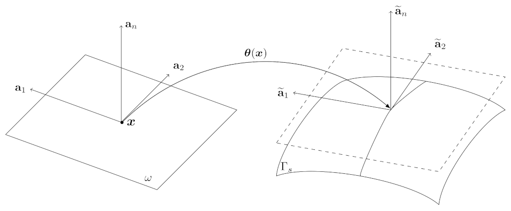
The Koiter shell approach relies on the assumption that the structure displacements are small and normal to the surface of the shell. Let
be a linear mapping between a reference fixed point and a generic point on the middle surface. We denote, with
, the points of the reference configuration and with
the deformed membrane configuration, as shown in
Figure 1.
We now consider the tangential base
, for
. Thus,
and
define the plane tangential to the shell, while
defines the unit vector normal. Now, we define the covariant metric tensor of the middle surface as
. Another fundamental tensor considered in this work is
The deformation can now be specified by the difference between
and
in the deformed and reference configuration. Subsequently, we introduce the strain measures
where
is the change of metric tensor, while
denote the covariant components of the linearized change of curvature tensor that is associated with a displacement
. In the rest of the paper, given a tensor
, we define
. The strain measures can be written in terms of the displacement components
, as
where the additional subscript preceded by a vertical stroke that is applied to the generic quantity
, e.g.,
, means the covariant surface differentiation with respect to the coordinate
.
In this work, we only consider normal displacements, thus there is not any change in length between the reference middle surface and the deformed one. Note that the normals are completely specified by arbitrary variations of
and
under the compatibility conditions (
1) and (
2). We can now introduce the linear Koiter shell equations. Let
be the considered shell domain, and let
be a measurable subset of
. In the following,
will denote the outer normal derivative operator along
. Because
, we can introduce the functional space
, such that
For more information regarding the introduced functional spaces and the derivation of the equations used in this section, see [
27]. We can define the energy functional of the Koiter shell equation as
where
and
is the thickness of the solid wall. The contravariant components of the shell elasticity tensor
are defined as
where
is the Poisson coefficient and
E the Young modulus of the solid material. The given functions
take the forces applied to the shell into account. We impose the boundary condition
on
, therefore the shell is clamped on the boundaries of its middle surface. For all of the admissible displacements
, we can derive the variational equation for the vector field
, as
In addition to the hypothesis of normal displacement, we also introduce the following assumptions: small deformations of the solid shell, negligible bending terms, and isotropic and homogeneous material. Therefore, we can neglect the term with
in Equation (
4). Moreover, we can assume
as a test function for the variational formulation, obtaining
If we restrict the membrane displacements to only normal direction, we can further simplify the variational formulation (
5), and reduce it to a simple scalar equation for
. In strong form, it reads
where
2.2. The Prestressed Term
The presented Koiter model does not account for prestressed loading, along with the shell structure. Let us consider the deformed non-shell configuration
. Note that
has thickness
, and the shell surface is defined as the middle surface of it. In a weak formulation, the prestress term is [
28]
where
is the Cauchy stress tensor in the deformed configuration for only tangential stresses in
. In the rest of this section, we will follow the procedure that is presented in [
18]. By taking the limit for
, we lead Equation (
8) back to the membrane case. Thus, we can write the deformation field as
Because the integration is performed on
, the terms where
appears are of higher order in
(in the order of
or more), so we can neglect them. The interested reader can see the full expansion in [
18]. Now, we introduce the surface covariant derivative of a vector field (see [
29]). The covariant derivative of
is defined as
With this notation, we can write the three-dimensional covariant derivatives of
as
Now by integrating (
8) and considering
, we have
Equation (
9) can be incorporated into the coefficient
in the Equation (
7). The Equation (10) gives a second derivative in space to be added inside the model (
6), obtaining
and
Model (
11) must be completed with the proper boundary conditions, i.e.,
. Note that the presented prestressed model can be used when the deformed configuration is close enough to the reference one, so we can consider an isotropic elastic tensor.
2.3. The Cylindrical Geometry
Let now consider a cylindrical geometry, in order to show how to explicitly calculate all of the introduced tensors in a simple three-dimensional geometry. If we consider a system of cylindrical coordinates and a cylinder of radius
R, we have
. The covariant basis is given by
this implies that
therefore
Subsequently, it is easy to show that
Moreover, because the prestress term acts only in the longitudinal dimension, in the cylindrical case we have
In this case, the system (
11) can be simplified as a one dimensional equation
where
. See [
30,
31] for more information on the applications of this model to hemodynamic.
2.4. The Coupled Fluid-Structure Model
The fluid is modeled as Newtonian, homogeneous, and incompressible. The fluid satisfies the following equations in ALE form [
2,
32]
where
and
are the density and the velocity vector of the fluid, respectively. The Cauchy stress tensor of the fluid is written as
, where
p and
are the pressure and dynamic viscosity of the fluid, respectively. The system of Equation (
14) is completed with appropriate boundary conditions. Moreover,
is the fluid domain and
is the ALE velocity that determines, step-by-step, the position of the nodes of the fluid domain as
.
In the following,
will denote the
inner product,
will denote the
inner product, and the bilinear form
is defined as
The optimal control that is introduced in this work is based on the stationary solution of the fluid–structure system. Therefore, in the following, we neglect all of the time derivatives. We can write the weak formulation for the fluid problem as
for all
and
and for all
.
With a similar approach, we can write the weak formulation for the prestressed shell Equation (
11), as
By using this shell model, the structure equations can be reduced to a boundary condition on
for the fluid problem. Therefore, the two sub-systems (
16) and (
17) are coupled by imposing
on
. Now, we define the functional space
, where
are the boundaries of
where Dirichlet conditions are imposed. In order to satisfy the continuity of the test functions
over the interface surface
in the coupled system, a new functional space is introduced as
Now, we can derive the weak form of the coupled final system by simplifying the two terms
and
. Note that
. Subsequently, the coupled system reads
for all
,
. A finite element technique is used to obtain the discrete weak formulation of (
19). With this approach, the structural equation can be incorporated in the fluid equations as Robin boundary conditions.
3. Optimality System
In this work, we are interested in solving a displacement matching optimal control problem. We aim to obtain a desired shell deformation profile by controlling the fluid pressure over a portion of its boundary. Therefore, the objective functional that we intend to minimize reads
The first term expresses the distance in norm between the actual displacement and its desired value over the controlled boundary , which can either be the whole moving wall or one sub-portion. The second term has been added to limit the -norm of the control, the fluid boundary pressure p. The regularization parameter weighs the importance of the two terms over the cost functional and the choice of its value can be challenging. As a general rule, too much regularization leads to smoother, but less effective, controls, while a lack of regularization may lead to numerical and convergence issues.
In this work, we use a standard Lagrange multiplier approach to derive the first-order necessary conditions. We first introduce the augmented functional
, which is obtained by adding to the objective functional
the FSI state Equation (
19) multiplied by the appropriate Lagrange multipliers, also known as adjoint variables.
Since our control variable is the fluid pressure on the boundary, we integrate by parts the contributions of the fluid stress tensor
. The surface integrals can be rewritten by substituting the definition of
. The stationary points of the Lagrangian functional can be found by setting to zero the Fréchet derivatives taken with respect to all the problem variables. When considering the variations of the adjoint variables, we recover the weak form of the state system (
19) and its boundary conditions. By taking the derivative in the direction
, we get
Because this derivative must vanish for every choice of
, then the volume term gives the following continuity equation for the adjoint velocity
while, by setting to zero the surface terms, we recover the following control equation over the controlled boundary
and the boundary conditions on
We remark that, where we impose Neumann boundary conditions with fixed pressure (i.e., ). we have .
Collecting the variations in the direction
, we have
We integrate by parts (
26), obtaining the equation for the boundary conditions of the adjoint velocity
We now collect
terms and integrate by parts, obtaining
which gives the equation for the adjoint velocity
with the boundary conditions
Moreover, we have to consider the change of
due to the motion of the boundary
along the direction
where
represents the shell curvature. Under the hypothesis of small deformations, we can safely neglect the terms where
appears. The term with
is defined on the surface
and a constant extension of this value towards the normal direction to the surface leads to a null normal gradient, so we have that the moving shape terms
vanish.
To summarize, the optimality system is composed by the state system (
19), by the control Equation (
24) and by the adjoint system (
23)–(
28) with boundary conditions (
25), (
27) and (
30). Since the optimality system doubles the number of the state variables, we use a segregated approach for the solution of the state, adjoint, and gradient equations. In this case, we can reuse the same solver for both the solution of the state (
19) and adjoint systems (
23)–(
28) with few modifications. In Algorithm 1, we describe the steepest descent method used.
| Algorithm 1 Description of the Steepest Descent algorithm. |
1. Set a state satisfying ( 19) ▹ Setup of the state - Reference case2. Compute the functional in ( 20) 3. Set fordo 4. Solve the system ( 23)–( 28) to obtain the adjoint state 5. Set the control update 6. Set while do ▹ Line search 7. Set 8. Solve ( 19) for the state with if then Line search not successful ▹ End of the algorithm end if end while end for
|
4. Numerical Results
In this section, we report some of the numerical results that were obtained by using the mathematical model shown in the previous sections. We implemented the presented Koiter FSI model in the multigrid finite element code FEMuS [
33], which relies on PETSc libraries for the solution of the multigrid discretized linear solver with MPI parallelization. We compare the results that were obtained with the presented Koiter FSI model with a simplified analytic problem. Subseequently, we further validate the implemented model through the comparison with a validated FSI model.
We also implemented the presented steepest descent algorithm in the code FEMuS, and we present different tests, showing the dependence of the optimal solution on the regularization parameter , the convergence with the grid refinement of the implemented algorithm, and the effectiveness of the used method when non-constant desired target fields are requested.
4.1. Validation of the Koiter FSI Model
Because the presented fluid–structure model based on Koiter shell equations is still not widespread, in the literature there are only a few works on a benchmarking of it. In this section, we will refer to the benchmarks that are present in [
34]. In particular, we first consider a simple numerical case, where an analytical solution is available. Another benchmark that is based on a comparison between the Koiter model and a fully validated monolithic fluid–structure model is then presented.
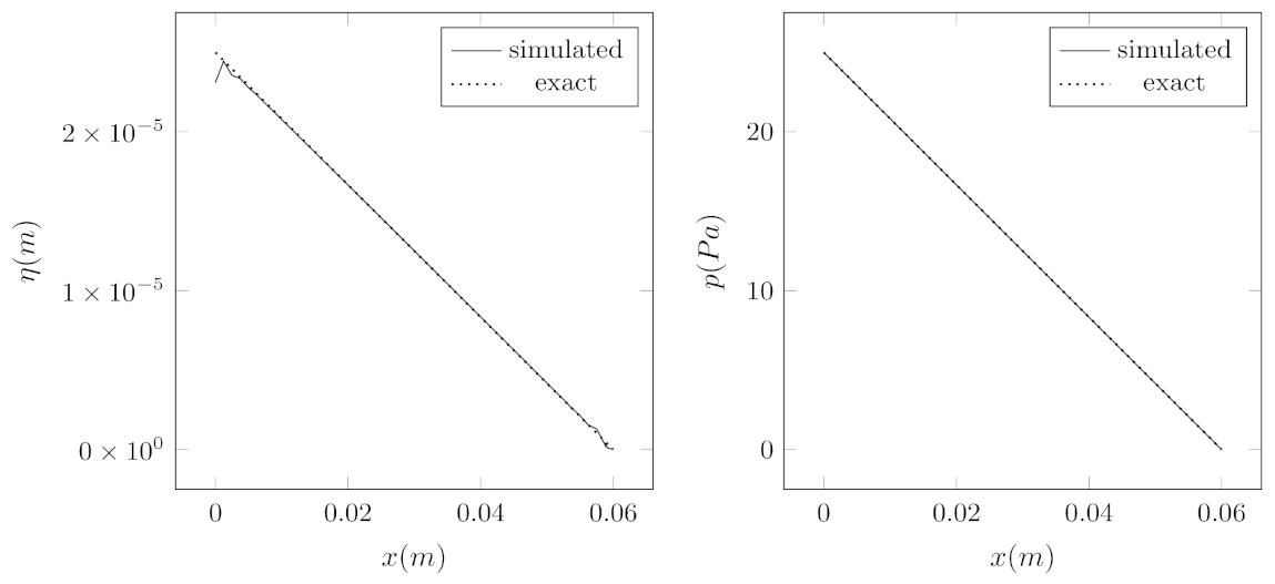
4.1.1. Exact Koiter Solution
We consider a fluid flowing through a cylindrical channel, obtained through the rotation of the rectangle around the z-axis, obtaining a cylinder of radius m and height m. We consider an inlet at the bottom and an outlet at the top. On the outer wall, the Robin boundary condition for Koiter shell is imposed. We consider a solid shell with density , a Poisson coefficient , an elastic modulus kPa, and a wall thickness m. Moreover, we consider a fluid with density and viscosity .
Since we are considering a cylindrical geometry, we consider the simplified model (
13). By neglecting the prestress term, the problem turns out to be linear, and can be exactly solved under certain conditions. By imposing a constant inlet pressure
, in fact, it is possible to obtain the analytical solution of the pressure and the displacement fields for stationary solutions.
Under the presented parameter setting we obtain kPa/m. Then, by setting a time step of s, an inlet pressure of Pa and an outlet pressure of Pa, after a time s the steady state is reached.
As mentioned in [
34], the fluid pressure is linear within the channel, as
Subsequently, the exact radial displacement of the structure is simply given by
The comparison between the displacement field that is simulated with the implemented algorithm and the exact displacement (
33) is reported in
Figure 2 on the left, showing good agreement between the expected and simulated values of the considered field. However, some discrepancies between the exact and the simulated solutions can be found at the extremes of the cylinders (at the inlet and outlet). This is due to boundary conditions on the displacement field that should be improved in future works. At the same time, in
Figure 2 on the right the comparison of the exact (
32) and the simulated pressure fields along the cylinder axis are reported. It can be seen that there is total agreement between the simulated pressure and the exact one.
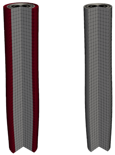
4.1.2. Comparison with a Validated FSI Model
The Koiter FSI model is now compared with the result of a monolithic fluid–structure model that is implemented in the FEMuS code and validated through the Turek FSI benchmarks [
1]. The validation and the introduction of the mathematical and numerical model can be found in [
35].
Differently from the benchmark that was proposed in [
34], we do not consider a multi-layer case, and the comparison is developed on a single solid layer. Because the monolithic model satisfies the Turek benchmark, we use it as a reference for the testing of the new algorithm. The test has been carried out using the same parameters of the previous test, with the only exception of the elastic modulus (
Pa) and the wall thickness (
m). From (
12), we obtain
kPa/m.
Because the benchmarks available in the literature usually involve transient problems, we consider the time-dependent Koiter model (see [
18] for more information) by reformulating (
13) as
Now, we consider a variable inlet pressure value as
where
kPa and
s. With all of the presented hypotheses, the two different tests have been carried out on the meshes that are presented in
Figure 3, with a time step
s. As boundary conditions, we impose an inlet of the fluid from the bottom and an outlet from the top. On the outer wall (external surface of the cylinders), structure conditions are imposed.
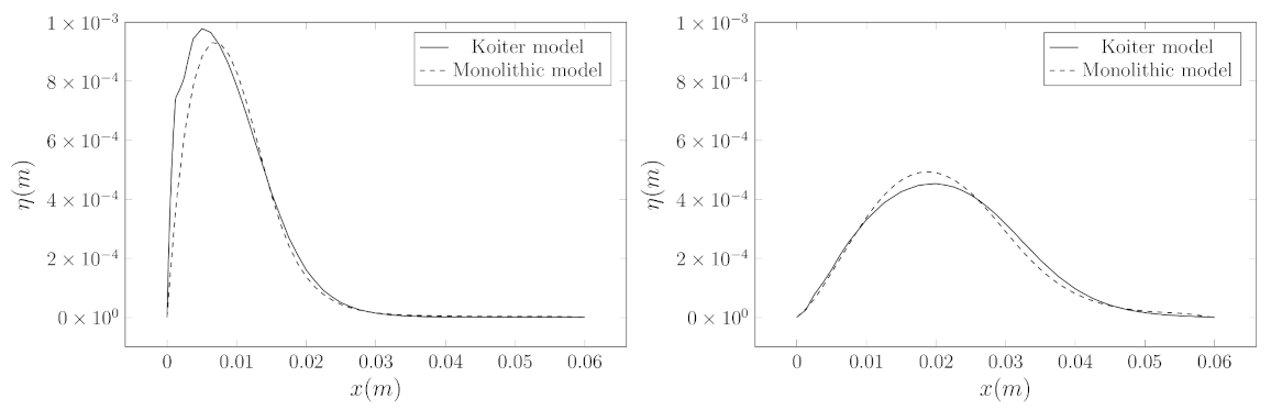
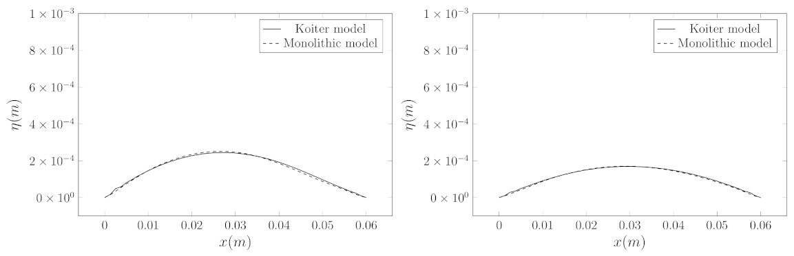
In
Figure 4 and
Figure 5, the comparison of the displacement field between the Koiter and monolithic model is reported. The displacement of the structure is calculated along the line between the two points
and
. It can be noted that the two models have similar behavior in time for all of the reported time steps. In particular, the two models differ from each other for
s and for
s. After the initial transition, the two solutions seem to converge to a similar solution, as can be seen for
s and
s.
Despite the slight differences between the Koiter and monolithic model noted above, from the presented preliminary results we can assert that the implement Koiter model is consistent with the solution that is obtained with the monolithic model, which has been fully tested in previous works.
Note that the reduction of the computational cost that i sobtained through the Koiter model depends on the solid mesh: the finer is the solid grid, the higher the reduction of the computational cost.
4.2. Regularization Term Tests
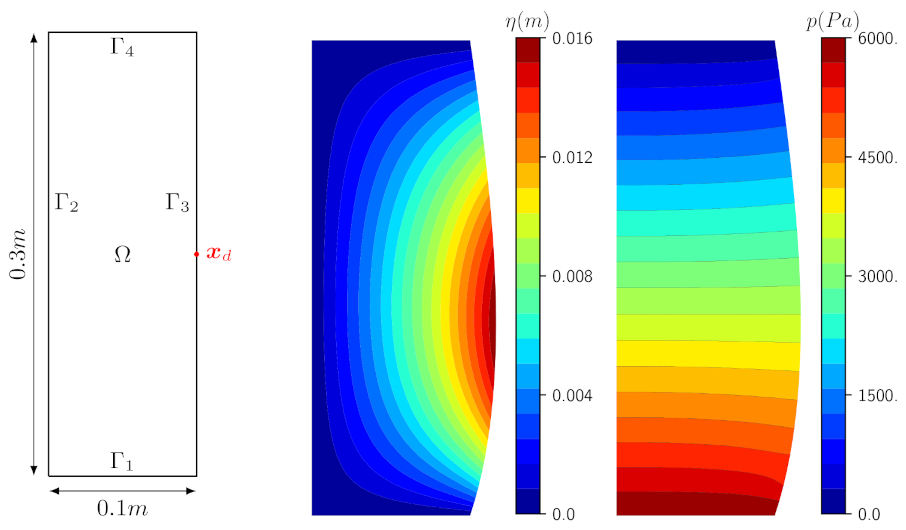
We now consider the numerical results of the implemented steepest descent algorithm. We show a simple numerical test to show the dependence of the implemented control algorithm for different values of the regularization term
. We consider the simplified case, where the domain
is reduced to a single point
. We consider a rectangular domain
, as shown in
Figure 6 on the left. The fluid has density
and dynamic viscosity
. For the solid, we consider
kPa/m and thickness
m. The domain is uniformly divided in a regular rectangular mesh.
We only present one simple case, where the fluid flows vertically from the bottom to the top. The region of the boundary
represents a solid wall with no-slip boundary condition (
) and
is the membrane where we impose the generalized Robin boundary condition (
6). As an initial condition, we impose a linear pressure field, decreasing from the bottom, where
Pa is imposed, to the top, where we fixed
Pa. In
Figure 6, we also report the steady solutions of the displacement field (center) and the pressure field (right) when the control algorithm is not considered.
The simulations aim to control the displacement of the point
of the membrane, in
direction, optimizing the pressure of the fluid on
. If we do not apply the control algorithm, the point
shows a displacement
m. The goal of this test is to reduce it to
m, thus changing the pressure of the fluid on
. Thus, the objective functional of the problem reads
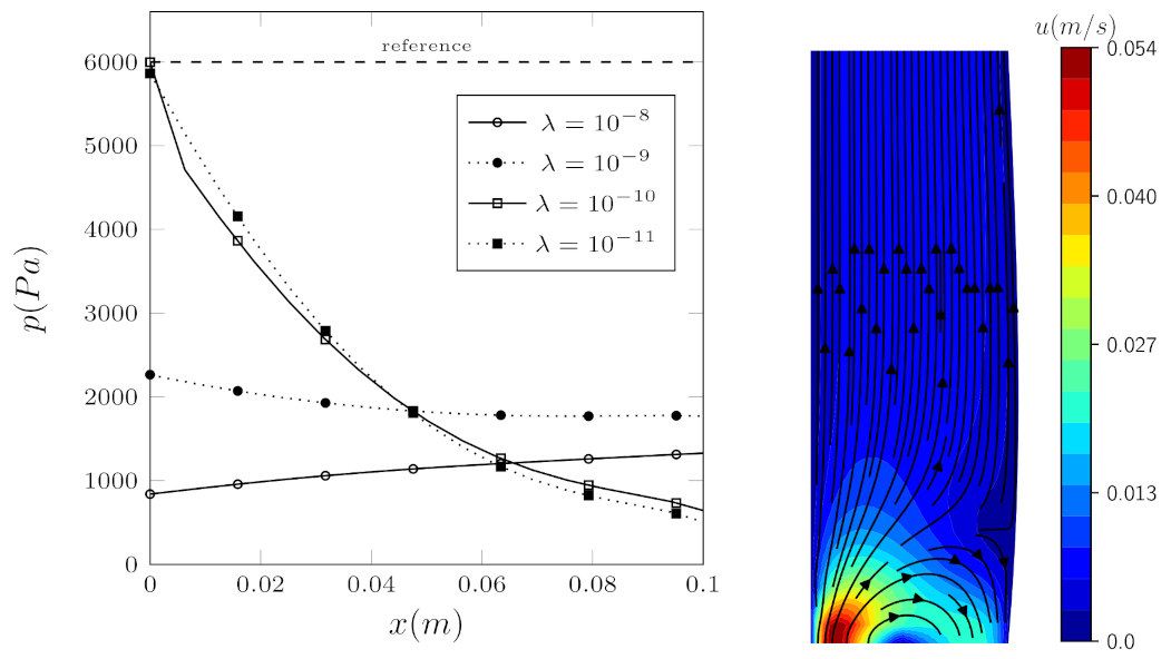
Table 1 presents the results of multiple simulations, with variations of the regularization parameter
, which has been introduced to regularize the control parameter
p and force it to the functional space
. Note that the solution is closer to the objective for small values of
. This result was expected, since, with larger
, the contribution of the regularization term in the minimization of the functional is more relevant. Thus, with larger
, we find smooth pressure profiles, but less precise displacement field
. In Table, we also report the number of iterations needed to the Algorithm 1 to find the optimal solution.
The controlled pressure
is updated via the formula
It clearly depends on the regularization parameter. In
Figure 7, the controlled pressure field along the boundary
is reported for various values of
. Note that the choice of the regularization parameter strongly affects the controlled pressure field, as expected. With less regularization, the objective term dominates in the functional and the pressure can have larger values, thus effectively controlling the membrane displacement. The comparison between the imposed reference initial condition and controlled pressure fields in all of the studied cases show that the control algorithm changes the solution on
in order to obtain the desired displacement
. Moreover, in
Figure 7 on the right, the velocity field for
is reported. Note that the pressure field that is imposed by the control algorithm forces an inverse flow at the inlet.
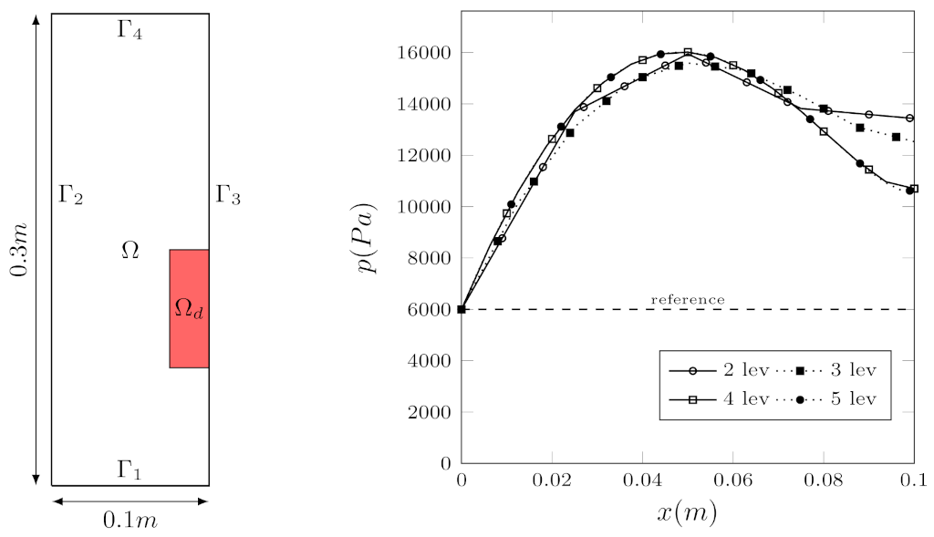
4.3. Grid Convergence Tests
Now, we show some results on the grid convergence of the proposed method. In particular, we require the reduction of the integral of the difference between and on when the grid is refined. Thus, we report different tests, depending on the requested displacement on .
In all of the considered cases, we consider the same physical values used in the last section. Moreover, we will consider
, unless stated otherwise. We consider a
mesh of the domain that is introduced in
Figure 8 on the left, and we refine it with a multi-grid approach. See [
36] and reference therein for more information regarding the multi-grid method.
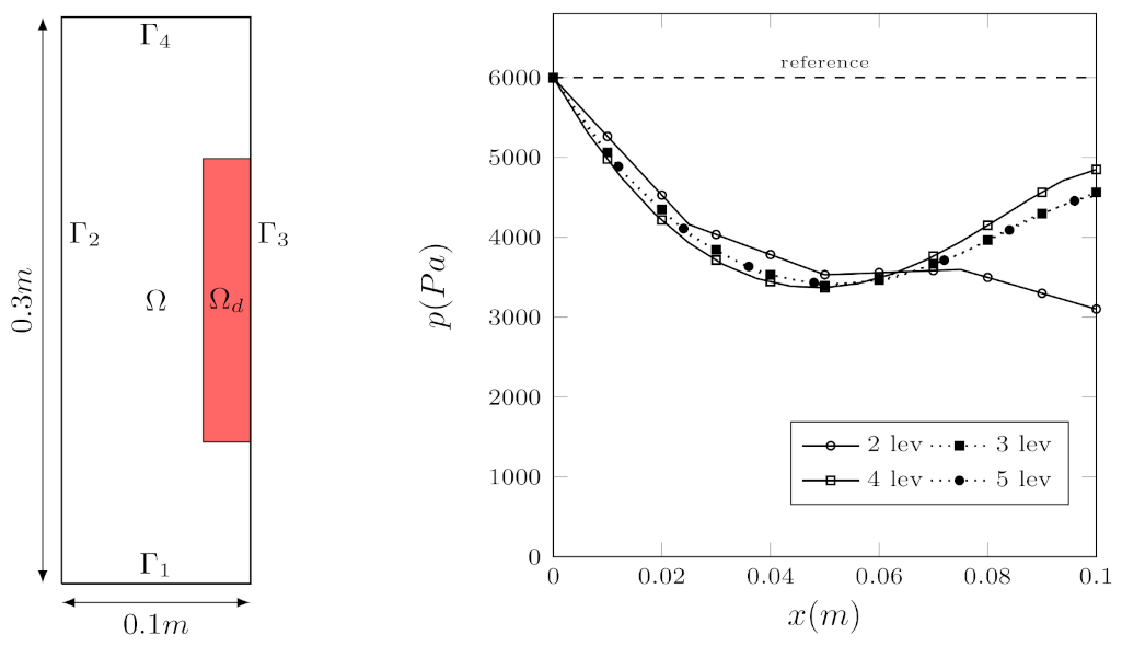
4.3.1. Displacement Reduction Test
We first compute a displacement reduction concerning the reference case, in which we request a desired displacement
m on
. We consider the geometry in
Figure 8 (left) with
. Moreover, we consider the same boundary conditions that were introduced in the last numerical test. We control the pressure
p field over
. The average displacement on
in the steady state without control case is
m. The functional that is associated with the presented control problem in all of the tests reported in the following reads
In
Figure 8 on the right, the comparison between the controlled pressure field for different grid refinements is reported along the controlled boundary
. In particular, all of the presented solutions seem to converge with the grid to a certain pressure field. All of the fields differ from the reference pressure field and, in particular, it can be noted that the pressure is reduced by the control algorithm at the inlet. This result is expected, since we are requesting a reduction of the displacement on
.
In
Table 2, the values of the distance between the desired solution and the solution found with the optimal control algorithm are reported. In particular, we compute the objective distance as
, where the integral over
is calculated on the same grid with the same quadrature rule for all of the considered grid refinements.
Note that the distance from the objective decreases when the refinement of the grid is increased. In
Table 2 , we also report the number of iterations of the algorithm to find the optimal solution. All of these values are compared with the reference simulation (no control,
). We also report the reduction rate, defined as
Note that all of the reported values of R are always . Therefore, the solution is always improved with respect to the reference one, which indicates that the control algorithm always finds a solution better than the reference solution.
4.3.2. Displacement Increase Test
Now, we consider a displacement increase with respect to the reference configuration. In particular, we request a desired displacement of
m on
, which is different when compared to the last considered case. We consider the domain that is reported in
Figure 9 on the left. All of the physical quantities are considered equal to the previous case. The average displacement field in
in the uncontrolled case is
m.
In
Figure 9, on the right, we report the comparison between the control pressure fields over
for different grid refinements. In particular, in contrast to the tests that were previously reported, a meaningful increase of the controlled pressure can be noted in this case. This is a direct consequence of the request for an increase of the desired displacement on
. Note that the pressure fields for 4 and 5 levels are coincident, as expected.
In
Table 3, the comparison between all of the tested cases is reported. In particular, all of the cases are compared with the reference one without control (i.e.,
). As in the previous case, we report the distance value from the objective calculated through the integral
. All of the controlled simulations show a minor distance from the objective when compared to the reference case. The reduction rate, as introduced in (
37), is
for all of the tested grids. This means that the solution always improves when compared to the reference one, and, for higher refinement levels, reduces the distance from the objective.
4.4. Non-Constant Desired Field Tests
We now consider a desired displacement field that depends on the position
. This test can be useful for practical applications where a non-constant objective is required. We present two different problems, with a sinusoidal and a step desired field. The geometry of the domain is reported in
Figure 8 (left), with
.
We consider a fluid density , fluid dynamic viscosity , and, for the approximation of the solid to mono-dimensional membrane, we consider kPa/m and thickness m. Moreover, we will consider , unless stated otherwise. We consider a mesh of the domain, refined 3 times with a multigrid technique. We consider an airbag-like case, therefore we impose a no-slip condition on , an inlet pressure on and the Koiter boundary condition on . We also have . We impose an inlet pressure of and consider .
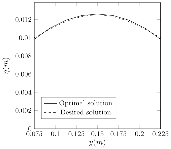
4.4.1. Sinusoidal Desired Displacement Test
We consider a simple sinusoidal case, where
is defined as
The shape of this function has been chosen to be easily reproduced while using the control strategy that is presented in this work.
In
Table 4, we report the distance from the objective, depending on the considered iteration of the implemented Steepest Descent algorithm. We also report the reduction rate, as defined in (
37). For simplicity, we only report the odd iterations. Note that the distance from the objective decreases in all the iteration of the optimization algorithm, and reach a final value of
. The final reduction rate of
suggests that the final solution is closer to the objective when compared to the initial solution.
In
Figure 10, the displacement field along the line
ℓ between the points
and
(such that
) is reported. Note that the optimal and reference solutions have a similar behavior; therefore, we can conclude that the optimization algorithm found a good solution, in agreement with the desired displacement.
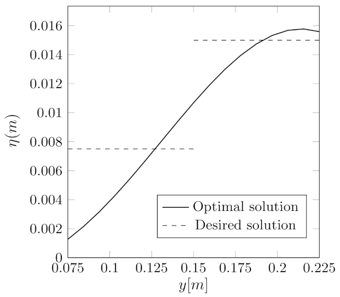
4.4.2. Step Function Desired Displacement Test
To test the presented algorithm on sharp desired functions, we now consider a step function
, defined as
All of the physical parameters are the same used in the last cases. Again, we consider an airbag case, where
. The presented case is not a straightforward control problem, since it is not easy to represent a step function displacement by controlling the pressure on
. We split the distance from the objective into two terms
and
, such that
where
and
with
.
In
Table 5, we report the values of
and
for various iterations of the algorithm. Note that the values of
and
are not uniformly decreasing with the algorithm iterations, but their sum does. In fact, the algorithm is designed to reduce the value of
: such value and, consequently, the reduction rate
R, decrease to the values
and
, respectively, after 9 iterations. The overall reduction rate indicates that the algorithm finds a solution that is consistently better than the initial one.
In
Figure 11, the displacement field along
ℓ is reported. It is very difficult to match perfectly the desired displacement
due to the nature of the desired function. The optimization algorithm works to minimize the distance between the optimal and desired solutions, and the solution that is found after 9 iterations of the optimization algorithm is reported in Figure. We remark that, even if the proposed optimal solution does not represent a perfect matching with the desired one, it is an upgrade of the initial solution by
times.
5. Conclusions
In this work, we have studied a fluid–structure interaction optimization problem based on a multi-scale model, where the thickness of the solid wall can be neglected and, therefore, greatly reduces rhe computational cost of the algorithm. We have stated the problem in monolithic form, where the membrane equation has been taken into account as a Robin boundary condition imposed on the moving boundary. We have obtained the optimality system of a pressure boundary control problem, to find a desired displacement of the membrane. The optimal control problem has been solved by using the Lagrange multiplier method and the gradient of functional has been determined by solving the adjoint problem.
The Koiter shell model has been validated through some numerical benchmarks, which involve the comparison with an analytical result on a simple case, and the comparison with a fully-validated monolithic FSI model.
Subsequently, a Steepest Descent algorithm has been introduced to solve the presented control problem, and it has been implemented in a finite element code. Some two-dimensional numerical tests have been introduced to validate the implemented algorithm. In particular, the dependence of the algorithm on the regularization parameter and its convergence with the grid refinement have been reported. The algorithm shows good convergence properties, and the dependence on the regularization term is consistent with the proposed mathematical model. Finally, the algorithm has been tested with non-constant objectives and, in particular, we considered a sinusoidal and a step-function desired displacement field. The algorithm found a sinusoidal solution in agreement with the desired one, and an improved, although not perfect, step-function solution.
The implemented algorithm has been proven to find a solution closer to the desired one in all of the tested cases in comparison to the uncontrolled solution. Moreover, better solutions are found as the regularization term tends to zero and the solutions converge with the grid refinement, as expected. Therefore, the presented algorithm aims to be an efficient tool for optimal boundary control problems that are applied to fluid–structure interaction simulations.
Author Contributions
Formal analysis, A.C., L.C. and S.M.; Investigation, A.C., L.C. and S.M.; Software, A.C., L.C. and S.M.; Validation, A.C., L.C. and S.M.; Writing—original draft, A.C., L.C. and S.M.; Writing—review & editing, A.C., L.C. and S.M. All authors have read and agreed to the published version of the manuscript.
Funding
This research received no external funding.
Conflicts of Interest
The authors declare no conflict of interest.
References
- Turek, S.; Hron, J. Proposal for numerical benchmarking of fluid-structure interaction between an elastic object and laminar incompressible flow. Lect. Notes Comput. Sci. Eng. 2006, 53, 371. [Google Scholar]
- Formaggia, L.; Quarteroni, A.; Veneziani, A. Cardiovascular Mathematics: Modeling and Simulation of the Circulatory System; Springer Science & Business Media: Milano, Italy, 2009; Volume 1. [Google Scholar]
- Bazilevs, Y.; Takizawa, K.; Tezduyar, T.E. Computational Fluid-Structure Interaction: Methods and Applications; John Wiley & Sons: Hoboken, NJ, USA, 2013. [Google Scholar]
- Le Tallec, P.; Mouro, J. Fluid structure interaction with large structural displacements. Comput. Methods Appl. Mech. Eng. 2001, 190, 3039–3067. [Google Scholar] [CrossRef]
- Sheldon, J.P.; Miller, S.T.; Pitt, J.S. Methodology for comparing coupling algorithms for fluid-structure interaction problems. World J. Mech. 2014, 4, 54. [Google Scholar] [CrossRef]
- ANSYS. Available online: https://www.ansys.com (accessed on 17 March 2021).
- Causin, P.; Gerbeau, J.F.; Nobile, F. Added-mass effect in the design of partitioned algorithms for fluid–structure problems. Comput. Methods Appl. Mech. Eng. 2005, 194, 4506–4527. [Google Scholar] [CrossRef]
- Nobile, F.; Vergara, C. Partitioned algorithms for fluid-structure interaction problems in haemodynamics. Milan J. Math. 2012, 80, 443–467. [Google Scholar] [CrossRef]
- Habchi, C.; Russeil, S.; Bougeard, D.; Harion, J.L.; Lemenand, T.; Ghanem, A.; Della Valle, D.; Peerhossaini, H. Partitioned solver for strongly coupled fluid–structure interaction. Comput. Fluids 2013, 71, 306–319. [Google Scholar] [CrossRef]
- Degroote, J.; Bathe, K.J.; Vierendeels, J. Performance of a new partitioned procedure versus a monolithic procedure in fluid–structure interaction. Comput. Struct. 2009, 87, 793–801. [Google Scholar] [CrossRef]
- Aulisa, E.; Bnà, S.; Bornia, G. A monolithic ALE Newton—Krylov solver with multigrid-Richardson—Schwarz preconditioning for incompressible fluid-structure interaction. Comput. Fluids 2018, 174, 213–228. [Google Scholar] [CrossRef]
- Failer, L.; Richter, T. A parallel Newton multigrid framework for monolithic fluid-structure interactions. J. Sci. Comput. 2020, 82, 28. [Google Scholar] [CrossRef]
- Cerroni, D.; Manservisi, S. A penalty-projection algorithm for a monolithic fluid-structure interaction solver. J. Comput. Phys. 2016, 313, 13–30. [Google Scholar] [CrossRef]
- Koiter, W. On the mathematical foundation of shell theory. In Proceedings of the International Congress of Mathematicians, Nice, France, 1 September 1970; Volume 3, pp. 123–130. [Google Scholar]
- Muha, B.; Canić, S. Existence of a weak solution to a nonlinear fluid–structure interaction problem modeling the flow of an incompressible, viscous fluid in a cylinder with deformable walls. Arch. Ration. Mech. Anal. 2013, 207, 919–968. [Google Scholar] [CrossRef]
- Maurits, N.; Loots, G.; Veldman, A. The influence of vessel wall elasticity and peripheral resistance on the carotid artery flow wave form: A CFD model compared to in vivo ultrasound measurements. J. Biomech. 2007, 40, 427–436. [Google Scholar] [CrossRef]
- Perktold, K. Mathematical modeling of local arterial flow. Comput. Methods Fluid-Struct. Interact. 1994, 306, 230. [Google Scholar]
- Nobile, F.; Vergara, C. An effective fluid-structure interaction formulation for vascular dynamics by generalized Robin conditions. SIAM J. Sci. Comput. 2008, 30, 731–763. [Google Scholar] [CrossRef]
- Chierici, A.; Chirco, L.; Giovacchini, V.; Manservisi, S.; Santesarti, G. A multiscale fluid structure interaction model derived from Koiter shell equations. J. Phys. Conf. Ser. 2020, 1599, 012040. [Google Scholar] [CrossRef]
- Gunzburger, M.D. Perspectives in Flow Control and Optimization; Siam: Philadelphia, PA, USA, 2003; Volume 5. [Google Scholar]
- Gunzburger, M.D.; Manservisi, S. Analysis and approximation of the velocity tracking problem for Navier–Stokes flows with distributed control. SIAM J. Numer. Anal. 2000, 37, 1481–1512. [Google Scholar] [CrossRef]
- Abergel, F.; Temam, R. On some control problems in fluid mechanics. Theor. Comput. Fluid Dyn. 1990, 1, 303–325. [Google Scholar] [CrossRef]
- Perego, M.; Veneziani, A.; Vergara, C. A Variational Approach for Estimating the Compliance of the Cardiovascular Tissue: An Inverse Fluid-Structure Interaction Problem. SIAM J. Sci. Comput. 2011, 33, 1181–1211. [Google Scholar] [CrossRef]
- Richter, T.; Wick, T. Optimal control and parameter estimation for stationary fluid-structure interaction problems. SIAM J. Sci. Comput. 2013, 35, B1085–B1104. [Google Scholar] [CrossRef]
- Chirco, L.; Manservisi, S. An adjoint based pressure boundary optimal control approach for fluid-structure interaction problems. Comput. Fluids 2019, 182, 118–127. [Google Scholar] [CrossRef]
- Chirco, L.; Manservisi, S. On the Optimal Control of Stationary Fluid–Structure Interaction Systems. Fluids 2020, 5, 144. [Google Scholar] [CrossRef]
- Ciarlet, P.G.; Mardare, C. An introduction to shell theory. Differ. Geom. Theory Appl. 2008, 9, 94–184. [Google Scholar]
- Bonet, J.; Wood, R.D. Nonlinear Continuum Mechanics for Finite Element Analysis; Cambridge University Press: Cambridge, UK, 1997. [Google Scholar]
- Lang, S. Introduction to Differentiable Manifolds; Springer Science & Business Media: Berlin/Heidelberg, Germany, 2002. [Google Scholar]
- Quarteroni, A.; Formaggia, L. Mathematical modelling and numerical simulation of the cardiovascular system. Handb. Numer. Anal. 2004, 12, 3–127. [Google Scholar]
- Quarteroni, A.; Tuveri, M.; Veneziani, A. Computational vascular fluid dynamics: Problems, models and methods. Comput. Vis. Sci. 2000, 2, 163–197. [Google Scholar] [CrossRef]
- Hughes, T.J.; Liu, W.K.; Zimmermann, T.K. Lagrangian-Eulerian finite element formulation for incompressible viscous flows. Comput. Methods Appl. Mech. Eng. 1981, 29, 329–349. [Google Scholar] [CrossRef]
- FEMuS Platform. Available online: https://github.com/FemusPlatform (accessed on 17 March 2021).
- Bukač, M.; Čanić, S.; Muha, B. A partitioned scheme for fluid–composite structure interaction problems. J. Comput. Phys. 2015, 281, 493–517. [Google Scholar]
- Chirco, L. On the Optimal Control of Steady Fluid Structure Interaction Systems. Ph.D. Thesis, Alma Mater Studiorum Università di Bologna, Bologna, Italy, 2020. [Google Scholar]
- Bramble, J.H. Multigrid Methods; Routledge: London, UK, 2018. [Google Scholar]
Figure 1.
Regular mapping between the reference shell surface and the deformed one .
Figure 1.
Regular mapping between the reference shell surface and the deformed one .
Figure 2.
Comparison of the displacement field (left) and the pressure p (right) between the simulated case and the reference one. The displacement field is reported along the line between the points and , and the pressure is reported along the cylinder axis.
Figure 2.
Comparison of the displacement field (left) and the pressure p (right) between the simulated case and the reference one. The displacement field is reported along the line between the points and , and the pressure is reported along the cylinder axis.
Figure 3.
The two meshes used for the numerical comparison between the monolithic (left, in red the solid domain) and the Koiter (right) FSI models. The two meshes have the same number of fluids elements.
Figure 3.
The two meshes used for the numerical comparison between the monolithic (left, in red the solid domain) and the Koiter (right) FSI models. The two meshes have the same number of fluids elements.
Figure 4.
Comparison between Koiter (continuous line) and the monolithic model (dashed line) displacement for s (left) and s (right).
Figure 4.
Comparison between Koiter (continuous line) and the monolithic model (dashed line) displacement for s (left) and s (right).
Figure 5.
Comparison between Koiter (continuous line) and the monolithic model (dashed line) displacement for s (left) and s (right).
Figure 5.
Comparison between Koiter (continuous line) and the monolithic model (dashed line) displacement for s (left) and s (right).
Figure 6.
Regularization term test. Geometry and controlled region (left), deformation (center) and pressure p (right) in in steady state without control.
Figure 6.
Regularization term test. Geometry and controlled region (left), deformation (center) and pressure p (right) in in steady state without control.
Figure 7.
Regularization term test. Control pressure p on with different regularization parameters (left). The dotted line represents the pressure in the reference case with no control (i.e., ). On the right: velocity in for .
Figure 7.
Regularization term test. Control pressure p on with different regularization parameters (left). The dotted line represents the pressure in the reference case with no control (i.e., ). On the right: velocity in for .
Figure 8.
Displacement reduction test. Comparison between the pressure field over for different mesh refinements (right). Controlled domain (left).
Figure 8.
Displacement reduction test. Comparison between the pressure field over for different mesh refinements (right). Controlled domain (left).
Figure 9.
Displacement increase test. Domain used for the grid convergence test with of dimension 0.025 m × 0.075 m (left). Comparison between the pressure field over for different mesh refinements (right).
Figure 9.
Displacement increase test. Domain used for the grid convergence test with of dimension 0.025 m × 0.075 m (left). Comparison between the pressure field over for different mesh refinements (right).
Figure 10.
Sinusoidal desired field test. Displacement field along the line between the points and .
Figure 10.
Sinusoidal desired field test. Displacement field along the line between the points and .
Figure 11.
Step function desired field test for Levels . Displacement field along the line between the points and .
Figure 11.
Step function desired field test for Levels . Displacement field along the line between the points and .
Table 1.
Regularization term test. Objective functional and displacement values obtained for different values. The total number of iteration of the algorithm is also reported.
Table 1.
Regularization term test. Objective functional and displacement values obtained for different values. The total number of iteration of the algorithm is also reported.
| () | (m) | Iterations |
|---|
| ∞ | | 0.015824 | - |
| | 0.002906 | 4 |
| | 0.004895 | 8 |
| | 0.004979 | 10 |
| | 0.004997 | 12 |
| | 0.005000 | 26 |
Table 2.
Displacement reduction test. Distance from the objective as a function of the number of refinement levels.
Table 2.
Displacement reduction test. Distance from the objective as a function of the number of refinement levels.
| Levels (ndof) | | ( | Iterations | R |
|---|
| ∞ | | - | - |
| | | 10 | |
| | | 10 | |
| | | 12 | |
| | | 10 | |
Table 3.
Displacement increase test. Distance from the objective as a function of the number of refinement levels.
Table 3.
Displacement increase test. Distance from the objective as a function of the number of refinement levels.
| Levels (ndof) | | ( | Iterations | R |
|---|
| ∞ | | - | - |
| | | 12 | |
| | | 7 | |
| | | 12 | |
| | | 11 | |
Table 4.
Sinusoidal desired displacement test. Distance from the objective and reduction rate R of the objective functional as a function of control algorithm iterations.
Table 4.
Sinusoidal desired displacement test. Distance from the objective and reduction rate R of the objective functional as a function of control algorithm iterations.
| It | | | R |
|---|
| - | ∞ | | - |
| 1 | | | |
| 3 | | | |
| 5 | | | |
| 7 | | | |
| 9 | | | |
Table 5.
Step function desired displacement test. Distance from the objective for both the domains and , and overall distance from the objective as a function of the algorithm iteration. The reduction rate R is also reported.
Table 5.
Step function desired displacement test. Distance from the objective for both the domains and , and overall distance from the objective as a function of the algorithm iteration. The reduction rate R is also reported.
| It | | | | | R |
|---|
| - | ∞ | | | | - |
| 1 | | | | | 5.43 |
| 3 | | | | | |
| 5 | | | | | |
| 7 | | | | | |
| 9 | | | | | |
| Publisher’s Note: MDPI stays neutral with regard to jurisdictional claims in published maps and institutional affiliations. |
© 2021 by the authors. Licensee MDPI, Basel, Switzerland. This article is an open access article distributed under the terms and conditions of the Creative Commons Attribution (CC BY) license (https://creativecommons.org/licenses/by/4.0/).


