Approximate Analytical Analysis of Unsteady MHD Mixed Flow of Non-Newtonian Hybrid Nanofluid over a Stretching Surface

Abstract

This paper analyses the two-dimensional unsteady and incompressible flow of a non-Newtonian hybrid nanofluid over a stretching surface. The nanofluid formulated in the present study is${\mathrm{TiO}}_2+\mathrm{Ag}+\mathrm{blood}$, and ${\mathrm{TiO}}_2+\mathrm{blood}$, where in this combination ${\mathrm{TiO}}_2+\mathrm{blood}$ is the base fluid and ${\mathrm{TiO}}_2+\mathrm{Ag}+\mathrm{blood}$ represents the hybrid nanofluid. The aim of the present research work is to improve the heat transfer ratio because the heat transfer ratio of the hybrid nanofluid is higher than that of the base fluid. The novelty of the recent work is the approximate analytical analysis of the magnetohydrodynamics mixed non-Newtonian hybrid nanofluid over a stretching surface. This type of combination, where ${\mathrm{TiO}}_2+\mathrm{blood}$ is the base fluid and ${\mathrm{TiO}}_2+\mathrm{Ag}+\mathrm{blood}$is the hybrid nanofluid, is studied for the first time in the literature. The fundamental partial differential equations are transformed to a set of nonlinear ordinary differential equations with the guide of some appropriate similarity transformations. The analytical approximate method, namely the optimal homotopy analysis method (OHAM), is used for the approximate analytical solution. The convergence of the OHAM for particular problems is also discussed. The impact of the magnetic parameter, dynamic viscosity parameter, stretching surface parameter and Prandtl number is interpreted through graphs. The skin friction coefficient and Nusselt number are explained in table form. The present work is found to be in very good agreement with those published earlier.

1. Introduction

In the history of fluid mechanics, the derivation of the boundary layer equation and the solution using similarity transformation is the most important area for the researcher. With the help of boundary layer theory, both Newtonian and non-Newtonian fluids can be modeled. The results obtained with the help of boundary layer theory have more similarity to the experimental work. The industrial application of non-Newtonian fluid is higher compared to Newtonian fluid because of the uses of non-Newtonian fluid in petroleum drilling polymer engineering, hot rolling wire and fiber coating, manufacturing of food, metal spinning glass fiber production and paper production, etc. Many nonlinear relations are observed for the stress and the rate of strain for non-Newtonian fluids; to express all those properties of non-Newtonian fluids in a single equation is difficult work. The flow due to the stretching sheet of the boundary layer of non-Newtonian fluid has some important application in several manufacturing fields. The non-Newtonian fluid model has a great deal of mechanical applications. The study of heat transfer in nanofluids is of great importance due to their many uses in various sectors.

In 1995, in the American Society of Mechanical Engineers winter annual conference, Choi [1] was the first scientist who introduced the term nanofluid. In the consideration of thermal assets, it is the core issue with traditional types of heat carrying fluids such as ethylene glycol, water, oil and lubricants, as they lack in the larger heat transport features. Nanofluid has invented a revolutionary modification in the field of fluid dynamics to enhance the thermal conductivity of conventional fluids. Several scientists have investigated the nanofluids, both experimentally and from a theoretical point of view. Accordingly, nanoparticles investigators yield various ingredients in order to make them useful in enhancing the thermal conductivity. Such nanoparticles contain ceramic (${\mathrm{Al}}_2{\mathrm{O}}_3,\mathrm{CuO}$), metals ($\mathrm{Ag},\mathrm{Cu},\mathrm{Au}$), ferro particles (${\mathrm{CoFe}}_2{\mathrm{O}}_4,{\mathrm{Fe}}_3{\mathrm{O}}_4,\mathrm{Mn}$-${\mathrm{ZnFe}}_2{\mathrm{O}}_4$), metal nitrides ($\mathrm{AlN},\mathrm{SiN}$) and carbon in various forms (diamonds, graphite and carbon nanotubes). Many studies have been conducted about nanofluids up to now, and hybrid nanofluid is one of the new types of nanofluid that has attracted the attention of researchers.

Hybrid nanofluids are produced in two forms. The first form is whereby two or more types of nanofluid are suspended in a base fluid, the second one is when nanoparticles are suspended in a base fluid like composite. In fact, the reason for researcher’s attention to this issue is that the heat transfer rate enhancement and production cost reduction can be achieved by application of these nanofluids. Hybrid nanofluids are presented to propose superior thermo-physical characteristics and excellent rheological behavior with enriched heat transport features. The hybrid nanofluids are the extension of nanoliquids containing two distinct nanoparticles scattered in a base fluid, a novel kind of heat transport fluid that attracts the consideration of many scientists. Hybrid nanofluids has been widely used in various sectors of heat transport, such as micro-electric, generator cooling, reduction of drugs, cooling of atomic system, refrigeration, cooling of transformers, etc. The concept of hybrid nanofluids has improved the progressive features of ordinary nanofluid that were discovered by Suresh et al. [2]. Recently, few numerical studies were examined on hybrid nanofluids as a new idea in the field of science and technology. Devi and Devi [3,4] examined the problems of the heat transfer and the flow of hydro-magnetic hybrid nanofluids ($\mathrm{Cu}$-${\mathrm{Al}}_2{\mathrm{O}}_3$-Water) over a stretching sheet. Tayebi and Chamkha [5] attended numerically the problem of heat transfer of $\mathrm{Cu}$-${\mathrm{Al}}_2{\mathrm{O}}_3$-Water hybrid nanofluids in an annulus. The characteristics of ${\mathrm{TiO}}_2$-$\mathrm{Cu}/{\mathrm{H}}_2\mathrm{O}$ hybrid nanofluid with Lorentz force was analyzed by Ghadikolaei et al. [6]. Hayat et al. [7] inspected the rotating flow problem of $\mathrm{Ag}$-$\mathrm{CuO}/\mathrm{Water}$ hybrid nanofluids. The aqueous titania–copper hybrid nanofluid stagnation point flow towards a stretching cylinder was investigated by Yousefi et al. [8]. Subhani and Nadeem [9] studied the behavior of $\mathrm{Cu}$-${\mathrm{TiO}}_2/{\mathrm{H}}_2\mathrm{O}$ hybrid nanofluid over a stretching surface. Coşkun [10] studied the analysis of convective straight and radial fins with temperature-dependent thermal conductivity using variational iteration method with comparison with respect to finite element analysis. The numbers of studies in the field of nanofluids has increased rapidly over the past decade. Despite some inconsistency in the reported result and insufficient understanding of the mechanism of heat transfer in nanofluids, it has emerged as a promising heat transfer fluid. In the continuation of nanofluids research, recently researchers have also tried to use hybrid nanofluids, which are engineered by suspending dissimilar nanoparticles either in a mixture or composite form. The idea of using hybrid nanofluids is to further improve the heat transfer and pressure drop characteristics by a trade-off between advantages and disadvantages of individual suspension attributed to good aspect ratios, better thermal networks and synergistic effects of the nanomaterial. There is a growth in the use of hybrid nanofluids in the biomedical industry for sensing and imaging purposes. This is directly related to the ability to design novel materials at the nanoscale level alongside recent innovations in analytical and imaging technologies for measuring and manipulating nanomaterials. This has led to the fast development of commercial applications, which use a wide variety of manufactured nanoparticles. The production, use and disposal of manufactured nanoparticles will lead to discharges into the air, soils and water systems. Negative effects are likely and the quantification and minimization of these effects on environmental health is necessary. True knowledge of the concentration and physicochemical properties of manufactured nanoparticles under realistic conditions is important to predicting their fate, behavior and toxicity in the natural aquatic environment. The aquatic colloid and atmospheric ultrafine particle literature both offer evidence as to the likely behavior and impacts of manufactured nanoparticles. The heat transfer application of hybrid nanofluids is used for industrial cooling that could result in great energy savings and resulting emissions reductions.

The phenomena of non-Newtonian liquid has a substantial impact on the innovation of renewable and sustainable energy processes for the development of contemporary trends. The Casson fluid model is an exceptional non-Newtonian liquid model that performs shearing thinning characteristics and stress. From such exclusive features, Casson fluid become an ideal rheological fluid model for human blood, as in the human body the red blood cells form rouleaux that create stress. Parmar et al. [11] examined the Casson model for blood flow with stenosed in blood vessel. Nadeem et al. [12] studied the effect of radiation and chemical reaction for Casson nanofluid. Ullah et al. [13] worked on non-Newtonian nanofluid flow through porous surface. The numerical results of Casson nanofluid flow in presence of joule heating and slip effect was investigated by Kamran et al. [14]. Additionally, the effect of radiation on energy expression over Casson nanofluid flow was examined by Archana et al. [15]. Gireesha et al. [16] investigated the Casson nanofluid flow and studied the impact of chemical reaction and radiation. Other than that study, the succeeding recent articles can be referred to the additional information associated to the Casson nanofluid flows, for example Souayeh et al. [17], Ullah et al. [18], Aziz and Afify [19]. Raza [20] discussed the thermal radiation and slip effects on magnetohydrodynamic (MHD) stagnation point flow of Casson fluid over a convective stretching sheet. Alkasassbeh et al. [21] discussed the effects of Stefan blowing and slip conditions on unsteady MHD Casson nanofluid flow over an unsteady shrinking sheet. Lund et al. [22] discussed the MHD flow of $\mathrm{Cu}$-${\mathrm{Fe}}_3{\mathrm{O}}_4/{\mathrm{H}}_2\mathrm{O}$ hybrid nanofluid with the effect of viscous dissipation according to the growing requirement of non-Newtonian hybrid nanofluid in engineering and industry areas. To overcome the issue of heat transfer rate enhancement and production cost reduction, the aim of the present work is the non-Newtonian hybrid nanofluid model that is an update on non-Newtonian hybrid nanofluid flow over a stretching surface. The analytical approximate method, the optimal homotopy analysis method (OHAM), is used for the model problem, as described by Liao et al. [23,24]. The impact of different parameters is interpreted through graphs. The skin friction coefficient and Nusselt number is explained in table form. The present work is found to be in very good agreement with those published earlier. The remaining paper is planned as follows: the literature review is presented in Section 1, the mathematical formulations of the important equation with the boundary conditions are derived in Section 2, the analysis of OHAM is presented in Section 3, the results and discussion are in Section 4, and the conclusion is presented in Section 5.

2. Mathematical Formulation

Consider the unsteady boundary layer stagnation point flow of non-Newtonian hybrid nanofluid ${\mathrm{TiO}}_2+\mathrm{blood}$ and ${\mathrm{TiO}}_2+\mathrm{Ag}+\mathrm{blood}$ over a stretching surface located at $y=0$ and the flow being confined in $y>0$, with stretching parameter $\lambda =\frac{b}{c}$ and magnetic field $M=\frac{\sigma B_0^2}{{\rho }_{nf}}$. The geometry of the flow problem is represented in Figure 1.

Under the above condition the boundary layer equation for the unsteady flow towards the stretching surface can be written as follows:

$$\frac{\partial u}{\partial x}+\frac{\partial v}{\partial y}=0$$

(1)

$$\frac{\partial u}{\partial t}+u\frac{\partial u}{\partial x}+v\frac{\partial u}{\partial y}=U_s\frac{d{U}_s}{dx}+k^{*}\frac{{\partial }^{2}u}{\partial y^2}-\frac{\sigma B_0^2}{{\rho }_{nf}}.$$

(2)

The temperature distribution in the flow field is as follows:

$$\frac{\partial T}{\partial t}+u\frac{\partial T}{\partial t}+v\frac{\partial T}{\partial t}=\frac{k}{\rho C_p}\frac{{\partial }^{2}T}{\partial y^2}.$$

(3)

The temperature is denoted by $T$, the thermal conductivity is denoted by $k$, the fluid density is denoted by $\rho$, and the specific heat is denoted by $C_p$. The velocity component along $x$ and $y$ is $u$ and $v$, respectively. The distance along the sheet is denoted by $x$ and the distance perpendicular to the sheet is denoted by $y$, the velocity of the stagnation point is denoted by $U_s=ax$ with $a>0$, the kinematic viscosity of the fluid is denoted by $k^{*}$, the magnetic field is denoted by $M$ and is defined as $M=\frac{\sigma B_0^2}{{\rho }_{nf}}$, the unsteady parameter is denoted by $\chi$ and is defined as $\chi =\frac{\gamma }{b}$, the Eckert number is defined as $Ec=\frac{U_{\varpi }^2}{C_p\left(T_{\varpi }-T_0\right)}$, $\lambda =\frac{b}{c}$ is the stretching parameter.

The boundary condition for velocity component is given as follows:

$$u=U_w,v=0\mathrm{at}y=0;u\to U_s\mathrm{as}y\to \infty .$$

(4)

The stretching velocity of the sheet is denoted by $U_w=cx$ where $c$ is the stretching constant. The boundary conditions for the temperature distribution were as follows:

$$T=T_w\mathrm{at}y=0;T\to T_{\infty }\mathrm{as}y\to \infty .$$

(5)

The temperature at the sheet is denoted by $T_w$ and the free stream temperature is denoted by $T_{\infty }$ which assume to be constant. The stream function is defined as follows:

$$u=\frac{\partial \psi }{\partial y}\mathrm{and}v=-\frac{\partial \psi }{\partial x}.$$

(6)

The similarity transformation is defined as follows:

$$\psi =\sqrt{\frac{a{\nu }_f}{1-\alpha t}}xf\left(\eta \right),\eta =y\sqrt{\frac{a}{{\nu }_f\left(1-\alpha y\right)}},\mathrm{and}\theta \left(\eta \right)=\frac{T-T_{\infty }}{T_w-T_{\infty }}.$$

(7)

The similarity transformation from Equation (7) is used in Equations (1)–(3). The similarity transformation satisfied Equation (1) identically and converts Equations (2) and (3) from nonlinear partial differential equations to nonlinear ordinary differential equations, as follows:

$$\begin{array}{c}\frac{1}{{\left(1-{\varphi }_1\right)}^{2.5}{\left(1-{\varphi }_2\right)}^{2.5}\left[\left(1-{\varphi }_2\right)\left(1-{\varphi }_1+{\varphi }_1\frac{{\rho }_{s_1}}{{\rho }_f}\right)+{\varphi }_2\frac{{\rho }_{s_2}}{{\rho }_f}\right]}{f}^{‴}-{\left(1-\varphi \right)}^{2.5}\left(\left(1-\varphi \right)+\varphi \frac{{\rho }_s}{{\rho }_{hnf}}\right)f^{″}f-f^{\prime 2}\\ -\chi {\left(1-\varphi \right)}^{2.5}M\left(\frac{\eta }{2}{f}^{″}+f^{\prime }\right)=0\end{array}$$

(8)

with boundary condition $f\left(\eta \right)=0,f^{\prime }\left(\eta \right)=\frac{c}{a}\mathrm{at}\eta =0$,

$$\frac{k_{nf}}{k_f}{\theta }^{″}-\left[\left(1-{\varphi }_2\right)\left(1-{\varphi }_1+{\varphi }_1\frac{{\left(\rho C_p\right)}_{s_1}}{{\left(\rho C_p\right)}_f}\right)+{\varphi }_2\frac{{\left(\rho C_p\right)}_{s_2}}{{\left(\rho C_p\right)}_f}\right]Pr\left({\theta }^{\prime }f\right)-\frac{\chi }{2}Ec\left(\eta {\theta }^{\prime }\right)=0$$

(9)

with boundary condition $\theta \left(\eta \right)=1\mathrm{at}\eta =0;\theta \left(\eta \right)\to 0\mathrm{as}\eta \to \infty$.

The skin friction coefficient $C_{nf}$ is defined as $C_{nf}=\frac{2{\tau }_{\varpi }}{\rho U_{\varpi }^2}$ and the local Nusselt number $N{u}_x=Nu=\frac{q_{\varpi }}{k\left(T_{\varpi }-T_0\right)}x$.

3. Analysis of OHAM

This approach is usually proposed by Liao [23,24] and applied to solve the boundary value functional equation. Consider the following boundary value functional equation:

$$\begin{array}{c}L\left(f\left(\eta \right)\right)+g\left(\eta \right)+N\left(f\left(\eta \right)\right)=0\\ B\left(f,\frac{df}{d\eta }\right)=0\end{array}$$

(10)

where $L$ and $N$ are linear and nonlinear operator, $g\left(\eta \right)$ is known function, $f\left(\eta \right)$ is unknown function and $B$ is the boundary operator. Consider the following deformation equations:

$$\begin{array}{c}\left(1-p\right)\left[L\left(f\left(\eta ,p\right)\right)+g\left(\eta \right)\right]=H\left(p\right)\left[L\left(f\left(\eta ,p\right)\right)+g\left(\eta \right)+N\left(f\left(\eta ,p\right)\right)\right]\\ B\left(f\left(\eta ,p\right),\frac{df\left(\eta ,p\right)}{d\eta }\right)\end{array}$$

(11)

where $p\in \left[0,1\right]$ is an embedding parameter, $H\left(p\right)$ for $p\ne 0$ is a nonzero auxiliary function such that $H\left(0\right)=0$ and $H\left(1\right)=1$. We have $f\left(\eta ,0\right)=f_0\left(\eta \right)$ and $f\left(\eta ,1\right)=f\left(\eta \right)$, respectively. Thus as $p$ increase from 0 to 1, the solution $f\left(\eta ,p\right)$ varies from $f_0\left(\eta \right)$ to $f\left(\eta \right)$, where $f_0\left(\eta \right)$ is an initial estimates that satisfies the linear operator which is obtained from Equation (11) for $p=0$:

$$\begin{array}{c}L\left(f_0\left(\eta \right)\right)+g\left(\eta \right)=0,\\ B\left(f_0,\frac{d{f}_0}{d\eta }\right).\end{array}$$

(12)

The auxiliary function $H\left(p\right)$ is consider as the following power series in $p$:

$$H\left(p\right)=C_{1}p+C_{2}p+\cdots$$

(13)

where $C_1$ and $C_2$ are constants that will be determined. The approximate analytical solution:

$$f\left(\eta ,p,C_1,\dots ,C_m\right)$$

(14)

is usually a power series about $p$ as follows:

$$f\left(\eta ,p,C_1,\dots ,C_m\right)=f_0\left(\eta \right)+{\displaystyle \sum }_{k\ge 1}{f}_k\left(\eta ,p,C_1,\dots ,C_m\right)p^k.$$

(15)

Substituting Equation (12) from Equation (15) and equating the coefficients of the terms with the identical power of $p$ leads to the governing equation $f_0\left(\eta \right),f_1\left(\eta \right)$ up to $f_k\left(\eta \right)$ which starts from Equation (12) that is:

$$\begin{array}{c}L\left(f_1\left(\eta \right)\right)=C_1{N}_0\left(f_0\left(\eta \right)\right),\\ B\left(f_1,\frac{d{f}_1}{d\eta }\right)=0.\end{array}$$

(16)

$$\begin{array}{c}L\left(f_k\left(\eta \right)-f_{k-1}\left(\eta \right)\right)=C_k{N}_0\left(f_0\left(\eta \right)\right)+{\displaystyle {\displaystyle \sum }_{i=1}^{k-1}}{C}_i\left[L\left(f_{k-1}\left(\eta \right)+N_{k-1}\left(f_0\left(\eta \right),f_1\left(\eta \right),\dots ,f_{k-1}\left(\eta \right)\right)\right)\right]\\ B\left(f_k,\frac{d{f}_k}{d\eta }\right)=0,k=2,3,\dots \end{array}$$

(17)

where $N_m\left(f_0\left(\eta \right),f_1\left(\eta \right),\dots ,f_m\left(\eta \right)\right)$ is the coefficients of $p^m$ obtained by expanding $N\left(f\left(\eta ,p,C_1,\dots ,C_m\right)\right)$ in a power series with respect to the embedding parameter $p$

$$N\left(f\left(\eta ,p,C_1,\dots ,C_m\right)\right)=N\left(f_0\left(\eta \right)+{\displaystyle \sum }_{k\ge 1}{N}_k\left(f_0\left(\eta \right),f_1\left(\eta \right),\dots ,f_k\left(\eta \right)\right)p^k\right)$$

(18)

where $N\left(f\left(\eta ,p,C_1,\dots ,C_m\right)\right)$ is given from Equation (15). The convergence of Equation (18) depends on the auxiliary constant $C_i,i=1,2,3,\dots$. If the Equation (18) converges when $=1$, one has:

$$f\left(\eta ,C_1,C_2,\dots ,C_m\right)=f_0\left(\eta \right)+{\displaystyle \sum }_{k\ge 1}{f}_k\left(\eta ,C_1,C_2,\dots \right).$$

(19)

The $m^{th}$ order approximation is given by:

$$f\left(\eta ,C_1,C_2,\dots ,C_m\right)=f_0\left(\eta \right)+{\displaystyle \sum }_{k\ge 1}^m{f}_k\left(\eta ,C_1,C_2,\dots ,C_m\right).$$

(20)

The result for the residual is defined as follows:

$$R\left(\eta ,C_1,C_2,\dots ,C_m\right)=L\left(f\left(\eta ,C_1,C_2,\dots ,C_m\right)+f\left(\eta \right)+N\left(f\left(\eta ,C_1,C_2,\dots ,C_m\right)\right)\right).$$

(21)

If $R\left(\eta ,C_1,C_2,\dots ,C_m\right)=0$ then $f\left(\eta ,C_1,C_2,\dots ,C_m\right)$ will be an exact solution and this is in general does not happened, especially in nonlinear problem. In order to find the optimal value of $C_i,i=1,2,\dots ,m$ we apply the method of least square.

$$\begin{array}{c}\frac{\partial J}{\partial C_1}=\frac{\partial J}{\partial C_2}=\dots =\frac{\partial J}{\partial C_m}=0\\ \mathrm{where}\end{array}$$

(22)

$$J\left(C_1,C_2,\dots ,C_m\right)={{\displaystyle \int }}_a^b{R}^2\left(\eta ,C_1,C_2,\dots ,C_m\right)d\eta ,$$

and the closed interval $\left[a,b\right]$ is the support of the given problem. Knowing these constants, the approximate solution of order $m$ will be determined easily.

4. Result and Discussion

The main objective of this section is to study the effect of the various model factors like $k^{*},M,\lambda ,Pr,Ec,\chi$ (kinematic viscosity, magnetic field, stretching parameter, Prandtl number, Eckert number, and unsteady parameter) on the velocity and temperature distribution. In

Table 1. Comparison of the skin friction for the two nanofluids when $Pr=15.6,k^{*}=0.9,A=0.1$

$\mathit{\chi }$	$\mathit{M}$	$\mathbf{Ti}{\mathbf{O}}_2+\mathbf{Blood}$	$\mathbf{Ti}{\mathbf{O}}_2+\mathbf{Ag}+\mathbf{Blood}$
0.7	1	0.929705	0.39471
0.8		0.92164	0.379547
0.9		0.91147	0.37264
	2	0.9100877	0.36994
	3	0.77608	0.33724
		0.768432	0.3246
		0.75818	0.31641

and

Table 2. Comparison of the Nusselt number ($R{e}_x^{-\frac{1}{2}}N{u}_x$) for the two nanofluids when $k^{*}=0.5,M=2,\lambda =0.7$.

$\mathit{P}\mathit{r}$	$\mathit{E}\mathit{c}$	$\mathbf{Ti}{\mathbf{O}}_2+\mathbf{Blood}$	$\mathbf{Ti}{\mathbf{O}}_2+\mathbf{Ag}+\mathbf{Blood}$
21	1.5	0.51231	0.49077
21.1	2.5	0.49341	0.48237
21.2	3.5	0.47451	0.47397
21.3	4.5	0.45614	0.45647
21.4	5.5	0.43776	0.44897
21.5	6.5	0.42795	0.43121
21.6	7.5	0.35021	0.41346

, the numeric results illustrate the impacts of different model factors on the skin friction coefficients and Nusselt number of both ${\mathrm{TiO}}_2+\mathrm{blood}$ and ${\mathrm{TiO}}_2+\mathrm{Ag}+\mathrm{blood}$. The skin friction coefficient decreases for the increasing value of the unsteady parameter and the magnetic field. The Nusselt number coefficient decreases for the increasing value of the Prandtl number and Eckert number.

The convergence for the approximate analytical solution has been obtained up to the 25th iteration in

Table 3. Convergence of the method for ${\mathrm{TiO}}_2+\mathrm{Ag}+\mathrm{Blood}$ when $Pr=6,M=10,Ec=1,k^{*}=1,\lambda =1$.

$\mathit{m}$	${\mathit{\epsilon }}_{\mathit{m}}^{\mathit{f}}\mathbf{Ti}{\mathbf{O}}_2+\mathbf{Ag}+\mathbf{Blood}$	${\mathit{\epsilon }}_{\mathit{m}}^{\mathit{\theta }}\mathbf{Ti}{\mathbf{O}}_2+\mathbf{Ag}+\mathbf{Blood}$
5	$1.36438\times {10}^{-1}$	$2.86775\times {10}^{-1}$
10	$7.14094\times {10}^{-3}$	$1.48738\times {10}^{-2}$
15	$5.209443\times {10}^{-7}$	$1.07298\times {10}^{-4}$
20	$4.37298\times {10}^{-9}$	$8.54131\times {10}^{-5}$
25	$3.95787\times {10}^{-11}$	$7.94423\times {10}^{-6}$

and

Table 4. Convergence of the method for ${\mathrm{TiO}}_2+\mathrm{Blood}$ when $Pr=6,M=10,Ec=1,k^{*}=1,\lambda =1$.

$\mathit{m}$	${\mathit{\epsilon }}_{\mathit{m}}^{\mathit{f}}\mathbf{Ti}{\mathbf{O}}_2+\mathbf{Blood}$	${\mathit{\epsilon }}_{\mathit{m}}^{\mathit{\theta }}\mathbf{Ti}{\mathbf{O}}_2+\mathbf{Blood}$
5	$1.07991\times {10}^{-1}$	$2.88574\times {10}^{-1}$
10	$5.65266\times {10}^{-2}$	$1.0759\times {10}^{-3}$
15	$4.12383\times {10}^{-3}$	$1.0759\times {10}^{-5}$
20	$3.4616\times {10}^{-4}$	$8.55721\times {10}^{-7}$
25	$3.133\times {10}^{-5}$	$8.006632\times {10}^{-9}$

, one by one. The increasing the number of iterations reduces the order of residual error and a strong convergence attained.

Table 5. Exhibits the thermo-physical properties.

Properties	Nanofluid	Hybrid Nanofluid
Density	${\rho }_{nf}=\left(1-\varphi \right){\rho }_f+\varphi {\rho }_s$	${\rho }_{hnf}=\left(1-{\varphi }_2\right)\left(1-{\varphi }_1\right)+{\varphi }_1{s}_1+{\varphi }_2{\rho }_2$
Heat capacity	${\left(\rho C_p\right)}_{nf}=\left(1-\varphi \right){\left(\rho C_p\right)}_f+\varphi {\left(\rho C_p\right)}_s$	$\begin{array}{c}{\left(\rho C_p\right)}_{hnf}=\left(1-{\varphi }_2\right)\left(1-{\varphi }_1\right){\left(\rho C_p\right)}_f+{\varphi }_1{\left(\rho C_p\right)}_{s_1}\\ +{\varphi }_2\rho {\left(\rho C_p\right)}_{s_2}\end{array}$
Viscosity	${\mu }_{nf}=\frac{{\mu }_f}{{\left(1-\varphi \right)}^{2.5}}$	${\mu }_{hnf}=\frac{{\mu }_f}{{\left(1-{\varphi }_1\right)}^{2.5}{\left(1-{\varphi }_2\right)}^{2.5}}$
Thermal conductivity	$\frac{k_{nf}}{k_f}=\frac{k_s+\left(n-1\right)k_f-\left(n-1\right)\varphi \left(k_f-k_s\right)}{k_s+\left(n-1\right)k_f+\varphi \left(k_f-k_s\right)}$	$\frac{k_{hnf}}{k_{bf}}=\frac{k_{s_2}+\left(n-1\right)k_{bf}-\left(n-1\right){\varphi }_2\left(k_{bf}-k_{s_2}\right)}{k_{s_2}+\left(n-1\right)k_{bf}+{\varphi }_2\left(k_{bf}-k_{s_2}\right)}$

exhibits the thermo-physical properties.

Figure 2 shows the influence of the magnetic field against the velocity field. The relation between $f^{\prime }\left(\eta \right)$ and $M$ is inversely related. For the growing magnitude of $M$ decreases the $f^{\prime }\left(\eta \right)$.

Physically, by increasing the magnetic field $M$, resistance forces are produced so that it decreases the velocity profile. Figure 3 shows the effect of the unsteady parameter $\chi$ on the velocity profile. For increasing the value of the unsteady parameter $\chi$ the velocity field $f^{\prime }\left(\eta \right)$ is decreasing in both the base nanofluid and hybrid nanofluid.

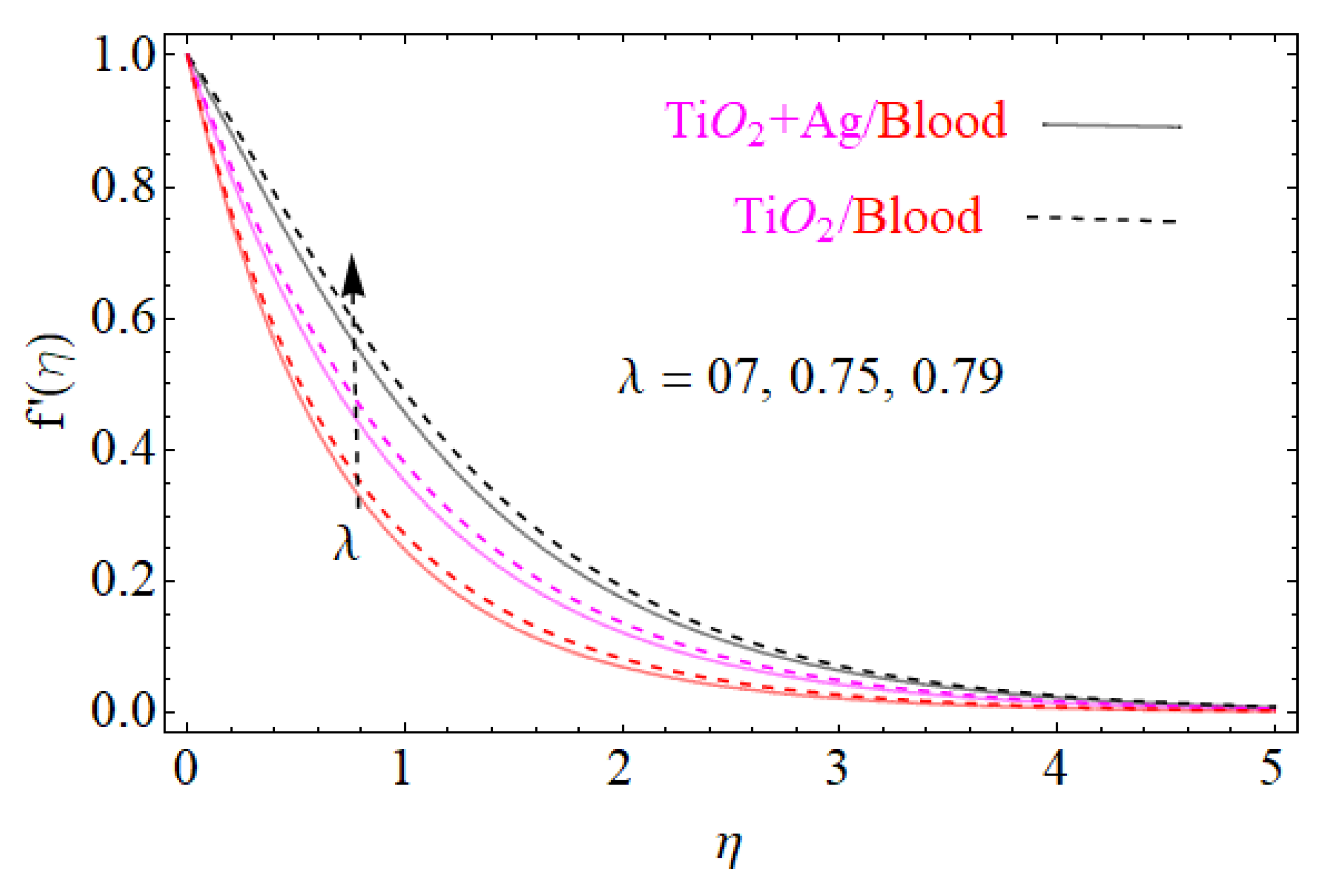
Figure 4 shows the effect of the stretching parameter $\lambda$ against the velocity equation. The velocity profile is the increasing function of the stretching surface. The increasing values of the stretching parameter $\lambda$ increase the $f^{\prime }\left(\eta \right)$ velocity field. Physically, by increasing the stretching parameter $\lambda$, the position of the fluid particle changes, so as a result the movement of the particle increases, so the velocity field is increasing by increasing of the stretching parameter $\lambda$.

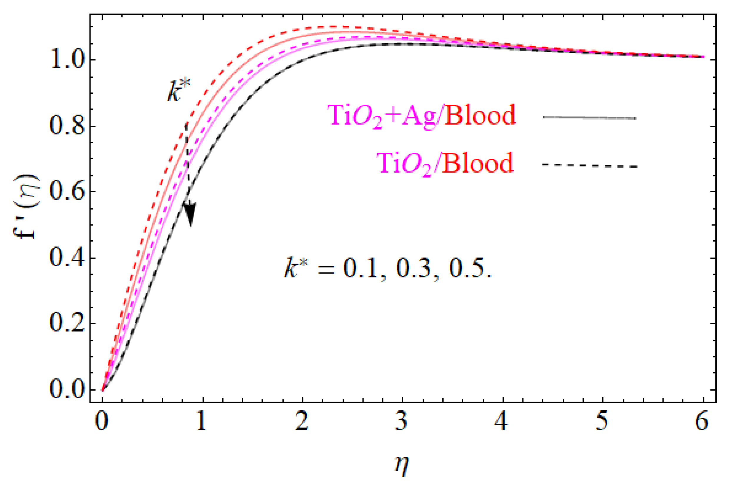
Figure 5 presents the effect of the kinematic viscosity on the velocity field. The increasing values of the kinematic viscosity $k^{*}$ decrease the $f^{\prime }\left(\eta \right)$ velocity field.

Physically, by increasing the kinematic viscosity, it produces resistant forces due to which fluid particles do not move easily, so as a result the velocity field is decreasing with the increasing of the kinematic viscosity.

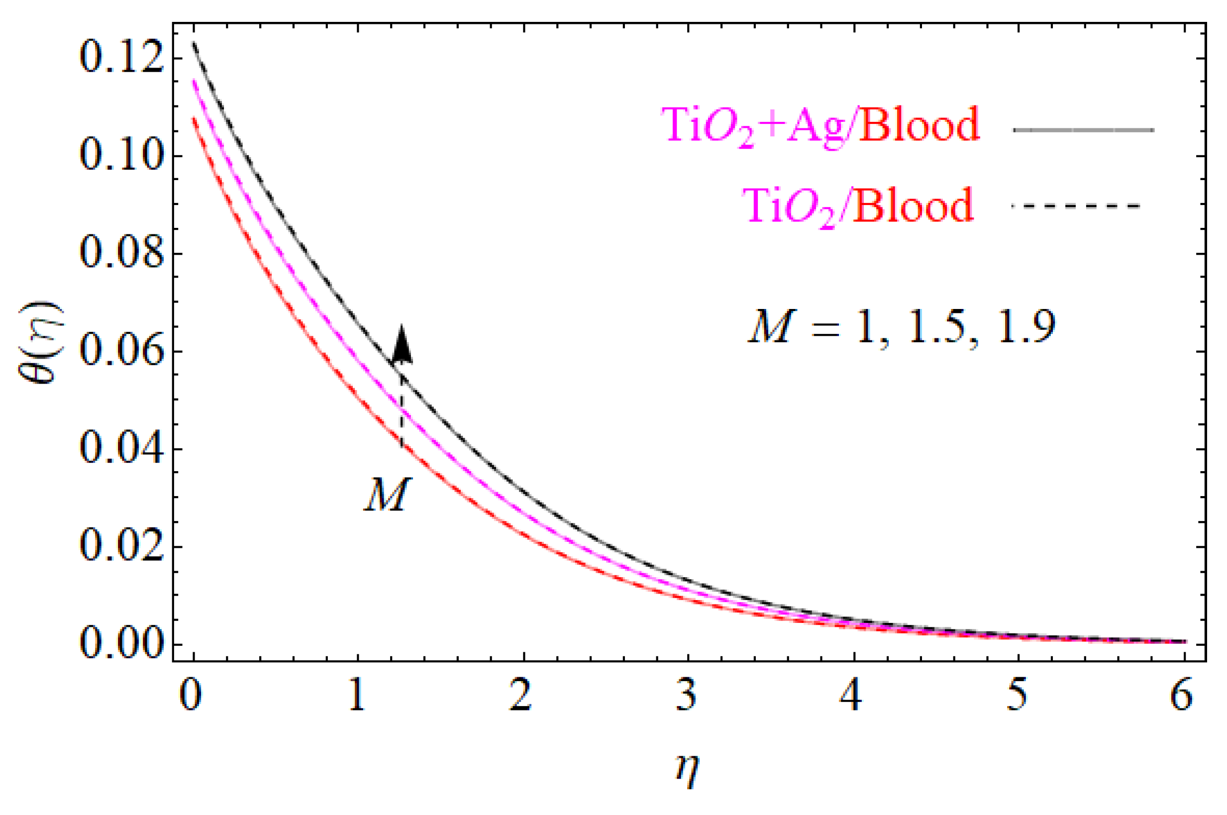
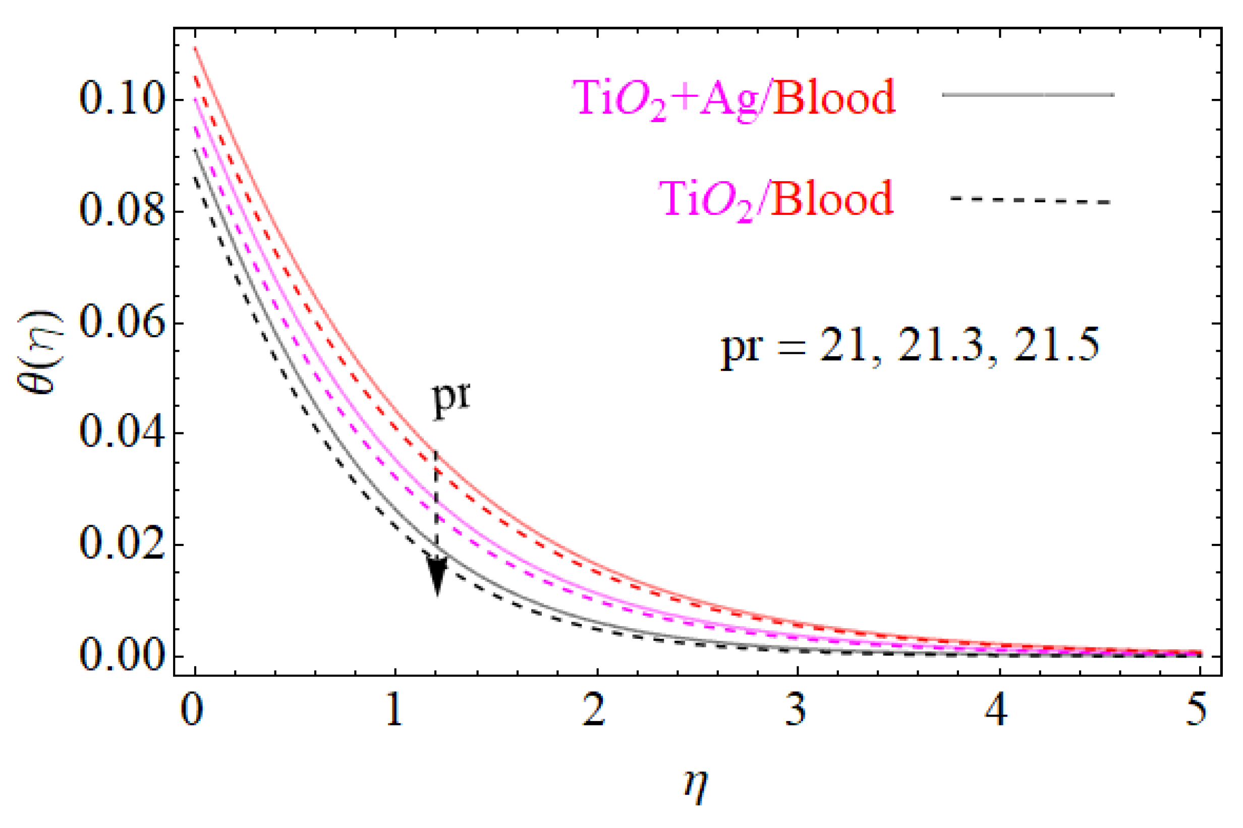
Figure 6 shows the effect of the magnetic field against the temperature profile. We see that by increasing the value of the magnetic field, the temperature profile decreases. Figure 7 shows the effect of the $Pr$ against the $\theta \left(\eta \right)$ temperature field:

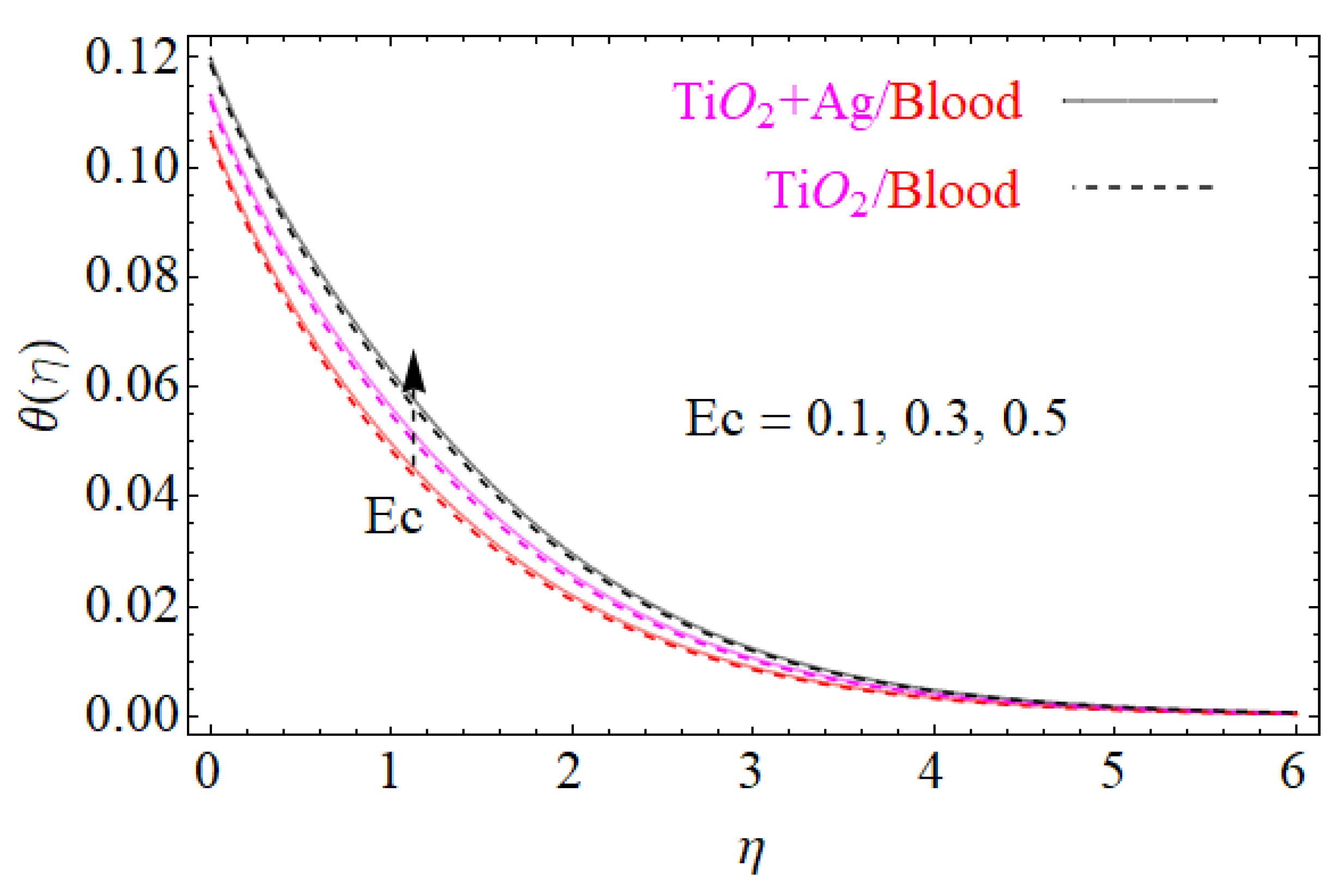
By enhancing the $Pr$, it decreases the temperature profile. In fact, the thickness of the momentum boundary layer is bound to be larger than that of the thermal boundary layer, or the viscous diffusion is larger than the thermal diffusion and therefore, the larger amount of the $Pr$ reduces the thermal boundary layer. Figure 8 shows the impact of the Eckert number versus the temperature field.

We notice that the relation between the temperature field and $Ec$ is directly related, that is, the increasing of $Ec$ increases the temperature profile as displayed in Figure 8. In fact, the thickness of the momentum boundary layer is smaller than that of the thermal boundary layer, or the viscous diffusion is less than the thermal diffusion and therefore, the larger value of the $Ec$ increases the thermal boundary layer.

5. Conclusions

This paper reports on the approximate analytical solution of the nonlinear differential equation. The fundamental partial differential equations are transformed to a set of nonlinear ordinary differential equations with a guide of some appropriate similarity transformation. The approximate analytical method, namely the OHAM is used for the model problem. The impact of the different parameters are interpreted through graphs. The skin friction coefficient and Nusselt number are explained in table form. The present work is found to be in very good agreement with those published earlier. The main outcomes of the present analysis were as follows:

• By increasing the unsteady parameter $S$, it decreases the velocity field.
• By increasing the stretching parameter $\lambda$, it increases the velocity profile.
• By increasing the Prandtl number $Pr$, it decreases the temperature profile.
• By increasing the Eckert number, it increases the temperature field.
• By increasing the magnetic field $M$, it decreases the velocity field.