100 m Resolution Age-Stratified Population Grid Data for China Based on Township-Level in 2020

Abstract

China’s age structure is undergoing profound demographic shifts, making accurate spatial information on age-stratified populations essential for policy-making, resource allocation, and risk assessment. However, census data are primarily aggregated by administrative units, offering coarse spatial resolution that constrains their integration and application with other gridded datasets. Using township-level population counts for four age groups (0–14, 15–59, 60–64, and ≥65 years) from the 2020 Seventh National Population Census across 38,572 townships, we developed an age-stratified downscaling framework. This framework integrates a random forest model with age-filtered Points of Interest (POI) data and other multi-source geospatial covariates to generate a 100 m resolution age-stratified population density weighting layer. Through township-level data dasymetric mapping, we produced the township-based 100 m Age-Stratified Population Grid Data (Township-ASPOP). Since township-level data represent the finest publicly available spatial unit of demographic statistics in China, we further validated the accuracy of Township-ASPOP by generating County-based 100 m Age-Stratified Population Grid Data (County-ASPOP) through dasymetric mapping using county-level age-stratified population data. The results demonstrate that County-ASPOP achieves superior predictive accuracy, with R² values of 0.95, 0.95, 0.85, and 0.86, and Root Mean Square Error (RMSE) values of 1743, 6829, 900, and 2033 persons per township for the four age groups, respectively—significantly outperforming the contemporaneous WorldPop dataset (R² = 0.69, 0.72, 0.64, and 0.60). The accuracy of Township-ASPOP is no less than that of County-ASPOP and effectively captures realistic spatial settlement patterns. This study establishes a reproducible framework for generating age-stratified population grid data and provides critical data support for policy formulation and resource allocation.

1. Introduction

Population structure is central to national development planning and the sustainable development agenda. Over the past fifty years, China has undergone significant demographic transitions, characterized by accelerated population aging and declining fertility rates [1,2]. Against this background, accurate, high-resolution, age-stratified population data are indispensable for informed policy formulation, precise resource allocation, and effective risk assessment [3,4,5]. However, a primary challenge persists: census data in China are predominantly aggregated by administrative units (e.g., counties). This aggregation not only restricts their seamless integration with other gridded geospatial datasets but also obscures the substantial population heterogeneity within these large units, thereby complicating accurate estimation [6,7,8,9]. Gridded population mapping has emerged as a powerful solution to this modifiable areal unit problem (MAUP), enabling the conversion of aggregated statistics into continuous surfaces [10,11].

Over the past three decades, methodologies for population downscaling have evolved significantly, primarily falling into two categories: areal interpolation and statistical modeling. Simple areal interpolation techniques, such as areal weighting [12], inverse distance weighting (IDW) [13], and kriging [14], redistribute population counts based solely on geometric properties, often failing to capture intra-zonal heterogeneity [15], as seen in GPWv4. To address this, dasymetric mapping incorporates auxiliary data, typically land use/cover, to assign weights non-uniformly [16,17]. Recent advancements have seen the rise of hybrid frameworks that integrate the strengths of both. A prominent example is the “intelligent” dasymetric mapping employed by WorldPop Global 2015–2030 Gridded Population Dataset (R2025A version v1, hereafter “WorldPop”), which combines statistical models (e.g., Random Forest) with remote sensing data to produce high-resolution global population estimates [18].

Recent studies have leveraged these advanced techniques and the increasing availability of geospatial big data. For instance, some studies have integrated multisource remote sensing imagery and Points of Interest (POI) within Random Forest models to generate national-scale 100 m population maps in China, demonstrating superior accuracy over existing products like WorldPop [19,20,21,22]. Other efforts have utilized ensemble learning [20] and novel approaches considering facility-based service capacity [8,23] to further refine population estimates. However, despite these progresses, three critical gaps remain in China. First, many studies still rely on county-level census data as the source, which is coarser than the publicly available township-level data from the latest 2020 Chinese census. In fact, some counties in western China are even larger than certain cities in the eastern regions, further exacerbating the mismatch between administrative boundaries and population distribution. Utilizing township-level data significantly minimizes the scale mismatch with target grid cells, a key factor known to enhance downscaling accuracy [22,24,25]. Second, most existing studies in China have focused on national-level downscaling of total population data [26,27,28,29], lacking comprehensive national-scale age-stratified population downscaling. Finally, although the value of POI data is widely acknowledged, studies that differentiate POI categories for different age groups remain relatively scarce. POI categories exhibit varying explanatory power for different demographic groups [8,23]; for example, educational POIs are more relevant to children, while medical facilities are more closely associated with the elderly. Most existing gridded population datasets for China, including the WorldPop [30], may lack this age-stratified refinement of variables, limiting their ability to accurately depict the spatial patterns of specific age groups.

To address these gaps, this study introduces a novel age-stratified downscaling framework for China with several key methodological advancements. (1) We utilize the most detailed township-level population counts from the 2020 Seventh National Population Census, minimizing source zone scale error. (2) We develop and incorporate age-stratified POI variables, identifying and weighting POI categories most relevant to each of the four age groups (0–14, 15–59, ≥60, and ≥65 years) to better capture the activity spaces of different demographics. (3) We apply a national settlement mask to constrain population allocation to inhabited areas, eliminating unrealistic predictions in uninhabitable zones. By integrating these elements within a robust Random Forest model, we generate a set of 100 m resolution age-stratified (age 0–14; age 15–59; age 60–64; age ≥ 65) gridded population datasets for China in 2020 (ASPOP). We rigorously evaluate our results against the contemporary WorldPop to quantitatively demonstrate the improvements in accuracy and spatial realism achieved by our approach.

2. Data Sources

Table 1 outlines the 2020 data used for fitting the Random Forest (RF) model and evaluating the accuracy of age-stratified population estimates corrected with county-level census data. Specifically, the 2020 township-level population data for China were initially used to calculate population density, which was then transformed using the natural logarithm to serve as the dependent variable in the model. Processed data on Points of Interest (POI), Nighttime Light (NTL), Slope, Elevation, the National Road Network, and a 100 m gridded population dataset of China’s 7th National Population Census (PopSE) [31] were aggregated to the township level and used as the independent variable for model training. Additionally, county-level population data were used as population control data in the subsequent dasymetric mapping procedure. County-based 100 m Age-Stratified Population Grid Data (County-ASPOP), which was corrected using county-level census data, were validated and compared for accuracy with the same-year WorldPop Global 2015–2030 Gridded Population Dataset (R2025A version v1). All datasets were initially reprojected to the Krasovsky_1940_Albers projection and then resampled to a 100 m resolution using bilinear interpolation for further analysis. The specific processing steps for each dataset are described below.

Table 1. Datasets used in this study.

Dataset	Format	Year	Scale	Source
Census population data	Table	2020	-	National Bureau of Statistics of China; Seventh National Population Census totals (county and township)
Boundary maps	Polygon	2020	-	National Geomatics Center of China (NGCC); Administrative divisions
POIs	Point feature	2020	-	Amap services, China
Nighttime lights	Grid	2020	1 km	National Earth System Science Data Center, National Science & Technology Infrastructure of China [32]
Elevation	Grid	-	30 m	NASA Earthdata [33]
Slope	Grid	-	30 m	NASA Earthdata [33]
Road network	Line feature	2020	-	Open Street Map (OSM)
PopSE	Grid	2020	100 m	figshare [31]
WorldPop (R2025A version v1)	Grid	2020	100 m	WorldPop Hub [30]

2.1. National Population Census of China

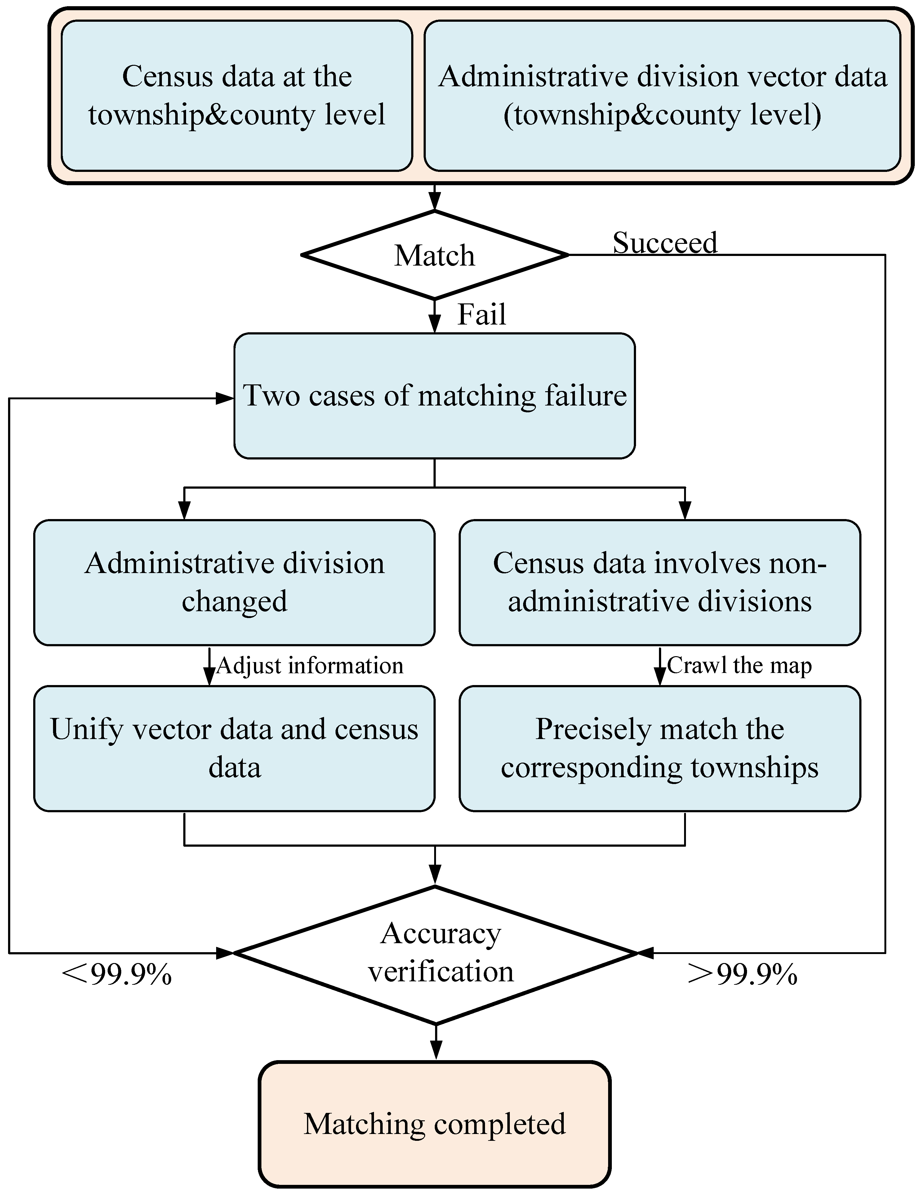
This study uses the 2020 Seventh National Population Census of China at the county and township levels (excluding Hong Kong, Macao, and Taiwan). Township-level counts were converted to population density and used as the dependent variable to maximize the accuracy of population estimates [12,34]. Before modeling, the township-level census data were matched with the township-level administrative boundary vector data (Figure 1). We first established a unique identifier by constructing a “Province–County–Township” system to automate the matching process. Records that were successfully matched proceeded to the next step. If matching failed, there were primarily two causes: (1) boundary or code changes due to administrative adjustments, and (2) the inclusion of non-standard administrative units, such as industrial parks or farms, in the census data. For the first case, we referred to the China Administrative Division website (http://www.xzqh.org (accessed on 24 August 2025)) to update the administrative data and ensure consistency with the census data. For the second case, we used Python 3.14 web scraping techniques to accurately obtain the geographic locations of these special units, merged them into the corresponding township administrative divisions, and updated the population data. After completing the matching process, we used the VLOOKUP function in Excel to rigorously validate the results, ensuring that the population totals matched official data with a precision of no less than 99.9%, with provinces such as Jiangxi, Yunnan, and Shanghai achieving 100% accuracy.

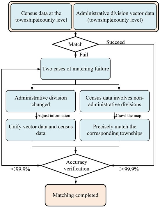
Figure 1. Workflow for matching census data with administrative boundaries.

2.2. A 100 m Gridded Population Dataset of China’s Seventh Census

The PopSE, developed by Chen et al. (2024) [9], was generated using a stacked ensemble model comprising Random Forest, LightGBM, and XGBoost. The PopSE dataset utilizes population statistics from partial county (The number of units at the county level is 2848) and township (The number of units at the township level is 15,564) levels of the 7th National Population Census as the dependent variable, along with a range of geospatial variables—including Tencent user location density, which reflects the spatial distribution of Tencent users based on location data from mobile applications like WeChat and QQ, and other variables such as points of interest (POI), nighttime lights, road density, digital elevation model (DEM), latitude/longitude, and building height—used as independent variables. In their modeling process, pixels where all of the following six auxiliary variables—Tencent user density, POI density, road density, nighttime lights, building height, and built-up area percentage—are equal to zero were designated as “uninhabited”. These “uninhabited” pixels are represented as “nodata” in PopSE. Therefore, the pixels that are marked as “nodata” in PopSE correspond to the areas that have been masked out, which can be treated as uninhabited regions. This dataset has been published and open access [31]. Therefore, we used PopSE as the habitable-area mask (hereafter referred to as the “habitable-area mask”), effectively masking out the remaining independent variables that represent non-residential areas. In addition, we also applied township-level dasymetric mapping to adjust the PopSE results (hereafter referred to as “adj_PopSE”), and used adj_PopSE as the independent variable in our models.

2.3. WorldPop’s Gridded Demographic Dataset

WorldPop’s Global 2015–2030 gridded demographic datasets (R2025A version v1, hereafter referred to as the “WorldPop”), launched in 2025, produce 100 m gridded population surfaces for 2015–2030 by training a Random-Forest–based weighting layer and redistributing census counts to grid cells via dasymetric mapping [30]. The latest release incorporates China’s 2020 county-level census, reducing biases introduced by outdated enumerations and growth-rate extrapolations. The WorldPop products provide 100 m estimates disaggregated by sex and five-year age groups (including <1 year). Because our analysis targets age-stratified spatial distributions—and prior evaluations for China indicate that WorldPop outperforms GPW3, GRUMP, and CnPop, remaining the best-performing product [35,36]—we adopt WorldPop as the reference dataset [7].

The latest WorldPop dataset provides three gender categories: “m” (male), “f” (female), and “t” (both male and female). For the purpose of generating a comparison dataset, we selected the “t” gender data. The specific process and data used are as follows (the full filename format is chn_t_xx_2020_CN_100 m_R2025A_v1; for convenience, the term “filename” below refers to the “xx” part of the full filename). The meaning of the filename is as follows: 00 refers to the population under 1 year of age, 01 to the population aged 1–4 years, 05 to the population aged 5–9 years, 90 to the population over 90 years old, and other filenames follow the same pattern as the 05 filename, representing the population in the respective age range. For the 0–14 years age group, we selected the datasets with filenames 00, 01, 05, and 10, and used the Raster Calculator to sum them and generate the comparison dataset for this age group. For the 15–59 years age group, we selected the datasets with filenames 15, 20, 25, 30, 35, 40, 45, 50, and 55, with the same calculation method and tool. For the 60–64 years age group, we selected the dataset with the filename 60. For the ≥65 years age group, we summed the remaining datasets.

2.4. Road Networks

Road networks are fundamental infrastructure for human activity and socio-economic exchange. Proximity to roads typically indicates greater transport accessibility and service availability. Accordingly, we derived a pixel-level road-accessibility metric defined as the Euclidean distance from the centroid of each 100 m grid cell to the nearest road segment, which was used as a model covariate. We sourced China’s 2020 road data from OpenStreetMap (OSM, accessed on 24 August 2025). As a widely used volunteered geographic information (VGI) platform, OSM has demonstrated high positional accuracy and completeness in prior studies [37,38,39] and is commonly—and effectively—used in population spatialization [8,40]. We computed nearest-distance surfaces and applied the habitable-area mask to limit noise from uninhabited areas, yielding a 100 m road-accessibility raster. It is important to note that the roads used in this study primarily include city roads, as well as provincial, county, and township-level roads, while excluding railways and expressways. Note that the roads used in this study primarily consisted of China’s first to fourth-level road networks, including Primary roads, Secondary roads, Tertiary roads, and Minor roads, while excluding railways and expressways.

2.5. POIs

Points of Interest (POIs) provide fine-grained, direct indicators of human activity and residential functions [19,21,41]. We programmatically retrieved 2020 POI data from Amap (https://www.amap.com/ (accessed on 24 August 2025)), China’s leading digital mapping and Location-Based Services (LBS) provider, excluding data from Hong Kong, Macau, and Taiwan. Each record includes geographic coordinates and a name-category-subcategory triplet. After cleaning and removing duplicates, we identified the top ten POI categories with the strongest empirical associations for each age group (see Section 3.1). These categories were then aggregated into four age group-specific POI datasets through weighted calculations, reflecting the total POI data for each group. The resulting age-stratified composite POI variables were used as one of the independent variables in the modeling process for generating ASPOP.

2.6. Remote Sensing Datasets

Gridded auxiliary data are indispensable inputs for population mapping and a key lever for improving accuracy and spatial fidelity. The widespread use of remote-sensing rasters in recent years has markedly enhanced the precision and robustness of population spatialization. Empirical evidence shows that judicious selection and fusion of multi-source gridded variables effectively capture spatial heterogeneity in population distributions [42,43,44]. Nighttime lights (NTL) serve as an effective proxy for human activity and are widely used in gridded population studies. We employed the 1 km NTL product from the NNU GeoData Yangtze River Delta Science Data Center, which fuses DMSP-OLS and SNPP-VIIRS via an extended cross-sensor calibration; the product reports high consistency at both pixel and city scales (R² ≈ 0.94), conferring advantages in spatial accuracy and temporal harmonization over the native sensors [32]. Consistent with WorldPop and related studies [18], elevation and slope were included as environmental variables, together with NTL, as independent variables in the model after applying the habitable-area mask [33].

3. Methods

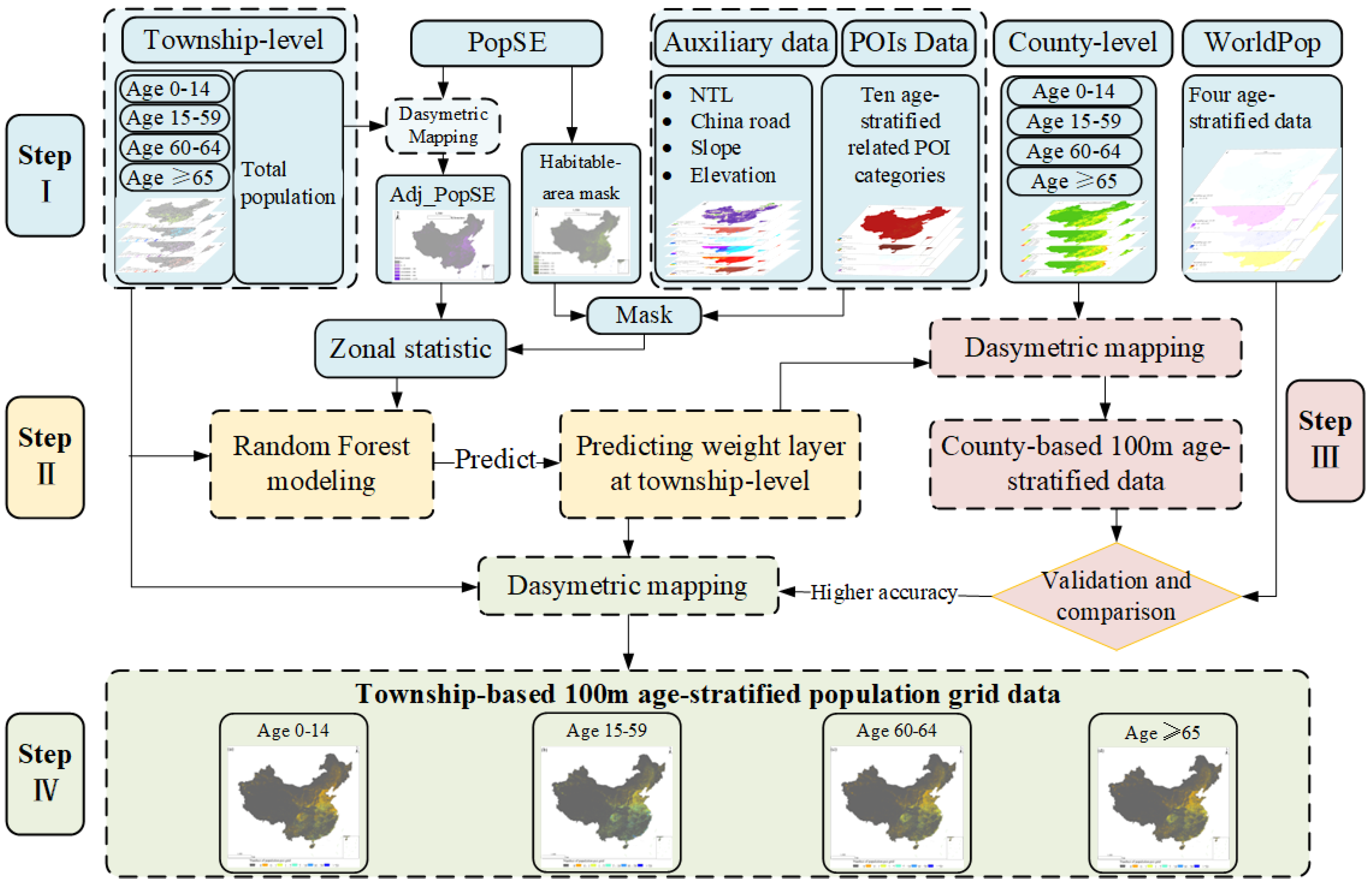
We developed an age-stratified downscaling approach by integrating a random forest model with age-filtered Points of Interest (POI) data and other multi-source geospatial covariates. The workflow comprises four main stages (Figure 2), as follows:

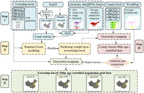
Figure 2. Flowchart of ASPOP generation and accuracy comparison process. Steps I–IV denote data collection and preprocessing, generation of age-stratified population density weighting layers, data comparison and validation, and final gridded population data production, respectively.

Data collection and preprocessing: Following the collection of census data and auxiliary variables, a series of preprocessing steps was performed. POI data were filtered by age group and subjected to kernel density analysis to convert point-based data into a gridded format. National road network data were used for Euclidean distance analysis to generate road accessibility rasters.

Generating Age-Stratified Population Density Weighting Layers: Age-stratified POI data, along with other covariates, were used to create four independent datasets. Separate random forest models were trained for each specific age stratum to predict and generate the age-stratified 100 m resolution population density weighting layers.

Data Comparison and Validation: As township-level data represent the finest publicly available spatial unit for demographic statistics in China, we further validated the accuracy by generating County-based 100 m Age-Stratified Population Grid Data (County-ASPOP) through dasymetric mapping using county-level age-stratified population counts. Both County-ASPOP and WorldPop data were aggregated to the township level to evaluate and compare the performance of the age-stratified population estimates.

Generating Stratified Population Grids: The final version of the age-stratified gridded population data was produced by applying dasymetric mapping to township-level census counts, using the population density weighting layers generated in the previous step.

3.1. Age-Stratified Screening of POI Categories

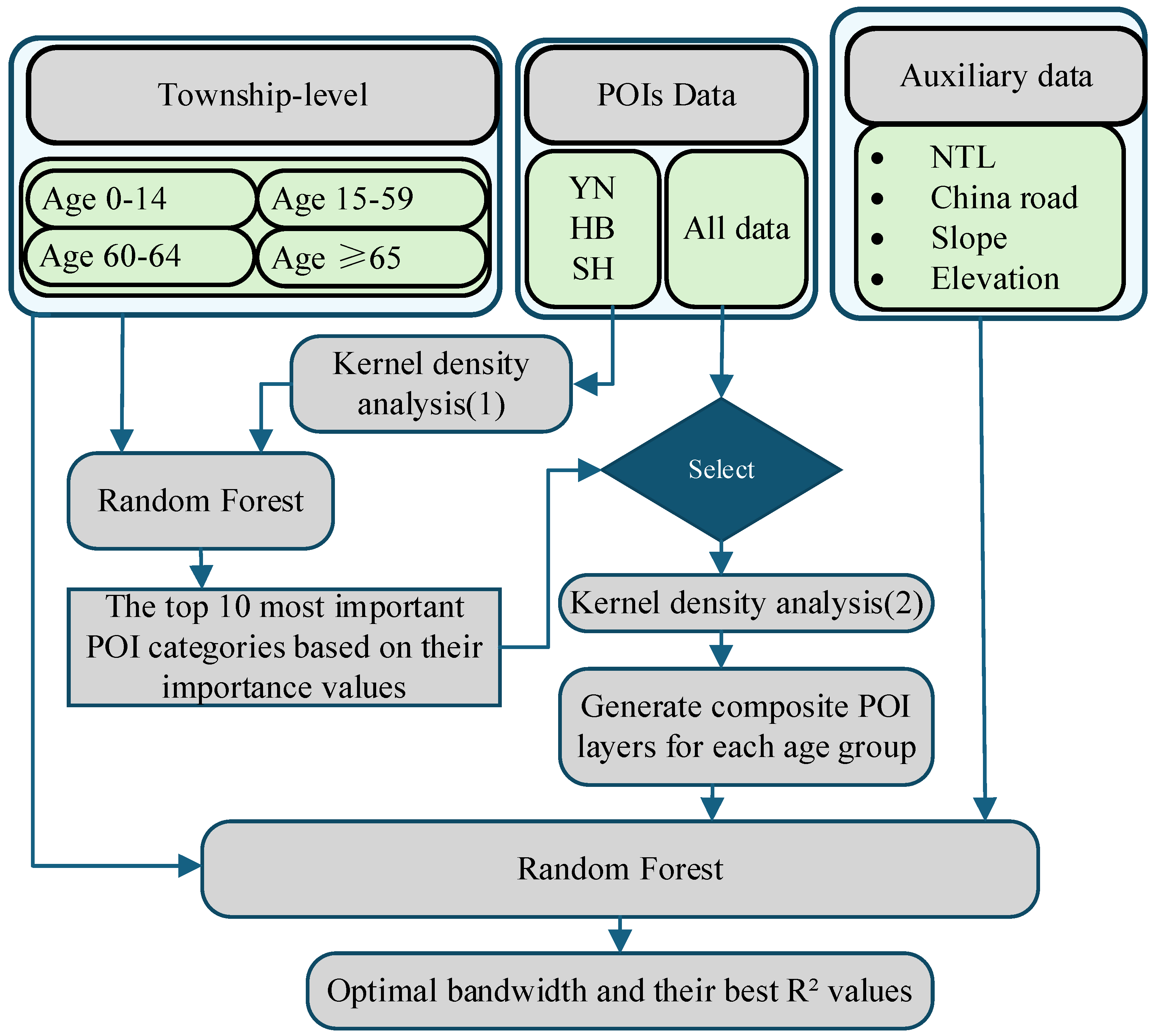
Evidence suggests that the explanatory power of Points of Interest (POI) for population density varies significantly across different age groups and density intervals, and simply increasing the number of POI categories does not necessarily improve model performance. Therefore, targeted screening of POI categories is necessary [45]. To identify the most explanatory POI types for each age group, we designed a novel experimental procedure (Figure 3). Prior to the experiment, we first cleaned the national POI dataset by removing invalid records, such as entries with missing names or categories, as well as data weakly associated with population distribution (e.g., “natural landmarks” and “highway toll stations”).

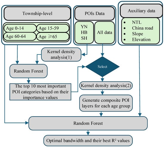
Figure 3. Age-stratified POI category selection process and determination of optimal bandwidth. In this picture, YN, SH, and HB represent Yunnan, Shanghai, and Hubei, respectively.

Firstly, the initial Screening of POI Categories. Three regions representative of China’s population density gradient—Shanghai (high density), Hubei (medium density), and Yunnan (low density)—were selected to reflect national population distribution characteristics. Kernel density analysis (bandwidth: 1 km, resolution: 100 m) was performed on the POI data from these regions, and the results were aggregated to the township level. The kernel density values of each POI category were used as independent variables to construct Random Forest (RF) models for each age group. It should be noted that the RF models in this step were not used to generate age-stratified population data, but specifically to identify the top 10 POI categories with the greatest explanatory power for the population distribution of each age group. After model training, the importance of each POI category was evaluated based on the %IncMSE metric, summarized and averaged across the three provinces, ultimately determining the 10 most explanatory POI categories for each age group. For example, the %IncMSE values of POI categories for the 0–14 age group in Shanghai, Hubei, and Yunnan were averaged, and the 10 categories with the highest average values were selected as representative POIs for the national 0–14 age group.

Secondly, bandwidth Optimization and Composite POI Layer Generation. For the top 10 POI categories selected for each age group, Kernel Density Estimation (KDE) raster layers at 100 m resolution were generated using fixed bandwidths of 1 km, 2 km, and 3 km. After applying a settlement mask to exclude non-residential areas, the results were aggregated to the township level and used as independent variables for subsequent RF models. The dependent variable was the natural logarithm of township-level population density for the corresponding age group. This step involved only POI kernel density layers and population data. Using the %IncMSE values of each POI category obtained from RF model training as weights (Table 2), the weighted formula (1) and (2) was applied via the Raster Calculator tool in ArcMap 10.8 to generate composite POI layers for each age group under the three bandwidths, which were used for optimal bandwidth selection in the next step.

Table 2. The weights of POI categories.

POI Categories	0–14	15–59	60–64	≥65
gli	0.05	0.12	0.20	0.23
giso	0.05	0.33	0.02	0.02
hs	0.11	0.04	0.19	0.17
fis	0.01	—	—	—
sls	0.34	0.17	0.19	0.19
pf	0.07	0.04	0.15	0.14
sshs	—	—	0.05	0.06
dls	—	0.07	—	—
rs	0.14	0.09	0.13	0.11
secs	0.22	—	—	—
ms	0.01	—	0.01	0.01
as	0.01	0.01	—	—
acs	—	0.04	—	—
ars	—	—	0.01	0.01
aus	—	—	0.06	0.07
br	—	0.09	—	—

Abbreviations: gli: Geographical Location Information; giso: Government Institutions and Social Organizations; hs: Healthcare Services; fis: Financial and Insurance Services; sls: Sports and Leisure Services; pf: Public Facilities; sshs: Scenic Spots and Historical Sites; dls: Daily Life Services; rs: Retail and Shopping Services; secs: Scientific, Educational, and Cultural Services; ms: Motorcycle Services; as: Automobile Sales; acs: Accommodation Services; ars: Automobile Maintenance and Repair; aus: Automotive Services; br: Commercial and Residential Properties.

Becides, determination of optimal bandwidth the composite POI layers for each age group under the three bandwidths (1 km, 2 km, and 3 km), along with other covariates such as slope and nighttime light data, were aggregated to the township level and used as independent variables in RF models, with the natural logarithm of township population density as the dependent variable. The data were split into 80% training and 20% testing sets, and RF models were trained for each age group, resulting in 12 models (3 bandwidths × 4 age groups). The optimal bandwidth for each age group was determined based on the R² values obtained from the testing set.

Among all age groups, the model with the 1 km bandwidth performed best, with R² values of 0.97 (0–14 years), 0.99 (15–59 years), 0.96 (60–64 years), and 0.96 (≥65 years) (Table 3). Notably, the preferred POI categories for the 60–64 and ≥65 age groups were highly consistent. This completes the process of screening key POI categories and determining the optimal bandwidth for each age group.

$$W_{t,i}={\displaystyle \frac{{\%IncMSE}_{t,i}}{{\sum }_{k=1}^{10}{\%IncMSE}_{t,k}}},\sum _{i=1}^{10}{W}_{t,i}=1,$$

(1)

$${POI}_t=\sum _{i=1}^{10}{W}_{t,i}{POI}_{t,i}$$

(2)

where $i=1\dots \dots 10$ indexes the ten POI categories and $t\in \{1,2,3,4\}$ denotes the age groups (0–14, 15–59, 60–64, ≥65); %${IncMSE}_{t,i}$ is the permutation importance (percent increase in OOB MSE) for category $i$ from the age-stratified random-forest model; ${POI}_{t,i}$ is the category-specific kernel-density covariate (100 m resolution; settlement mask applied); and ${POI}_t$ is the age-group composite POI covariate.

Table 3. Performance of age-stratified models under different bandwidths.

Age Group	1 km	2 km	3 km
0–14	0.97	0.97	0.97
15–59	0.99	0.99	0.99
60–64	0.96	0.96	0.96
≥65	0.96	0.96	0.96

3.2. Generating Age-Stratified Population Density Weighting Layers Using a Random Forest Model and the Application of Dasymetric Mapping

Random Forest (RF), introduced by Breiman in 2001 [46], is a non-parametric ensemble modeling technique. It constructs multiple sub-models by randomly selecting variables within classification and regression trees, and generates the final output through an automatic aggregation process, thereby improving the model’s generalization ability. Previous studies have shown that taking the natural logarithm of population density before modeling with RF can continuously improve the accuracy of aggregated prediction validation [47].

In our modeling process, we utilized the scikit-learn Python library to construct the RF model and employed a five-fold cross-validation strategy to enhance model robustness. For data partitioning, 80% of the township data was randomly selected for training models for the four age groups, with 20% reserved for model testing. For parameter optimization, we applied the BayesSearchCV method (from the skopt library) to conduct Bayesian parameter search, dynamically adjusting the RF parameters to achieve the best fit, with performance evaluated using R², RMSE, and MAE values on the test set. The best-performing model for each age group was used to predict the age-stratified population density weighting layer.

Subsequently, we applied Dasymetric Mapping to adjust the age-stratified population density weighting layers, redistributing the population from each source unit to target grid cells [47], ensuring volume conservation constraints [48]. Through township-level data dasymetric mapping, we produced the township-based 100 m Age-Stratified Population Grid Data (Township-ASPOP, Formula (3)). As township-level data represent the finest publicly available spatial unit for demographic statistics in China, we validated the accuracy by generating County-based 100 m Age-Stratified Population Grid Data (County-ASPOP) through distance-metric mapping using county-level age-stratified population counts (Formula (4)), as follows,

$${\mathrm{T}\mathrm{o}\mathrm{w}\mathrm{n}\mathrm{s}\mathrm{h}\mathrm{i}\mathrm{p}–\mathrm{A}\mathrm{S}\mathrm{P}\mathrm{O}\mathrm{P}}_i={\displaystyle \frac{{POP}_{township,i}}{{\sum }_{k=1}^N{W}_{i,k}}}\times W_{i,k},i=\left\{0–14, 15–59, 60–64, \ge 65\right\}$$

(3)

$${\mathrm{C}\mathrm{o}\mathrm{u}\mathrm{n}\mathrm{t}\mathrm{y}–\mathrm{A}\mathrm{S}\mathrm{P}\mathrm{O}\mathrm{P}}_i={\displaystyle \frac{{POP}_{county,i}}{{\sum }_{k=1}^N{W}_{i,k}}}\times W_{i,k},i=\left\{0–14, 15–59, 60–64, \ge 65\right\}$$

(4)

where ${\mathrm{C}\mathrm{o}\mathrm{u}\mathrm{n}\mathrm{t}\mathrm{y}–\mathrm{A}\mathrm{S}\mathrm{P}\mathrm{O}\mathrm{P}}_i$ and $\mathrm{T}\mathrm{o}\mathrm{w}\mathrm{n}\mathrm{s}\mathrm{h}\mathrm{i}\mathrm{p}–\mathrm{A}\mathrm{S}\mathrm{P}\mathrm{O}\mathrm{P}$ represent the estimated population for age group $i$ in a specific grid cell; ${POP}_{county,i}$ and ${POP}_{township,i}$ represent the total population for age group $i$ at the county-level and township-level; $W_{i,k}$ is the weight of grid cell $k$ for age group $i$, based on the prediction from the RF model; $N$ is the total number of pixels in the township; $i=\left\{0–14, 15–59, 60–64, \ge 65\right\}$ corresponds to the four age groups considered in the model.

3.3. Accuracy Evaluation

Since township-level census data and WorldPop [49] represent the most detailed available census and gridded population data, this study aggregates both WorldPop [49] and the County-ASPOP to the township level for further accuracy comparison. This approach is used to evaluate the performance of age-stratified gridded population data. Three metrics are employed to assess prediction accuracy: mean absolute error (MAE, (5), root mean square error (RMSE, (6), and the coefficient of determination (R², (7)):

$${MAE}_i={\displaystyle \frac{1}{N}}{\sum }_{k=1}^N\left|P_{i,k}-\widehat{P_{i,k}}\right|$$

(5)

$${RMSE}_i=\sqrt{\left({\displaystyle \frac{1}{N}}{\sum }_{k=1}^N{\left(P_{i,k}-\widehat{P_{i,k}}\right)}^2\right)}$$

(6)

$${R^2}_i=1-{\displaystyle \frac{{\sum }_{k=1}^N{\left(P_{i,k}-\widehat{P_{i,k}}\right)}^2}{{\sum }_{k=1}^N{\left(P_{i,k}-\overline{P_i}\right)}^2}}$$

(7)

$$i=\left\{0–14,15–59,60–64,\ge 65\right\}$$

where ${MAE}_i$ represents the Mean Absolute Error for age group $i$, measuring the average absolute difference between the predicted and observed population; ${RMSE}_i$ represents the Root Mean Square Error for age group $i$, which measures the square root of the average squared differences between the predicted and observed values, emphasizing larger errors; ${R^2}_i$ represents the Coefficient of Determination for age group $i$, indicating the proportion of variance in the observed data that is explained by the model, reflecting the goodness of fit; $N$ represents the total number of pixels in each county (i.e., the total number of grid cells used in the calculation); $P_{i,k}$ represents the observed population for age group $i$ in grid cell $k$; $\widehat{P_{i,k}}$ represents the predicted population for age group $i$ in grid cell $k$; $\overline{P_i}$ represents the average population for age group $i$ across all grid cells; and $i=\left\{0–14,15–59,60–64,\ge 65\right\}$ denotes the four age groups: 0–14 years, 15–59 years, 60–64 years, and ≥65 years.

4. Results

4.1. Model Evaluation

Table 4 presents the optimal parameters and goodness-of-fit evaluation results for the models across different age groups. The results indicate that all four age group models achieved an R² value greater than 0.95 on the test set, demonstrating strong performance in both model fitting and generalization. Among these, the model for the 15–59 age group performed the best, with an R² of 0.99, and RMSE and MAE values of 0.08 and 0.06, respectively. The models for the 0–14, 60–64, and ≥65 age groups showed similar accuracy, with R² values of 0.97, 0.96, and 0.96, respectively. For the 0–14 age group, the RMSE and MAE were 0.24 and 0.16, while for the 60–64 age group, they were 0.22 and 0.16. The model for the ≥65 age group exhibited relatively lower accuracy, with an R² of 0.96, and RMSE and MAE values of 0.24 and 0.17, respectively, representing the highest errors among the four age groups.

Table 4. Age-stratified models and their accuracy evaluation metrics on the population set.

Age-Stratified Models	R2	RMSE	MAE
0–14_RF	0.97	0.24	0.16
15–59_RF	0.99	0.08	0.06
60–64_RF	0.96	0.22	0.16
≥65_RF	0.96	0.24	0.17

4.2. Accuracy Assessment of New Maps

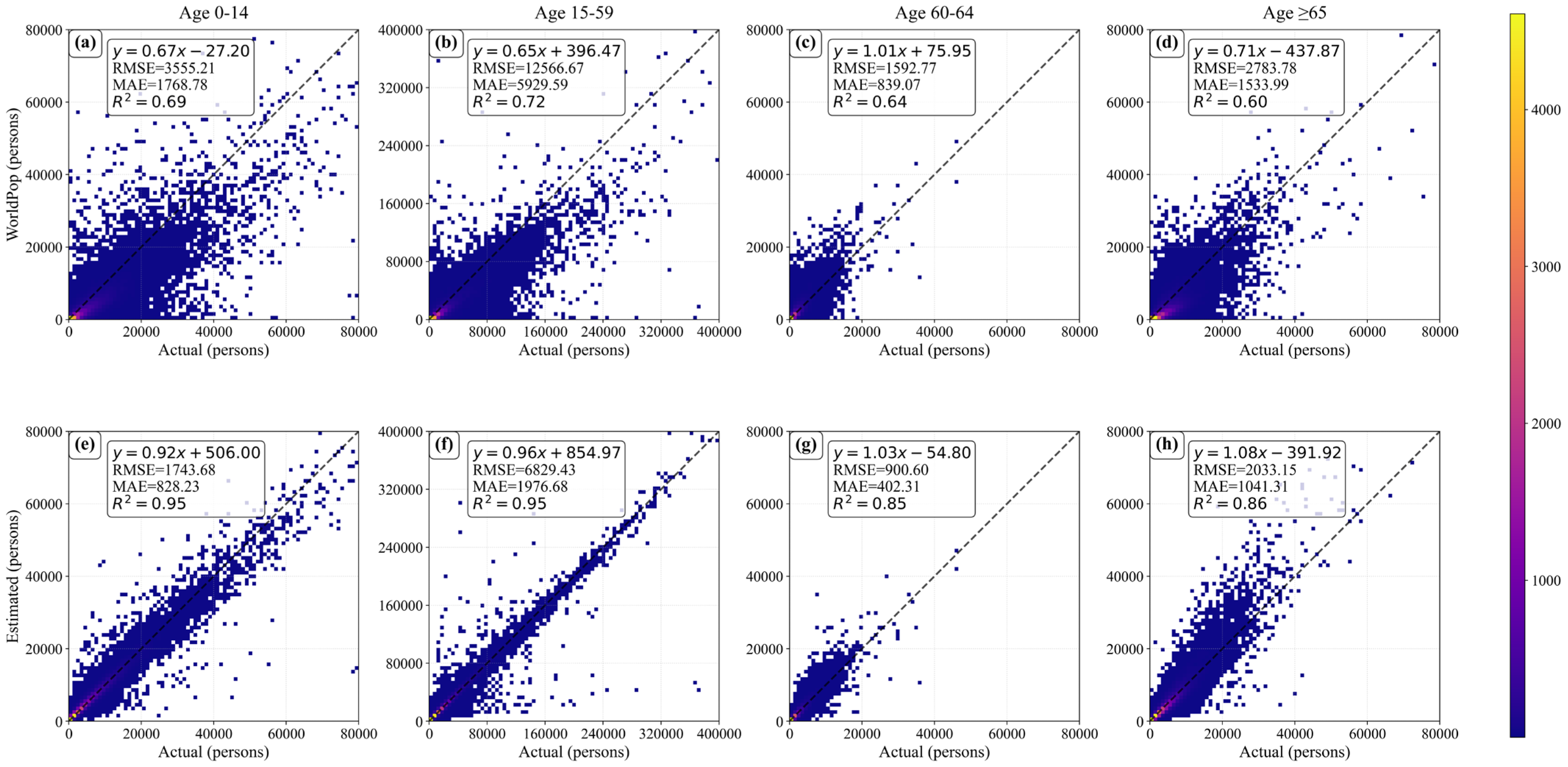
Figure 4 presents scatter plots of County-ASPOP at the township scale, after applying dasymetric mapping for calibration of the weight layers at the county level, alongside WorldPop data at the same scale. For the 0–14 years age group, the County-ASPOP significantly outperforms WorldPop across all metrics, indicating a substantial reduction in error and a marked enhancement in model fitting capability. The 15–59 years age group, representing the best-performing group, achieved an R² of 0.95, far exceeding WorldPop’s 0.72, with a regression slope of 0.96, indicating nearly an ideal fit. Although the larger population base for this age group resulted in relatively higher MAE (1976.68) and RMSE (6829.43), these values were still significantly better than WorldPop (MAE = 5929.59, RMSE = 125,66.67), demonstrating the model’s strong generalization ability and accuracy advantages. For the 60–64 years age group, the model’s performance was somewhat weaker, with an R² of 0.85, MAE of 402.31, and RMSE of 900.60. However, it still outperformed WorldPop (R² = 0.64, MAE = 839.07, RMSE = 1592.77). In the ≥65 years age group, the model yielded an R² of 0.86, with MAE and RMSE values of 1041.31 and 2033.15, respectively. The model’s goodness of fit was slightly lower compared to other age groups, but it still showed clear advantages over WorldPop (R² = 0.60, MAE = 1533.99, RMSE = 2783.78). The regression slope of 1.08 suggests a slight overestimation.

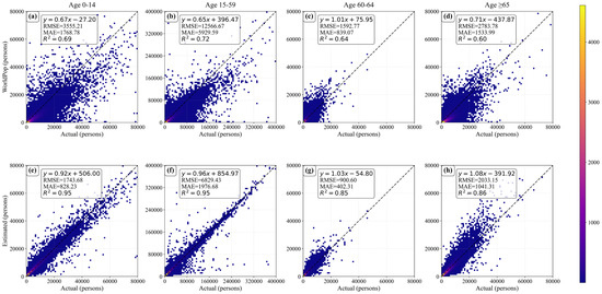
Figure 4. Accuracy comparison at the township scale: County-ASPOP versus WorldPop. (a–d) represent the accuracy of WorldPop at the township level, while (e–h) represent the accuracy of the County-ASPOP at the township level. Specifically, (a,e) correspond to the 0–14 age group, (b,f) correspond to the 15–59 age group, (c,g) correspond to the 60–64 age group, and (d,h) correspond to the ≥65 age group.

In summary, the County-ASPOP dataset demonstrates higher estimation accuracy compared to the WorldPop dataset, particularly for the 0–14 and 15–59 age groups. This improvement is primarily attributed to the enhanced spatial resolution of the model input data: our study employs township-level units as inputs, which represent the finest publicly available demographic units in China and enable a more precise depiction of population distribution details. Building upon the same weighting layer, our study further integrates township-level census data and applies dasymetric mapping to generate the high-accuracy Township-ASPOP dataset (Figure 5). By leveraging more detailed spatial information at the township level, Township-ASPOP is theoretically capable of capturing finer spatial distribution patterns of population across age groups. As a result, its accuracy is expected to be no less than that of County-ASPOP, with potential for further improvement.

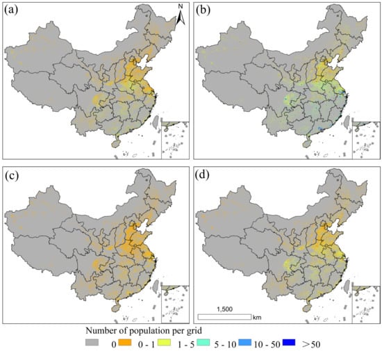
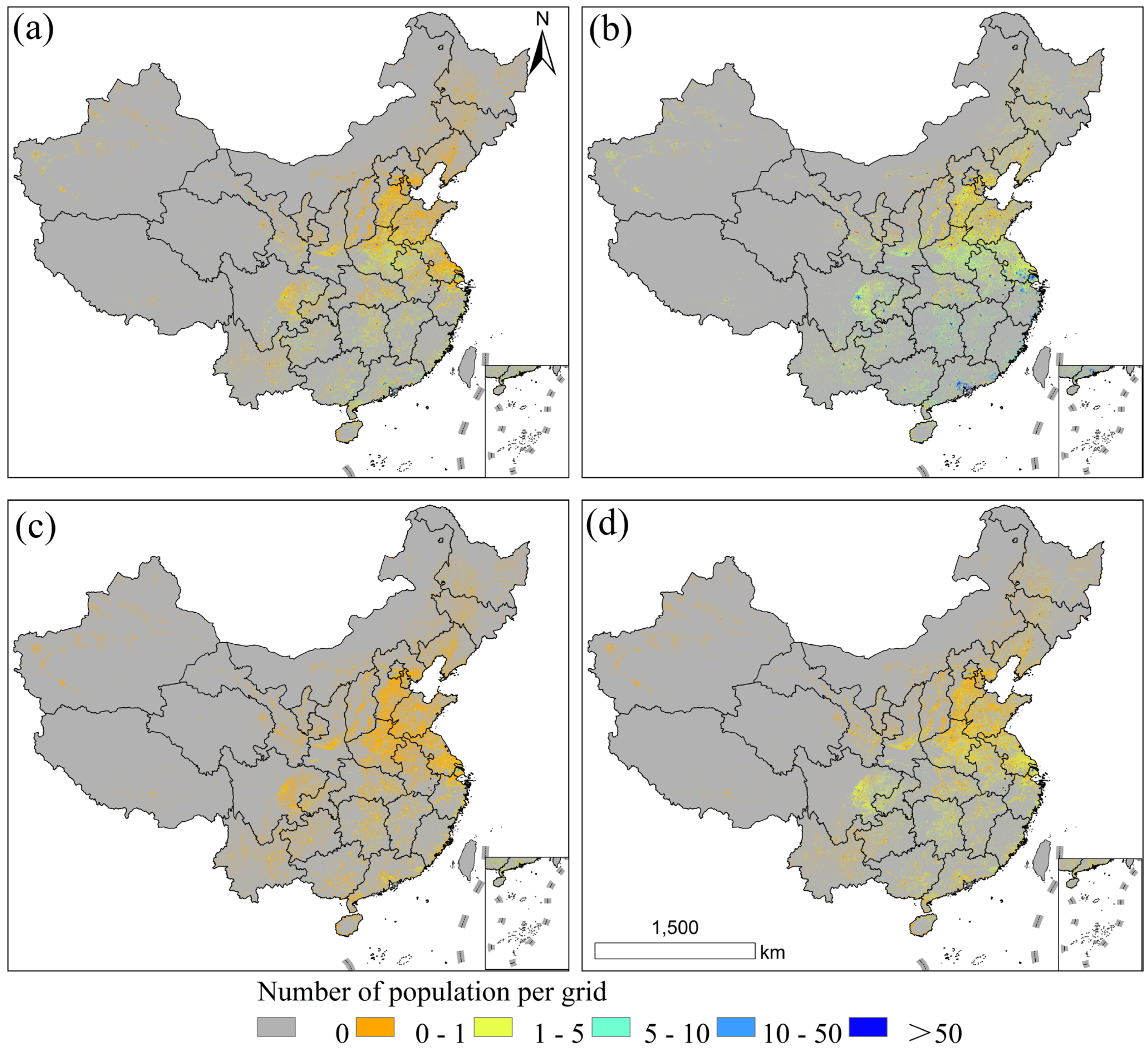
Figure 5. The Township-ASPOP for 0–14 years (a), 15–59 years (b), 60–64 years (c), ≥65 years (d).

Figure 5 presents the spatial distribution of the age-stratified population based on the Township-ASPOP dataset, with uninhabited areas shown in gray. Overall, populations across all age groups are concentrated in eastern coastal regions of China, including major population agglomerations such as the North China Plain, the Northeast China Plain, the Sichuan Basin, and the middle-lower reaches of the Yangtze River and Pearl River basins. Among these, the spatial clustering of the 15–59 age group is particularly pronounced. This gridded population distribution pattern intuitively aligns with the fundamental understanding of China’s demographic layout, visually affirming the effectiveness of the modeling approach proposed in this study.

4.3. Feature Importance of Age-Stratified Models

To investigate the differences in the contributions of variables in the age-stratified models, this study systematically analyzed the feature importance for the four age-stratified models based on the “feature_importances_” attribute of the RF model (Figure 6).

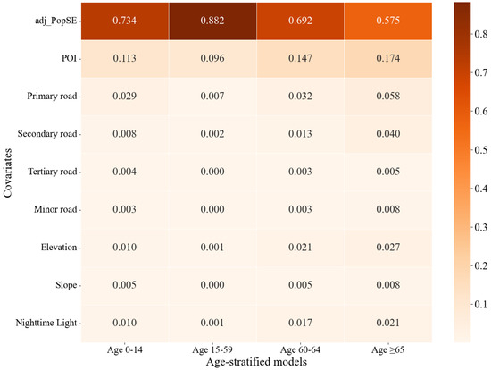
Figure 6. Variables’ importance for age-stratified models.

Overall, this study assumes that adj_PopSE is reasonable and incorporates it as one of the variables in the model training. Actually, the adj_PopSE shows exceptionally high importance across all four models, with its significance greatly surpassing that of the other variables. This indicates that the total population variable is highly representative in revealing the overall spatial distribution patterns of age-stratified populations, making it particularly suitable as prior data for spatial downscaling modeling. The R² values for total population and age-stratified populations are shown in Table 5, where it is evident that the total population is highly correlated with each age group.

Table 5. The relationship between the total population and age-stratified populations.

Age Group	County-Level R2	Township-Level R2
0–14	0.914	0.875
15–59	0.989	0.986
≥60	0.921	0.746
≥65	0.910	0.705

Among the secondary features, the POI kernel density variable for each age group ranked second in importance, further validating the effectiveness and relevance of POI data in reflecting the spatial activities of different populations. This result also demonstrates that the age-stratified POI variables developed in this study effectively capture the spatial heterogeneity of population age structures, providing crucial support for subsequent high-precision population mapping.

The importance of road network variables should also not be overlooked. The primary road variable ranked third for the four age groups. The secondary road variable also showed high importance in several models, highlighting that transportation accessibility significantly impacts the distribution of specific populations, especially the working-age and elderly groups.

Additionally, natural environmental variables such as elevation and slope exhibited relatively low importance across all four models. This may be attributed to the fact that the study area’s population is mainly concentrated in built-up and urban areas, where the spatial variability of natural factors is weaker, making it less effective in determining population distribution and thus reducing the model’s reliance on these variables. Nighttime lights were positioned in the middle range, showing a notable correlation with population distribution.

5. Discussion

5.1. Comparison of Age-Stratified Gridded Population Data for China in 2020

To explore population distribution patterns under different population density contexts, we selected three typical cities—Shanghai (high density), Linyi (medium density), and Lanzhou (low density)—and compared the Township-ASPOP and WorldPop datasets (Figure 7). The study found that the overall patterns of the two datasets are similar. In high-density Shanghai, the population distribution exhibits a significant central clustering pattern [50]. The population aged 0–14 is highly concentrated in the central urban areas, reflecting the strong appeal of high-quality educational and medical resources [23]. The working-age population (15–59 years) shows a coexistence of “core clustering and peripheral dispersion,” where employment opportunities attract population concentration toward the center, while living costs drive dispersal to the suburbs. The elderly population (60 years and above) remains notably concentrated in the central urban areas, forming a pattern of “urban concentration and suburban deep aging” [51]. The fundamental driving force behind this distribution lies in the significant disparities in key resources such as employment, education, and healthcare between central and peripheral areas [26,45]. In medium-density Linyi, a well-developed transportation network and a market-driven economy have promoted a polycentric development pattern. The population is not only concentrated in the main urban area but also widely distributed along county centers adjacent to major transportation routes, leading to a relative narrowing of the urban-rural gap [52,53]. Under this balanced framework, the spatial distribution patterns of different age groups tend to converge. In low-density Lanzhou, which is constrained by topography, resources are primarily concentrated in the southern river valley, resulting in an overall sparse population distribution but localized ribbon-like clustering along major transportation routes [54,55,56]. Due to fundamental constraints in resources and transportation conditions, all age groups follow this distribution pattern, with minimal differences among demographic segments.

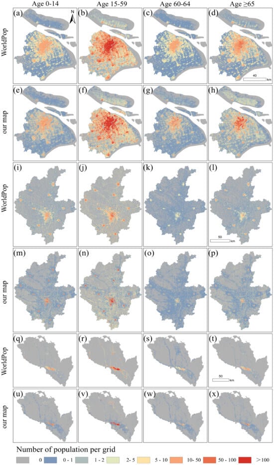
Figure 7. Comparison of population spatial distribution between WorldPop and the Township-ASPOP in cities with high (Shanghai), medium (Linyi), and low (Lanzhou) population densities. Panels (a–h) represent cities with high population density, (i–p) represent cities with medium population density, and (q–x) represent cities with low population density.

To thoroughly evaluate the applicability of different population datasets in refined decision-making, this study spatially subtracted the Township-ASPOP and WorldPop datasets, revealing their respective biases in depicting the spatial distribution of different age groups (Figure 8). Analysis indicates these discrepancies exhibit distinct spatial patterns and age-group specificity: In urban core areas, Township-ASPOP estimates consistently exceed WorldPop across all age groups, with the most pronounced differences observed in the 0–14 and 15–59 age cohorts. This reflects Township-ASPOP’s superior ability to capture the attractiveness of public services such as education and employment. This discrepancy stems from differences in modeling methodologies and input data precision [57]. Township-ASPOP, grounded in finer-grained localized data, more sensitively reflects the clustering effects driven by diverse needs—such as schooling and employment—across age groups [58,59]. Conversely, the WorldPop model tends to produce smoothing effects that may obscure spatial differentiation between age cohorts. This implies that data selection directly impacts age-structured public policies. For instance, when planning schools or elderly care facilities, using data that underestimates the number of children or working-age individuals may lead to an underestimation of actual service needs in core urban areas, resulting in imbalanced resource allocation [60,61,62,63]. In emergency management, if data used to assess risk-exposed populations fails to accurately distinguish age groups with different disaster resilience levels, it can severely compromise the precision of evacuation and rescue plans [5,60,64]. Therefore, despite similar macro-level patterns, these differences caution us that dataset selection impacts policy targeting. Utilizing localized datasets that better reflect the spatial details of population age structures holds significant value for urban planning and precise social risk management [65,66].

5.2. Advantage

This study offers several key advantages over previous research. First, it uses the latest and most detailed 2020 China township-level census data, which includes a total of 38,572 township-level data entries. This is a significant advantage over prior studies, which typically rely on county-level data or county-township mixed-scale data [9,21,27]. Township-level data provides much higher spatial resolution, enabling a more precise representation of population distribution patterns and significantly improving model prediction accuracy. Additionally, we integrated a variety of heterogeneous, multi-source data as variables, including POI, terrain factors (elevation and slope), and nighttime lights. This comprehensive integration of data resulted in better model performance compared to existing age-stratified population datasets, such as WorldPop, which do not offer the same level of granularity or accuracy at the township level.

Second, by using the habitable-area mask, we excluded non-residential areas, which further enhanced the accuracy of population downscaling modeling. Many existing studies fail to effectively filter non-residential areas, which can lead to overestimation or misrepresentation of populations. In contrast, the masking strategy in this study effectively mitigates such errors.

Figure 8. Spatial distribution of population differences between the Township-ASPOP and WorldPop datasets for Shanghai (a–d), Linyi (e–h), and Lanzhou (i–l). For each city, the subpanels represent the age groups 0–14 (a,e,i), 15–59 (b,f,j), 60–64 (c,g,k), and ≥65 (d,h,l) years, respectively. Green indicates overestimation by WorldPop relative to Township-ASPOP, while red indicates underestimation.

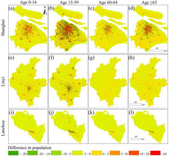
Figure 8. Spatial distribution of population differences between the Township-ASPOP and WorldPop datasets for Shanghai (a–d), Linyi (e–h), and Lanzhou (i–l). For each city, the subpanels represent the age groups 0–14 (a,e,i), 15–59 (b,f,j), 60–64 (c,g,k), and ≥65 (d,h,l) years, respectively. Green indicates overestimation by WorldPop relative to Township-ASPOP, while red indicates underestimation.

Finally, this study customizes variables based on the activity characteristics of different age groups, extracting age-stratified functional POI categories from the full POI dataset for modeling. For example, educational POIs are selected for the child population, industrial and enterprise POIs for the working-age population, and medical and elderly care POIs for the elderly. This population behavior-based customization of variables effectively addresses the issue of homogeneous variables often found in previous age-stratified population downscaling studies [23,34], significantly enhancing the model’s ability to respond to the distribution characteristics of different age groups.

Moreover, our approach to handling POI data is more refined than in other studies. Instead of using a single, unified POI layer, we conducted category selection and age-stratified differentiation to maximize model performance.

5.3. Limitations and Future Work

We developed an age-stratified downscaling framework to generate a high-accuracy 100 m resolution age-stratified population density data. Although our research has achieved good results, there are still some limitations. First, this study utilized the classical RF algorithm. Although this method is widely applied in geographic modeling and spatial prediction [9,21,47,67] and offers good robustness and interpretability, it still has limitations compared to more advanced machine learning and deep learning methods that have emerged in recent years (e.g., LightGBM, XGBoost, Graph Neural Networks, Convolutional Neural Networks) in handling complex nonlinear relationships and spatial heterogeneity. Future work could focus on improving model prediction accuracy through the use of advanced algorithms or multi-algorithm stacking. Second, data-related limitations present significant challenges. The quality and completeness of the Points of Interest (POI) data, while refined through age-stratified filtering, may still be uneven across regions, particularly in rural or underdeveloped areas, potentially leading to population underestimation. Furthermore, the integration of multi-source geospatial variables (e.g., nighttime lights, road networks) introduces challenges of scale mismatch and potential positional errors, which could propagate uncertainty into the model. Future research should, therefore, focus not only on algorithmic improvements but also on incorporating higher-fidelity and more frequently updated ancillary data. Exploring methods to quantify and mitigate the propagation of input data errors, as well as extending the framework to spatiotemporal modeling, will be the critical next steps.

6. Conclusions

This study, based on the 2020 China Seventh Population Census data, combines multi-source auxiliary variables to develop a downscaling model for age-stratified population data. The main innovations of this research are as follows: First, an age-stratified POI classification system was developed to address the characteristics of different age groups, and representative spatial variables were extracted accordingly. Second, a robust and interpretable RF model was employed for modeling, with hyperparameter optimization achieved through Bayesian optimization to enhance model prediction accuracy. Third, existing high-resolution residential area masks were introduced as spatial constraints, significantly improving prediction accuracy at the 100 m scale.

The experimental results show that the four age-stratified gridded population datasets constructed in this study outperform existing population grid datasets in both accuracy and spatial performance. Particularly in terms of accuracy, the model demonstrates higher fit and lower error compared to observed data at the township scale. Spatially, this study effectively addresses the overestimation in urban centers and underestimation in suburban areas observed in existing datasets.

In conclusion, this study provides a new methodological approach and data support for the high-resolution spatial representation of age-stratified populations in China. The resulting population data can offer more accurate foundations for resource allocation, public service planning, disaster risk assessment, and regional economic analysis.

References

- Zheng, Z. From the past to the future: What we learn from China’s 2020 Census. China Popul. Dev. Stud. 2021, 5, 101–106. [Google Scholar] [CrossRef]
- Luo, Y.; Su, B.; Zheng, X. Trends and Challenges for Population and Health During Population Aging—China, 2015–2050. China CDC Wkly. 2021, 3, 593–598. [Google Scholar] [CrossRef]
- Baynes, J.; Neale, A.; Hultgren, T. Improving intelligent dasymetric mapping population density estimates at 30 m resolution for the conterminous United States by excluding uninhabited areas. Earth Syst. Sci. Data 2022, 14, 2833–2849. [Google Scholar] [CrossRef]
- Gao, P.; Wu, T.; Ge, Y.; Li, Z. Improving the accuracy of extant gridded population maps using multisource map fusion. Gisci. Remote Sens. 2022, 59, 54–70. [Google Scholar] [CrossRef]
- Jing, R.; Heft-Neal, S.; Chavas, D.R.; Griswold, M.; Wang, Z.; Clark-Ginsberg, A.; Guha-Sapir, D.; Bendavid, E.; Wagner, Z. Global population profile of tropical cyclone exposure from 2002 to 2019. Nature 2024, 626, 549–554. [Google Scholar] [CrossRef] [PubMed]
- He, M.; Xu, Y.; Li, N. Population Spatialization in Beijing City Based on Machine Learning and Multisource Remote Sensing Data. Remote Sens. 2020, 12, 1910. [Google Scholar] [CrossRef]
- Lei, Z.; Xie, Y.; Cheng, P.; Yang, H. From auxiliary data to research prospects, a review of gridded population mapping. Trans. GIS 2023, 27, 3–39. [Google Scholar] [CrossRef]
- Ma, Y.; Zhou, C.; Li, M. A novel approach to improve population mapping considering facility-based service capacity and land livability. Int. J. Geogr. Inf. Sci. 2025, 39, 346–375. [Google Scholar] [CrossRef]
- Chen, Y.; Xu, C.; Ge, Y.; Zhang, X.; Zhou, Y. A 100 m gridded population dataset of China’s seventh census using ensemble learning and big geospatial data. Earth Syst. Sci. Data 2024, 16, 3705–3718. [Google Scholar] [CrossRef]
- Zhao, Y.; Zhang, Y.; Wang, H.; Du, X.; Li, Q.; Zhu, J. Intraday Variation Mapping of Population Age Structure via Urban-Functional-Region-Based Scaling. Remote Sens. 2021, 13, 805. [Google Scholar] [CrossRef]
- Wardrop, N.A.; Jochem, W.C.; Bird, T.J.; Chamberlain, H.R.; Clarke, D.; Kerr, D.; Bengtsson, L.; Juran, S.; Seaman, V.; Tatem, A.J. Spatially disaggregated population estimates in the absence of national population and housing census data. Proc. Natl. Acad. Sci. USA 2018, 115, 3529–3537. [Google Scholar] [CrossRef]
- Leyk, S.; Gaughan, A.E.; Adamo, S.B.; de Sherbinin, A.; Balk, D.; Freire, S.; Rose, A.; Stevens, F.R.; Blankespoor, B.; Frye, C.; et al. The spatial allocation of population: A review of large-scale gridded population data products and their fitness for use. Earth Syst. Sci. Data 2019, 11, 1385–1409. [Google Scholar] [CrossRef]
- Sadeghi, M.; Karimi, M.; Rabiei-Dastjerdi, H.; Sarkar, D. Multi-scale dynamic population estimation: An Adaptive Inverse Distance Weighting (AIDW) model incorporating spatial characteristics. Cartogr. Geogr. Inf. Sci. 2025, 53, 129–154. [Google Scholar] [CrossRef]
- Chen, Y.; Zhang, R.; Ge, Y.; Jin, Y.; Xia, Z. Downscaling Census Data for Gridded Population Mapping With Geographically Weighted Area-to-Point Regression Kriging. IEEE Access 2019, 7, 149132–149141. [Google Scholar] [CrossRef]
- Mennis, J.; Hultgren, T. Intelligent Dasymetric Mapping and Its Application to Areal Interpolation. Cartogr. Geogr. Inf. Sci. 2006, 33, 179–194. [Google Scholar] [CrossRef]
- Mennis, J. Generating Surface Models of Population Using Dasymetric Mapping. Prof. Geogr. 2003, 55, 31–42. [Google Scholar] [CrossRef]
- Wright, J.K. A Method of Mapping Densities of Population: With Cape Cod as an Example. Geogr. Rev. 1936, 26, 103. [Google Scholar] [CrossRef]
- Tatem, A.J. WorldPop, open data for spatial demography. Sci. Data 2017, 4, 170004. [Google Scholar] [CrossRef]
- Li, K.; Chen, Y.; Li, Y. The Random Forest-Based Method of Fine-Resolution Population Spatialization by Using the International Space Station Nighttime Photography and Social Sensing Data. Remote Sens. 2018, 10, 1650. [Google Scholar] [CrossRef]
- Wang, L.; Fan, H.; Wang, Y. Improving population mapping using Luojia 1-01 nighttime light image and location-based social media data. Sci. Total Environ. 2020, 730, 139148. [Google Scholar] [CrossRef]
- Ye, T.; Zhao, N.; Yang, X.; Ouyang, Z.; Liu, X.; Chen, Q.; Hu, K.; Yue, W.; Qi, J.; Li, Z.; et al. Improved population mapping for China using remotely sensed and points-of-interest data within a random forests model. Sci. Total Environ. 2019, 658, 936–946. [Google Scholar] [CrossRef]
- Li, L.; Zhang, Y.; Liu, L.; Wang, Z.; Zhang, H.; Li, S.; Ding, M. Mapping Changing Population Distribution on the Qinghai–Tibet Plateau since 2000 with Multi-Temporal Remote Sensing and Point-of-Interest Data. Remote Sens. 2020, 12, 4059. [Google Scholar] [CrossRef]
- Wang, W.; Pei, T.; Chen, J.; Song, C.; Wang, X.; Shu, H.; Ma, T.; Du, Y. Population Distributions of Age Groups and Their Influencing Factors Based on Mobile Phone Location Data: A Case Study of Beijing, China. Sustainability 2019, 11, 7033. [Google Scholar] [CrossRef]
- Thomson, D.R.; Rhoda, D.A.; Tatem, A.J.; Castro, M.C. Gridded population survey sampling: A systematic scoping review of the field and strategic research agenda. Int. J. Health Geogr. 2020, 19, 34. [Google Scholar] [CrossRef]
- Swanwick, R.H.; Read, Q.D.; Guinn, S.M.; Williamson, M.A.; Hondula, K.L.; Elmore, A.J. Dasymetric population mapping based on US census data and 30-m gridded estimates of impervious surface. Sci. Data 2022, 9, 523. [Google Scholar] [CrossRef] [PubMed]
- Zhao, S.; Liu, Y.; Zhang, R.; Fu, B. China’s population spatialization based on three machine learning models. J. Clean. Prod. 2020, 256, 120644. [Google Scholar] [CrossRef]
- Chen, M.; Xian, Y.; Huang, Y.; Zhang, X.; Hu, M.; Guo, S.; Chen, L.; Liang, L. Fine-scale population spatialization data of China in 2018 based on real location-based big data. Sci. Data 2022, 9, 624. [Google Scholar] [CrossRef]
- Xu, X.; Tan, M.; Liu, X.; Wang, X.; Xin, L. Stability and Changes in the Spatial Distribution of China’s Population in the Past 30 Years Based on Census Data Spatialization. Remote Sens. 2023, 15, 1674. [Google Scholar] [CrossRef]
- Man, W.; Wang, S.; Yang, H. Exploring the spatial-temporal distribution and evolution of population aging and social-economic indicators in China. BMC Public Health 2021, 21, 966. [Google Scholar] [CrossRef]
- Bondarenko, M.P.R.T.N. Estimates of 2015–2030 Total Number of People per Grid Square Broken Down by Gender and Age Groupings at a Resolution of 3 Arc (Approximately 100 m at the Equator) R2025A Version v1. 2025. Available online: https://hub.worldpop.org/project/categories?id=8 (accessed on 6 January 2026).
- Chen, Y.; Xu, C.; Ge, Y.; Zhang, X.; Zhou, Y. A 100-m gridded population dataset of China’s seventh census using ensemble learning and geospatial big data. Figshare 2024. [Google Scholar] [CrossRef]
- Wu, Y.; Shi, K.; Chen, Z.; Liu, S.; Chang, Z. Developing Improved Time-Series DMSP-OLS-Like Data (1992–2019) in China by Integrating DMSP-OLS and SNPP-VIIRS. IEEE Trans. Geosci. Remote Sens. 2022, 60, 1–14. [Google Scholar] [CrossRef]
- Farr, T.G.; Rosen, P.A.; Caro, E.; Crippen, R.; Duren, R.; Hensley, S.; Kobrick, M.; Paller, M.; Rodriguez, E.; Roth, L.; et al. The Shuttle Radar Topography Mission. Rev. Geophys. 2007, 45. [Google Scholar] [CrossRef]
- Ju, Y.; Liang, Y.; Kong, J.; Wang, X.; Wen, S.; Shang, H.; Wang, X. 100-m resolution Age-Stratified Population Estimation from the 2020 China Census by Township (ASPECT). Sci. Data 2025, 12, 1058. [Google Scholar] [CrossRef]
- Bai, Z.; Wang, J.; Wang, M.; Gao, M.; Sun, J. Accuracy Assessment of Multi-Source Gridded Population Distribution Datasets in China. Sustainability 2018, 10, 1363. [Google Scholar] [CrossRef]
- Xu, Y.; Ho, H.C.; Knudby, A.; He, M. Comparative assessment of gridded population data sets for complex topography: A study of Southwest China. Popul. Environ. 2020, 42, 360–378. [Google Scholar] [CrossRef]
- Borkowska, S.; Pokonieczny, K. Analysis of OpenStreetMap Data Quality for Selected Counties in Poland in Terms of Sustainable Development. Sustainability 2022, 14, 3728. [Google Scholar] [CrossRef]
- Wu, J.; Han, S.; Shi, L.; Hui, Q. Study on the spatial variability of thermal landscape in Xi’an based on OSM road network and POI data. Front. Ecol. Evol. 2023, 11. [Google Scholar] [CrossRef]
- Zhao, P.; Jia, T.; Qin, K.; Shan, J.; Jiao, C. Statistical analysis on the evolution of OpenStreetMap road networks in Beijing. Phys. A 2015, 420, 59–72. [Google Scholar] [CrossRef]
- Rosina, K.; Hurbánek, P.; Cebecauer, M. Using OpenStreetMap to improve population grids in Europe. Cartogr. Geogr. Inf. Sci. 2017, 44, 139–151. [Google Scholar] [CrossRef]
- Yang, X.; Ye, T.; Zhao, N.; Chen, Q.; Yue, W.; Qi, J.; Zeng, B.; Jia, P. Population Mapping with Multisensor Remote Sensing Images and Point-Of-Interest Data. Remote Sens. 2019, 11, 574. [Google Scholar] [CrossRef]
- Gaughan, A.E.; Stevens, F.R.; Huang, Z.; Nieves, J.J.; Sorichetta, A.; Lai, S.; Ye, X.; Linard, C.; Hornby, G.M.; Hay, S.I.; et al. Spatiotemporal patterns of population in mainland China, 1990 to 2010. Sci. Data 2016, 3, 160005. [Google Scholar] [CrossRef] [PubMed]
- McKeen, T.; Bondarenko, M.; Kerr, D.; Esch, T.; Marconcini, M.; Palacios-Lopez, D.; Zeidler, J.; Valle, R.C.; Juran, S.; Tatem, A.J.; et al. High-resolution gridded population datasets for Latin America and the Caribbean using official statistics. Sci. Data 2023, 10, 436. [Google Scholar] [CrossRef] [PubMed]
- Sinha, P.; Gaughan, A.E.; Stevens, F.R.; Nieves, J.J.; Sorichetta, A.; Tatem, A.J. Assessing the spatial sensitivity of a random forest model: Application in gridded population modeling. Comput. Environ. Urban Syst. 2019, 75, 132–145. [Google Scholar] [CrossRef]
- Huang, Y.; Lin, T.; Zhang, G.; Zhu, W.; Hamm, N.A.S.; Liu, Y.; Zhang, J.; Yao, X. Exploring the Relationship between the Spatial Distribution of Different Age Populations and Points of Interest (POI) in China. ISPRS Int. J. Geo-Inf. 2022, 11, 215. [Google Scholar] [CrossRef]
- Breiman, L. Random Forests. Mach. Learn. 2001, 45, 5–32. [Google Scholar] [CrossRef]
- Stevens, F.R.; Gaughan, A.E.; Linard, C.; Tatem, A.J. Disaggregating Census Data for Population Mapping Using Random Forests with Remotely-Sensed and Ancillary Data. PLoS ONE 2015, 10, e0107042. [Google Scholar] [CrossRef]
- Wang, L.; Wang, S.; Zhou, Y.; Liu, W.; Hou, Y.; Zhu, J.; Wang, F. Mapping population density in China between 1990 and 2010 using remote sensing. Remote Sens. Environ. 2018, 210, 269–281. [Google Scholar] [CrossRef]
- Bondarenko, M.; Kerr, D.; Sorichetta, A.; Tatem, A. Estimates of 2020 Total Number of People per Grid Square Broken Down by Gender and Age Groupings Using Built-Settlement Growth Model (BSGM) Outputs. University of Southampton. 2020. Available online: https://hub.worldpop.org/doi/10.5258/SOTON/WP00695 (accessed on 6 January 2026).
- Sun, L.; Zhu, K. The Social Dimension of Urban Transformation in Shanghai: Population Mobility, Modernity, and Globalization. J. Urban Hist. 2022, 48, 213–221. [Google Scholar] [CrossRef]
- Yang, Z.; Zhao, Q.; Jiang, P.; Zheng, S.; Xu, B. Prevalence and control of hypertension among a Community of Elderly Population in Changning District of shanghai: A cross-sectional study. BMC Geriatr. 2017, 17, 296. [Google Scholar] [CrossRef]
- Zhou, J.; Wu, Y. Study on the Optimal Urban Population Size under Multi-objective Decision-making: Take Linyi City as an Example. Value Eng. 2022, 160–162. [Google Scholar]
- Han, H.L.; Li, X.Z. Study on the Population Siphon Effect of the Main Urban Area of Linyi City. Ind. Sci. Trib. 2023, 22, 59–61. [Google Scholar] [CrossRef]
- Jia, Z.; Chen, X.; Li, C. Spatial pattern of population aggregation of Lanzhou-Xining urban agglomeration and its influence factors. J. Lanzhou Univ. (Nat. Sci. Ed.) 2019, 55, 436–442. [Google Scholar] [CrossRef]
- Zhang, X.H.; Zhang, N.; Wang, S.H. Spatial Agglomeration and Its Influencing Factors of Population in Western Valley City since 2000: A Case Study of Lanzhou City. Mod. Urban Res. 2025, 58–64. [Google Scholar]
- Zhang, Z.B.; Pan, J.; Da, F.W. Population spatial structure evolution pattern and regulating pathway in Lanzhou City. Geogr. Res. 2012, 31, 2055–2068. [Google Scholar]
- Yu, H.S.Y.K. Trends in social vulnerability to storm surges in Shenzhen, China. Nat. Hazards Earth Syst. Sci. 2020, 20, 2447–2462. [Google Scholar] [CrossRef]
- Yang, C.; Cui, D.; Yin, S.; Wu, R.; Ke, X.; Liu, X.; Yang, Y.; Sun, Y.; Xu, L.; Teng, C. Fiscal autonomy of subnational governments and equity in healthcare resource allocation: Evidence from China. Front. Public Health 2022, 10, 989625. [Google Scholar] [CrossRef]
- Wang, Y.; Liu, Y.; Xing, L.; Zhang, Z. An Improved Accessibility-Based Model to Evaluate Educational Equity: A Case Study in the City of Wuhan. ISPRS Int. J. Geo-Inf. 2021, 10, 458. [Google Scholar] [CrossRef]
- Liu, Y.; Lu, C.; Yang, X.; Wang, Z.; Liu, B. Fine-Scale Coastal Storm Surge Disaster Vulnerability and Risk Assessment Model: A Case Study of Laizhou Bay, China. Remote Sens. 2020, 12, 1301. [Google Scholar] [CrossRef]
- Hoxby, C.M. Does competition among public schools benefit students and taxpayers? Am. Econ. Rev. 2000, 90, 1209–1238. [Google Scholar] [CrossRef]
- Gong, J.; Wang, G.; Wang, Y.; Chen, X.; Chen, Y.; Meng, Q.; Yang, P.; Yao, Y.; Zhao, Y. Nowcasting and forecasting the care needs of the older population in China: Analysis of data from the China Health and Retirement Longitudinal Study (CHARLS). Lancet Public Health 2022, 7, e1005–e1013. [Google Scholar] [CrossRef]
- Chen, Y.; Feng, S. The education of migrant children in China’s urban public elementary schools: Evidence from Shanghai. China Econ. Rev. 2019, 54, 390–402. [Google Scholar] [CrossRef]
- Zeng, J.; Zhu, Z.Y.; Zhang, J.L.; Ouyang, T.P.; Qiu, S.F.; Zou, Y.; Zeng, T. Social vulnerability assessment of natural hazards on county-scale using high spatial resolution satellite imagery: A case study in the Luogang district of Guangzhou, South China. Environ. Earth Sci. 2012, 65, 173–182. [Google Scholar] [CrossRef]
- MacManus, K.; Balk, D.; Engin, H.; McGranahan, G.; Inman, R. Estimating population and urban areas at risk of coastal hazards, 1990–2015: How data choices matter. Earth. Syst. Sci. Data 2021, 13, 5747–5801. [Google Scholar] [CrossRef]
- Hanberry, B.B. Urban Land Expansion and Decreased Urban Sprawl at Global, National, and City Scales during 2000 to 2020. Ecosyst. Health Sustain. 2023, 9, 74. [Google Scholar] [CrossRef]
- Liu, L.; Chen, R.; Zhao, Q.; Zhu, S. Applying a multistage of input feature combination to random forest for improving MRT passenger flow prediction. J. Ambient. Intell. Humaniz. Comput. 2018, 10, 4515–4532. [Google Scholar] [CrossRef]
Disclaimer/Publisher’s Note: The statements, opinions and data contained in all publications are solely those of the individual author(s) and contributor(s) and not of MDPI and/or the editor(s). MDPI and/or the editor(s) disclaim responsibility for any injury to people or property resulting from any ideas, methods, instructions or products referred to in the content. |
© 2026 by the authors. Licensee MDPI, Basel, Switzerland. This article is an open access article distributed under the terms and conditions of the Creative Commons Attribution (CC BY) license.