VitralColor-12: A Synthetic Twelve-Color Segmentation Dataset from GPT-Generated Stained-Glass Images

Abstract

The segmentation and classification of color are crucial stages in image processing, computer vision, and pattern recognition, as they significantly impact the results. The diverse, hand-labeled datasets in the literature are applied for monochromatic or color segmentation in specific domains. On the other hand, synthetic datasets are generated using statistics, artificial intelligence algorithms, or generative artificial intelligence (AI). This last one includes Large Language Models (LLMs), Generative Adversarial Neural Networks (GANs), and Variational Autoencoders (VAEs), among others. In this work, we propose VitralColor-12, a synthetic dataset for color classification and segmentation, comprising twelve colors: black, blue, brown, cyan, gray, green, orange, pink, purple, red, white, and yellow. VitralColor-12 addresses the limitations of color segmentation and classification datasets by leveraging the capabilities of LLMs, including adaptability, variability, copyright-free content, and lower-cost data—properties that are desirable in image datasets. VitralColor-12 includes pixel-level classification and segmentation maps. This makes the dataset broadly applicable and highly variable for a range of computer vision applications. VitralColor-12 utilizes GPT-5 and DALL·E 3 for generating stained-glass images. These images simplify the annotation process, since stained-glass images have isolated colors with distinct boundaries within the steel structure, which provide easy regions to label with a single color per region. Once we obtain the images, we use at least one hand-labeled centroid per color to automatically cluster all pixels based on Euclidean distance and morphological operations, including erosion and dilation. This process enables us to automatically label a classification dataset and generate segmentation maps. Our dataset comprises 910 images, organized into 70 generated images and 12 pixel segmentation maps—one for each color—which include 9,509,524 labeled pixels, 1,794,758 of which are unique. These annotated pixels are represented by RGB, HSL, CIELAB, and YCbCr values, enabling a detailed color analysis. Moreover, VitralColor-12 offers features that address gaps in public resources such as violin diagrams with the frequency of colors across images, histograms of channels per color, 3D color maps, descriptive statistics, and standardized metrics, such as ΔE76, ΔE94, and CIELAB Chromacity, which prove the distribution, applicability, and realistic perceptual structures, including warm, neutral, and cold colors, as well as the high contrast between black and white colors, offering meaningful perceptual clusters, reinforcing its utility for color segmentation and classification.

Dataset: https://doi.org/10.17632/c89n64y2x5.

Dataset License: CC BY 4.0

1. Introduction

The segmentation of images is a critical stage in image processing, computer vision, and pattern recognition, as it significantly impacts the quality of the results obtained in various applications, ranging from security and technological devices to medical studies [1,2]. Image segmentation enables the division of images into regions that are representative and easier to interpret [1,2]. Image segmentation relies on perception; therefore, there is no analytical solution, and it depends on the data [1]. The classification of image segmentation depends on the type of image, which can be a grayscale or color image; it also depends on the learning algorithm, which could be supervised or unsupervised, including edge detection, region division, graph theory, clustering, random walks, co-segmentation methods, fuzzy techniques, neural networks, and hybrid algorithms [1,3,4]. Color image segmentation provides more information than grayscale images, and it is necessary when the patterns being explored require color features, not just morphological information [1]. Grayscale segmentation can be extended to work in color images by adding extra channels to represent the color dimensions in Euclidean space, which are commonly three, since humans perceive color as a combination of R (red), G (green), and B (blue), having a space for RGB, HSV (Hue, Saturation, and Value), HSL (Hue, Saturation, and Lightness), YCbCr (luminance and chrominance breakdown), and CIELAB (perceptual uniformity), the common color representations [1,5]. The most used segmentation task in color images is color segmentation, which involves matching pixels and regions with specific colors. Algorithms in the literature for color segmentation include clustering, histogram thresholding, edge detection, region division, region growing, graph theory, random walks, co-segmentation methods, fuzzy techniques, neural networks, and hybrid algorithms [1,2,3,4,6,7]. However, in the most basic approach, Euclidean distance is used to measure color dissimilarity, which is computationally efficient but highly sensitive to noise [1,6,7]. Color segmentation has been used in several domains, for example, in the segmentation of crops and weeds in agronomic color datasets [8], in disease detection for apple leaves [9], in the detection of cucumber fruits in greenhouse environments [10], in coffee disease detection [11], in strawberry plant disease detection [12], in general agricultural disease detection [13], in skin color segmentation [14,15], in retinal vessel segmentation [16,17], in the recognition of red brick, concrete aggregates, and powders [18], and in the segmentation of complex exudate lesions in color fundus [19], among others. However, due to the variability in perception and different applications, there is no definitive dataset for image color segmentation [1]. The diverse datasets in the literature are designed to perform color segmentation in specific domains; some are associated with scientific articles, while others are not. Some of the most representative datasets we found in the literature include a dataset for color segmentation with consistency across illumination, comprising 529 images and pixel-level segmentation maps without specific classes or colors [20]. The plant seedling dataset provides a segmentation of 12 species with 5539 images, including color segmentation and pixel segmentation maps [21]. The Singapore Whole Sky Nighttime Image Segmentation Database comprises 1013 images of the sky for cloud segmentation based on color, along with corresponding pixel segmentation maps, with cloud and non-cloud classes [22]. The University of California-Irvine (UCI) skin dataset randomly samples R, B, and G values from the face images of various age groups, with two classes, skin and non-skin, and 245,057 samples [23,24]. The LEGO color dataset provides 2492 samples with 14 color classes, including R, G, and B values, as well as centroid positions of blocks; it does not include pixel segmentation maps [25]. The Dice color dataset, designed for object detection, identifies six colors in 3800 box-labeled dice with 85 images [26]. The Color Computer Vision Dataset for object detection identifies nine colors in 1203 items labeled in 181 images [27]. The Berkeley Segmentation Dataset includes 12,000 segmented objects in 1000 images for object segmentation in color datasets without specific color classification [28]. The Microsoft Common Objects in Context (COCO) dataset specializes in object segmentation and object detection in color images, comprising 330,000 images, but does not include annotations for color segmentation or classification [29]. On the other hand, another type of data resource has emerged: synthetic datasets that are fully or partially generated using specific domains, statistics, artificial intelligence algorithms, or generative artificial intelligence (AI) [30]. This last one has emerged as a new alternative using deep learning models applied in generative AI with Large Language Models (LLMs), such as ChatGPT (OpenAI), DALL·E (OpenAI), and Midjourney (Midjourney Inc.), Generative Adversarial Neural Networks (GANs), and Variational Autoencoders (VAEs), which allow the creation of highly variable datasets, reducing data acquisition costs and the time spent on hand-labeling [30,31,32]. Some examples of synthetic datasets generated by generative AI for different purposes include using LLMs for generating dental datasets [31], LLMs for generating a question-answering dataset [33], LLMs with DALL-E for the generation of agriculture datasets [34], LLMs in generating meaningful texture datasets for defect detection [35], GANs for generating patient datasets [36], GANs for generating a breast cancer dataset [37], and synthetic data creation in manufacturing processes [38], among others.

In this work, we introduce VitralColor-12, a synthetic dataset comprising twelve colors for image segmentation and classification. Our main contributions are to address the limitations of the existing color segmentation datasets, provide a standardized synthetic dataset for segmentation and classification based on raw colors, and supply comprehensive resources such as pixel-level segmentation maps and detailed per-color classification tables. These features make VitralColor-12 broadly applicable and highly variable for a range of computer vision applications.

Unlike the existing datasets, which are limited by domain, color range, or annotation tools, VitralColor-12 enables segmentation and classification tasks over raw colors, regardless of the specific domain. Its extensive color data make it an alternative for benchmarking algorithms or applications with different purposes.

Our approach utilizes GPT-5 and DALL·E 3 to generate stained-glass images with distinguishable color boundaries in the support structure of the glasses, thereby enhancing the precision of segmentation. Each image is then hand-labeled for reliable ground truth.

For segmentation, the VitralColor-12 dataset provides 910 images organized into 70 generated images and 12 pixel segmentation maps—one for each color.

For classification, the dataset includes 9,509,524 labeled pixels, 1,794,758 of which are unique, annotated with RGB, HSL, CIELAB, and YCbCr values, enabling a detailed color analysis.

VitralColor-12 standardizes color segmentation datasets with features that address gaps in public resources. Key contributions include detailed color descriptions, variability analysis via pixel distributions and channel information, and the introduction of pixel-level color difference metrics (ΔE76 and ΔE94). The methodology can be extended to additional colors in future versions.

Table 1 presents a comparison of the most relevant datasets consulted for the segmentation, classification, and detection of color images, with a focus on color segmentation in specific colors against VitralColor-12.

Table 1. Most relevant datasets with segmentation, classification, and detection of color images compared with VitralColor-12.

Dataset	Domain/Application	Images/ Samples	Classes/ Colors	Segmentation	Details
Illumination-consistent [20]	Color segmentation	529/na	na/na	Yes	No predefined color classes
Plant Seedlings [21]	Agriculture	5.5 k/na	12/na	Yes	Plant seedlings only
Singapore Whole Sky Nighttime [22]	Cloud segmentation	1 k/na	2/na	Yes	Sky-only domain
UCI Skin [23,24]	Skin color classification	na/245 k	2/na	No	No full images, only RGB triplets
LEGO Color [25]	Object color classification	na/2.49 k	14/14	No	No pixel maps, centroid data only
Dice Colors [26]	Dice object detection	85/na	6/6	No	Box-level, not pixel-level
Color Computer Vision [27]	Object color detection	181/na	9/9	No	Bounding-box labels only
Berkeley Segmentation [28]	Object segmentation	1 k/na	na/na	Yes	Object segmentation, not color-specific
COCO [29]	Object detection and segmentation	330 k/na	80/na	Yes	Object segmentation and classification, not color-specific
VitralColor-12	Color segmentation and classification	70/9.5 M	12/12	Yes	Pixel Segmentation maps, classification with RGB, HSL, CIELAB, YCbCr

na: (not applicable).

Table 2 shows a comparison of VitralColor-12 with the most relevant synthetic datasets consulted for segmentation, classification, and detection in colored images. However, we found that none of the consulted synthetic datasets perform the specific color classification of segmentation as VitralColor-12 does.

Table 2. Most relevant synthetic datasets related to image color segmentation and classification compared with VitralColor-12.

Dataset	Domain/Application	Images/ Samples	Classes/ Colors	Segmentation	Details
FRIDA [30]	Depth estimation and evaluation of restoration algorithms for foggy conditions in autonomous driving	90	na	na	Images without fog are added, with four synthetic fog levels. No predefined color classes.
MPI Sintel [30]	Optical flow estimation in autonomous driving	1 k	na	na	Renders the open-source 3D-animated Sintel film in a new dataset to test algorithms that evaluate optical flow. No predefined color classes.
Flying Things [30]	Optical flow estimation in autonomous driving	25 k	na	na	Contains stereo images with two cameras, with optical flow disparity and occlusion situations. No predefined color classes.
SYNTHIA [30]	Semantic segmentation in autonomous driving	213 k	13	Yes	Sky, building, road, sidewalk, fence, vegetation, lane-marking, pole, car, traffic signs, pedestrians, cyclists, and miscellaneous. No predefined color classes.
VEIS [30]	Instance segmentation in autonomous driving	61 k	10	Yes	Traffic light, traffic sign, person, rider, car, truck, bus, train, motorcycle, and bicycle. No predefined color classes.
Foggy Cityscapes and Foggy Driving [30]	Semantic segmentation in autonomous driving	20 k	19	Yes	Road, sidewalk, building, wall, fence, pole, traffic light, traffic sign, vegetation, terrain, sky, person, rider, car, truck, bus, train, motorcycle, and bicycle. No predefined color classes.
IDDA [30]	Semantic segmentation in autonomous driving	1 M	23	Yes	None, building, fence, other, pedestrian, pole, road line, road, sidewalk, vegetation, vehicles, wall, traffic sign, traffic light, guardrail, dynamic, bicycle, motorcycle, rider, terrain, sky, railway, ground, and static. No predefined color classes.
CarlaScenes [30]	Semantic segmentation in autonomous driving	24 sequences with 1800 samples in each one	23	Yes	Unlabeled, roads, sidewalks, building, wall, fence, pole, traffic light, traffic sign, vegetation, terrain, sky, pedestrian, rider, car, truck, bus, train, motorcycle, bicycle, static, dynamic, other, water, road line, ground, bridge, rail track, and guardrail. No predefined color classes.
Tomato Plants [34]	Disease detection of tomato plants	na	10	No	It automatically generates images of plant leaves with one of the 10 diseases using Conditional Generative Adversarial Network (C-GAN). No predefined color classes.
TextureMeDefect [35]	Defect texture generation for railway components	150	3	No	Cracks, wear, or decay. No predefined color classes.
Breast Cancer [37]	Balance dataset with synthetic generation of samples for balance breast cancer dataset	na	2	No	Malignant, benign. No predefined color classes.
VitralColor-12	Color segmentation and classification	70/9.5 M	12/12	Yes	Pixel segmentation maps. Classification with RGB, HSL, CIELAB, and YCbCr.

na: (not applicable).

The rest of the paper is structured as follows. Section 2 describes the dataset by presenting the distribution of colors across images, the pixel frequency per color, chromatic differences, and unique color pixels. Section 3 then outlines the methods for generating the dataset. This section details the prompts used with GPT-5 and DALL·E 3 to create VitralColor-12 images, explains the algorithm for splitting DALL·E 3-generated images, introduces a notation system for Euclidean distance, describes the process for clustering color regions, and covers the automatic generation of pixel segmentation maps and classification tables using RGB, HSL, CIELAB, and YCbCr color spaces. Section 4 introduces user notes with recommendations and considerations for working with the proposed dataset. Section 5 presents our findings and conclusions derived from analyzing and developing VitralColor-12.

2. Data Description

All the code required for the synthetic generation of the VitralColor-12 dataset was executed on a computer with Microsoft Windows 11 Pro and a 12th Gen Intel(R) Core (TM) i5-12400F processor running at 2.50 GHz. The system was equipped with 6 main cores, 12 logical cores, 64.0 GB of RAM, and Python version 3.10.9. We used the following libraries: NumPy 1.26.4, PIL 11.2.1, Matplotlib 3.9.1, OpenCV version 4.8.0, and Pandas 2.2.0.

VitralColor-12 enables the segmentation and classification of images with colors, including black, blue, brown, cyan, gray, green, orange, pink, purple, red, white, and yellow, based on the human perception of 70 stained-glass images generated with a DALL·E 3 model and displayed on a computer screen.

We decided to stop at 70 stained-glass images because they produce 9,509,524 labeled pixels, with 1,794,758 unique ones, generating channel distribution histograms that show a distinct pattern for each color class per channel. Moreover, several pixels start repeating from this point. For example, for black, the most common color, we have 2,561,341 pixels, but only 744,761 are unique. In contrast, for purple, the least common color, we have 75,712 pixels, but only 47,147 are unique. Furthermore, with these 70 images, we already obtain a rich range that provides high variability in the dataset. The color distributions for the 9,509,524 pixels and 1,794,758 unique pixels in the 70 generated images are shown in the pie diagram in Figure 1, and the violin diagrams in Figure 2 and Figure 3.

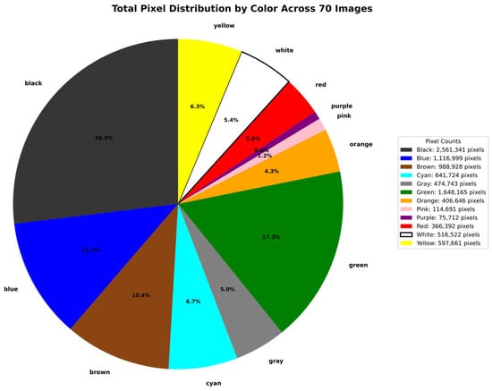
Figure 1. Pie diagram with distribution of 9,509,524 labeled pixels per color in 70 generated images.

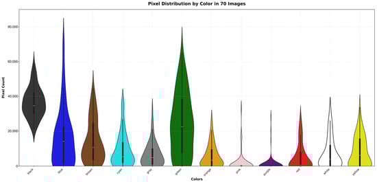
Figure 2. Violin distribution of 9,509,524 labeled pixels per color in 70 generated images.

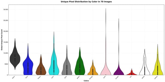
Figure 3. Violin distribution of 1,794,758 unique pixels per color in 70 generated images.

Table 3 presents the descriptive statistics for the color frequency per image in the 70 generated images, including the mean, median, standard deviation (Std), minimum (Min), maximum (Max), quartiles (Q1, Q2, Q3), Interquartile Range (IQR), coefficient of variation (CV), and imbalance ratio (IR), considering black and purple as the maximum and minimum classes, respectively. These metrics enable us to identify the risks associated with an imbalanced dataset and prepare sampling algorithms to address these issues before working with it. Almost all images contain specific colors related to landscaping and stained-glass structures, such as black, green, blue, and brown. In contrast, other colors have a lower frequency, since they are used in ornaments of the stained-glass art. However, even purple, which is the least frequent color, has 75,712 positive labeled pixels and a mean of 1081.6 instances per image. Additionally, we present in Figure 4 the histogram of frequency for each color in the 70 generated images.

Table 3. Descriptive statistics of color frequency in the 70 generated images.

Color	Mean	Median	Std	Min	Max	Q1	Q3	IQR	Total Pixels	CV	IR
Black	36,590.59	34,725.5	8449.07	20,930	58,512	30,492	41,802	11,310	2,561,341	23.09	33.83
Blue	15,957.13	14,136	16,824.37	0	70,719	2111.75	22,314.25	20,202.5	1,116,999	105.43	14.75
Brown	14,127.54	10,651.5	12,105.43	341	44,518	3767	24,556.25	20,789.25	988,928	85.69	13.06
Cyan	9167.49	5296.5	9546.56	0	36,150	2262.75	13,382	11,119.25	641,724	104.13	8.47
Gray	6782.04	4843.5	6968.1	0	32,852	1310.75	9578.5	8267.75	474,743	102.74	6.27
Green	23,545.21	22,543.5	17,632.6	3	64,868	7973.75	38,159.25	30,185.5	1,648,165	74.89	21.77
Orange	5809.23	3325.5	6565.97	0	26,679	476.25	9199.5	8723.25	406,646	113.03	5.37
Pink	1638.44	0	5426.37	0	32,869	0	3.75	3.75	114,691	331.19	1.51
Purple	1081.6	1	4474.08	0	28,136	0	34	34	75,712	413.65	1.00
Red	5234.17	465	7551.47	0	28,212	1	7656.5	7655.5	366,392	144.27	4.84
White	7378.89	3830	8762.1	0	32,099	559.5	11,657.25	11,097.75	516,522	118.75	6.82
Yellow	8538.01	6115.5	8691.35	0	33,670	307.5	15,319.75	15,012.25	597,661	101.8	7.89

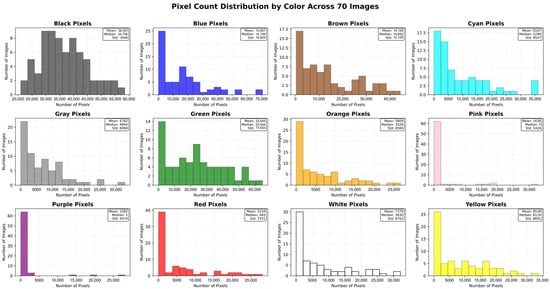
Figure 4. Histogram frequency of 9,509,524 labeled pixels per color in 70 generated images.

Given the imbalanced dataset resulting from the natural color distribution in the generated images, which is inherited from the content of the internet stained-glass images used for training the DALL·E 3 model, we include RGB channel descriptive statistics and distributions per color in Table 4 and Figure 5 to prove that there are sufficient pixels per color to exhibit a rich channel distribution, which is valuable when training machine learning models. The distributions of other color spaces are also available in the dataset.

Table 4. Descriptive statistics of RGB channels per color in the 70 generated images.

Color	Channel	Count	Mean	Median	Std	Min	Max	Q1	Q3	IQR	CV	Range
Black	R	2,561,341	27.41	8	45.46	0	255	1	32	31	165.84	255
Black	G	2,561,341	29	13	38.43	0	255	4	39	35	132.53	255
Black	B	2,561,341	14.66	2	31.12	0	255	0	12	12	212.3	255
Blue	R	1,116,999	8.18	1	18.26	0	255	0	6	6	223.14	255
Blue	G	1,116,999	56.86	55	35.21	0	255	31	79	48	61.92	255
Blue	B	1,116,999	83.43	78	53.04	0	255	44	120	76	63.58	255
Brown	R	988,928	78.66	71	55.08	0	255	35	114	79	70.02	255
Brown	G	988,928	48.31	38	41.87	0	255	15	71	56	86.68	255
Brown	B	988,928	9.04	1	21.09	0	255	0	7	7	233.31	255
Cyan	R	641,724	45.46	34	44.69	0	255	5	73	68	98.31	255
Cyan	G	641,724	100.8	102	51.37	0	255	64	137	73	50.96	255
Cyan	B	641,724	102.35	101	58.31	0	255	58	144	86	56.97	255
Gray	R	474,743	90.09	86	54.39	0	255	51	128	77	60.37	255
Gray	G	474,743	93.03	94	50.12	0	255	63	126	63	53.87	255
Gray	B	474,743	64.27	59	45.77	0	255	30	91	61	71.21	255
Green	R	1,648,165	43.09	37	36.78	0	255	13	64	51	85.36	255
Green	G	1,648,165	65.37	62	40.65	0	255	37	90	53	62.18	255
Green	B	1,648,165	19.35	4	29.66	0	255	0	30	30	153.27	255
Orange	R	406,646	145.31	157	63.75	0	255	109	194	85	43.87	255
Orange	G	406,646	82.19	83	48.21	0	255	44	116	72	58.66	255
Orange	B	406,646	8.23	2	17.93	0	244	0	7	7	217.71	244
Pink	R	114,691	141.72	153	66.48	0	255	102	194	92	46.91	255
Pink	G	114,691	77.93	74	49.53	0	254	39	115	76	63.56	254
Pink	B	114,691	83.09	86	48.76	0	250	47	120	73	58.68	250
Purple	R	75,712	62.68	62	36.89	0	255	36	85	49	58.85	255
Purple	G	75,712	38.75	34	33.12	0	255	9	59	50	85.48	255
Purple	B	75,712	98.87	105	57.16	0	255	54	144	90	57.82	255
Red	R	366,392	121.81	124	66.65	0	255	70	177	107	54.71	255
Red	G	366,392	15.8	9	20.48	0	255	3	21	18	129.61	255
Red	B	366,392	3.27	0	12.81	0	230	0	1	1	392.18	230
White	R	516,522	171.51	185	57.32	0	255	148	212	64	33.42	255
White	G	516,522	156.85	169	55.93	0	255	132	197	65	35.66	255
White	B	516,522	114.55	118	57.64	0	255	76	157	81	50.31	255
Yellow	R	597,661	161.61	177	62.64	0	255	131	208	77	38.76	255
Yellow	G	597,661	128.1	136	54.54	0	255	98	168	70	42.57	255
Yellow	B	597,661	37.98	24	41.19	0	255	4	61	57	108.44	255

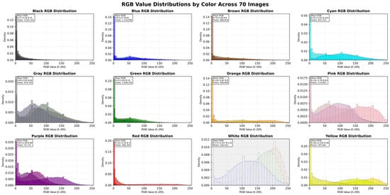
Figure 5. Histogram RGB channel distribution for 9,509,524 labeled pixels per color.

The channel distribution histograms (Figure 5) confirm that each color class in the dataset is characterized by a clear and consistent dominant channel pattern. The red, green, and blue have a single dominant channel (R, G, and B, respectively). Composite colors, such as yellow and orange, have a strong concentration in R and G, with a lower one in B. Similarly, cyan presents high concentrations for G and B, with a lower one in R. These distributions show that the dataset captures the chromatic logic expected for each color category.

Moreover, the histograms highlight the color variability, with distributions spread across a range of values. These distributions, with rich ranges in the channels for each color, provide a high-variability dataset to test machine learning algorithms that learn color boundaries instead of memorizing the values of pixels. For instance, purple shows contributions from R and B, producing an overlap within B; pink strongly depends on R but also has larger values of G and B, resulting in lighter tones.

We also include a 3D representation of the colors in VitralColor-12 in RGB space (Figure 6), HSL space (Figure 7), and CIELAB space (Figure 8). To achieve this, we randomly sample 20,000 points per color, resulting in a total of 240,000 points, and then plot each point with its corresponding color. This shows the variability of colors in the proposed dataset.

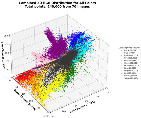
Figure 6. Three-dimensional plot of RGB space with randomly sampled 240,000 points.

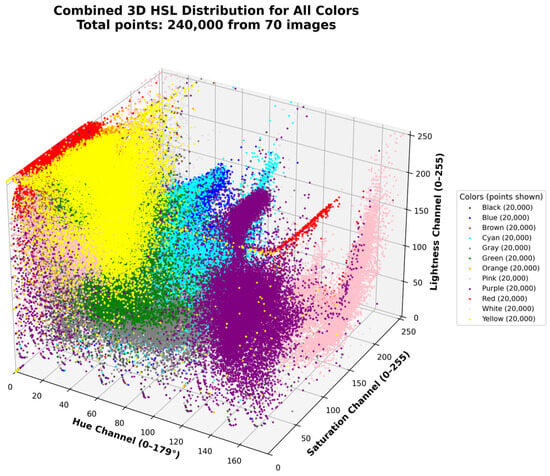
Figure 7. Three-dimensional plot of HSL space with randomly sampled 240,000 points.

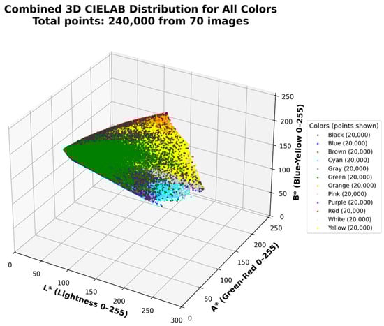
Figure 8. Three-dimensional plot of CIELAB space with randomly sampled 240,000 points per color.

We also include the chromaticity diagram across channels a and b in the CIELAB representation (Figure 9) to visually compare the distance between colors and the difference in frequency due to the natural imbalanced distribution of colors in stained-glass images. Moreover, we also obtain the ΔE76 and ΔE94 standardized dissimilarity metrics using the CIELAB 1976 and 1994 conventions, as shown in Figure 10.

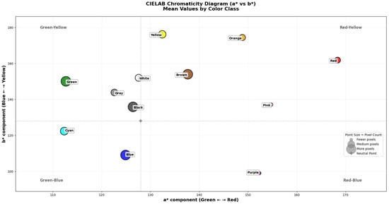
Figure 9. Chromacity a vs. b in CIELAB space with 9,509,524 labeled pixels per color.

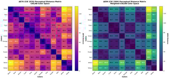
Figure 10. ΔE76 and ΔE94 CIELAB dissimilarity perception for 9,509,524 labeled pixels per color in 70 generated images.

The results in ΔE76 and ΔE94 reveal several important characteristics. First, the dataset is organized into clear perceptual families: warm colors such as red, orange, yellow, and brown form a compact group, with distances dropping from 46.4 ΔE76 to 40.5 ΔE94 (red to orange) and from 25.7 ΔE76 to 6.6 ΔE94 (green to brown), showing that these classes occupy near regions in the space. Similarly, the cold tones blue, purple, cyan, and green are closer to each other compared with warm colors. The neutral classes (black, gray, white) maintain large separations from saturated colors.

Black and white remain as the most distant colors (135.7 ΔE76 and 134.8 ΔE94), with a greater perceptual contrast. Yellow and white decrease in distance from 34.5 ΔE76 to 24.5 ΔE94, showing that they remain related but still distinct. On the other hand, purple and white, like blue and white, maintain very large distances (>100).

These observations demonstrate that the dataset not only covers a balanced variety of hues but also captures how perceptual similarity and contrast naturally distribute among classes.

3. Methods

VitralColor-12 basis images are generated using DALL·E 3 within the ChatGPT platform (https://chatgpt.com/), utilizing the GPT-5 model. Therefore, they are free of copyright restrictions for use. By generating the basis images for labeling using an LLM, we can query any style of images. We decided to work with stained-glass images. The steel structure that supports the colored glass serves as a segmentation guide, with borders that define the colors. This simplifies the segmentation process.

To save processing time and use of computational resources, we generate twelve images together, arranged in a grid. We use a size of 1024 × 1536 pixels, which matches what DALL·E-3 allows. After generation, we split the grid into separate images for labeling.

We manually labeled each stained-glass image by selecting centroid points for each color. These are recorded in a CSV file. We marked at least one central point—with Hue, Saturation, and Lightness (HSL) color values—within each region defined by steel structures. This limits the pixels that need labeling. We then obtain clusters per color based on these centroid points.

After finding color groups, we assign each pixel in the image to a color and make a mask for each color. Then we save the unique pixels for every color in separate CSV files.

The complete process for generating the partially synthetic VitralColor-12 dataset is shown in Figure 11.

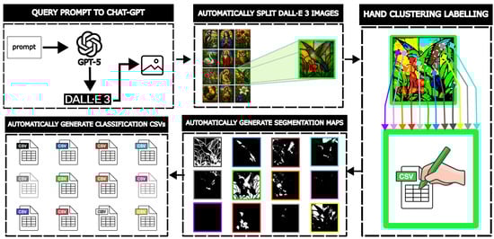
Figure 11. Process for generating the partially synthetic VitralColor-12 with GPT-5 and DALL·E-3 models.

3.1. Query Prompt to Chat-GPT

The prompt used was adapted and tested several times to achieve our requirements, which take into consideration several elements:

• First, select the image size of 1024 × 1536 pixels, as the DALL·E-3 model only supports specific resolutions [39].
• Define that the generated images must be stained-glass photos.
• Define the resolution of each stained-glass image as 322 × 390 pixels. This ensures similar sizes for all images and simplifies the splitting process. We chose this size to fit the grid of images.
• Indicate the grid structure using the selected sizes for the stained-glass images and total image size. Use a 4-column by 3-row grid, which fits the selected resolutions.
• Indicate having white frames between each stained-glass image to simplify the splitting process.
• Indicate the color of the structure supporting the glass. This makes it easy to identify the different color regions during labeling.

Additionally, we include extra information to avoid incomplete images and maintain the desired structure, which were the elements that the model had difficulties with.

After several tests and help to improve it from the GPT-5 model, the prompt achieved all the requirements. The textual prompt is as follows:

“Create a single image sized 1024 × 1536 pixels. It must contain exactly 12 separate stained-glass photographs, each exactly rectangular and the same size (322 × 390 pixels). Arrange them in a precise 4-column by 3-row grid. Between each photo, include clear white frames (color 255,255,255), with visible white borders at the top and bottom edges of the image. Each stained-glass photo should have a dark supporting frame and must not be cropped or cut off. All 12 should be complete, equal in width and height, and aligned perfectly in the grid. The photos should be unique, showing stained glass designs of flowers, animals, and religious scenes, with realistic illumination and visible background light effects.”

Figure 12 shows three images obtained with the prompt. It produces photos of stained-glass pictures, featuring a variety of colors and dark structures supporting the glass, white frames dividing each image, and a 4-column by 3-row grid. However, the sizes of images are not maintained consistently. Moreover, at present, it is not possible to control the random seed in the Chat-GPT platform with the DALL·E-3 model; thus, the results may differ even when using the same prompt.

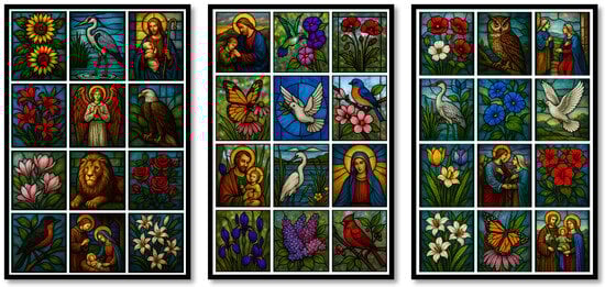
Figure 12. Examples of grids of stained-glass images generated with the same prompt.

3.2. Automatically Split Dall·E 3 Images

Since the generated images vary in size, the splitting algorithm must determine the coordinates for cropping them. The algorithm begins with the generated image $I_{color}$, which contains the 12 stained-glass images. The $I_{color}$ comprises three matrices, one for each color channel, $R^{i\times j}$, $G^{i\times j}$, and $B^{i\times j}$, with $i=\mathrm{1,2},3\dots ,rows$ and $j=\mathrm{1,2},3,\dots ,cols$. Since we use the white frames to divide the image, we do not need information about the colors at this stage; thus, we use Equation (1) to convert the color matrices into a single matrix, $I_{gray}$, representing the image in grayscale converted with the luminosity method [40].

$$I_{gray}=0.3\times R+0.59\times G+0.11\times B$$

(1)

After that, we determine$iw$ and $jw$, all the rows and columns associated with white pixels in the image, detected by thresholding $I_{gray}$ with $th=128$, as in Equations (2) and (3).

$$iw=\{i\left|I_{gray}\left(i,j\right)>th\right\}$$

(2)

$$jw=\{j\left|I_{gray}\left(i,j\right)>th\right\}$$

(3)

Then, we take $iw$ and $jw$, containing $a$ and $b$ elements, respectively, to create groups maintaining a distance tolerance of $\delta$ around the same group, if not adding another one. Those groups, $g{i}_m$ and $g{j}_n$, allow us to obtain $m$ and $n$ groups of coordinates pointing to the same frame side, as in Equations (4) and (5).

$${gi}_m=\{iw\left(a\right)\left|\left|iw\left(a\right)-iw\left(a-1\right)\right|\le \delta \right\}$$

(4)

$$g{j}_n=\left\{jw\left(b\right)\right|\left|jw\left(b\right)-jw\left(b-1\right)\right|\le \delta \}$$

(5)

Once we group the near-white pixels with a $\delta$ tolerance, we can determine the $x_o$ and $y_p$ coordinates for cropping stained-glass images with Equations (6) and (7), where $o$ and $p$ denote the number of cuts to perform, and the operator $\lfloor \rfloor$ indicates the floor.

$$x_o=\lfloor \frac{1}{m}\sum _{k = 1}^{m}g{i}_k\rfloor$$

(6)

$$y_p=\lfloor \frac{1}{n}\sum _{k = 1}^{n}g{j}_k\rfloor$$

(7)

Finally, we obtain each stained-glass image by cropping the coordinates of the original color image and saving the result image.

3.3. Hand Clustering Labeling

The labeling process begins by presenting a generated stained-glass image, after which the user must select at least one central point pixel for each color in the regions marked, with the stained-glass structures in dark colors. When a color is not in the image, the user must provide a central point with a centroid corresponding to that color captured from another image. The centroid points are obtained in the HSL space and registered in a CSV file. We obtain the HSL values by using the color picker tool from Microsoft PowerToys 0.94. Figure 13 shows the labeling system capturing a centroid point for the white color.

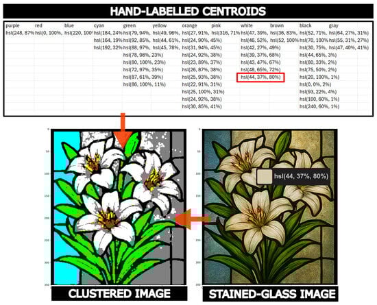
Figure 13. Labeling system in VitralColor-12, obtaining a centroid point with the color picker tool from PowerToys.

Once at least a centroid per color is captured, we calculate $D_c$, the Euclidean distance between each pixel $P\left(p_H,p_S,p_L\right)$ to the centroids for each color $C\left(c_H,c_S,c_L\right)$ with Equation (8). Then, we assign the $P$ to the color $C$ with the minimum color distance. The system displays the results, showing the image again with the changed pixel colors corresponding to the label. Additionally, we perform two iterations of the dilation and erosion process to close open points using a kernel of 2 pixels. This process reduces noise in the image, but it discards smaller regions.

$$D_c=\sqrt{{\left(p_H-c_H\right)}^2+{\left(p_S-c_S\right)}^2+{\left(p_L-c_L\right)}^2}$$

(8)

3.4. Automatically Generate Segmentation Maps

We build segmentation maps in 12 black images, one for each color, with all their pixels being $\left(\mathrm{0,0},0\right)$ and the same size of the original image; then, we change the pixels to white $\left(\mathrm{255,255,255}\right)$ for a corresponding mask in the same pixel location if they belong to the color, based on the centroid and $D_c$ in Equation (8), as shown in Figure 14.

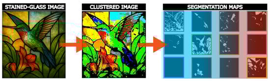
Figure 14. Segmentation maps and labeling results with VitralColor-12.

3.5. Automatically Generate Classification CSVs

Finally, we use the R, G, B values in the corresponding pixel location to identify if the pixel belongs to the color, based on the centroid and $D_c$ in Equation (8). Then, we use the cvtColor method of OpenCV to convert from the RGB color space to obtain HSL, CIELAB, and YCbCr values, allowing users to classify colors in any of these representations or use them to create new segmentation maps, following the approach in Section 3.4.

Table 5 presents an example of a single pixel with the available data in the VitralColor-12 CSV files. It includes the pixel’s corresponding color, the image row and column where the pixel was found, the RGB, HSL, CIELAB, and YCbCr values, and mean lightness determined with 4 and 8 neighborhoods.

Table 5. VitralColor-12 classification data available in CSV files for a pixel belonging to the green color.

Color	Image_Index	Row	Col	RGB_R	RGB_G	RGB_B	HSL_H	HSL_S	HSL_L	CIELAB_L	CIELAB_A	CIELAB_B	YCbCr_Y	YCbCr_Cb	YCbCr_Cr	Lightness 4	Lightness 8
Green	1	9	11	1	64	50	83	247	32	60	105	132	44	97	131	32.25	32.375

4. User Notes

The VitralColor-12 dataset is a naturally imbalanced dataset due to the inherent nature of working with generated images inspired by stained glass (we included an imbalance ration in the descriptive statistics for the pixel frequency across images in Table 3). These images produce more pixels with green, blue, black, and gray, which are the most frequently used colors in landscaping (trees, grass, sky, water) and steel structures. The less common colors are white, purple, pink, cyan, orange, and red, as they are not popular in stained glass or are used only ornamentally.

Users should note that the DALL·E model for image generation may introduce biases in cultural and lighting conditions, which are inherited from internet content about stained-glass images. These biases can influence the dataset’s representativeness and fairness when applied in various applications. Thus, we recommend that users evaluate these aspects closely and consider such biases when deploying the dataset by incorporating validation sets or cross-domain tests to measure the effects of such biases. A robust evaluation strategy, including cross-domain tests, can provide reassurance by demonstrating how VitralColor-12 performs across different contexts. To improve the dataset’s balance for training machine learning models, we recommend using techniques such as undersampling, oversampling, smoothing, or other data balancing algorithms. Alternatively, we recommend training a model for each color separately.

VitralColor-12 was produced with hand notations for the centroids per color. Since these notations were created by hand, they are likely to contain notation errors with a certain probability. We did not exclude those errors or outlier colors; therefore, we recommend using the Z-score, IQR (which we included in the descriptive statistics for the RGB channel in Table 4), Mahalanobis Distance, Variance Threshold, or another technique to remove outliers.

Pixels belonging to a color that is not one of the 12 available colors are labeled as one of them. Future work on the dataset will include more colors, but in this version the user must take this into consideration. For example, colors like skin, maroon, khaki, magenta, turquoise, or olive are mislabeled as brown, orange, yellow, pink, blue, or green.

The segmentation maps in this version were generated using the centroid points for clustering pixels based on Euclidean distance, but this method is sensitive to noise. However, the centroid points can be used in conjunction with other algorithms to generate more effective segmentation masks, such as edge detection, histograms, artificial intelligence techniques, or other methods. Future work on VitralColor-12 includes adding more segmentation maps using different algorithms.

5. Conclusions

In this work, we developed VitralColor-12, a synthetic dataset for color classification and segmentation that uses LLMs, specifically GPT-5 and DALL·E 3, to generate images of stained glass that simplify color segmentation by using as a guide the dark steel structure supporting the glass.

Unlike the existing datasets, which are limited by domain, color range, or annotation tools, our proposal offers 12 color classes in 70 images, each accompanied by segmentation maps. For classification, it includes 9,509,524 labeled pixels, of which 1,794,758 are unique. VitralColor-12’s extensive data make it an alternative for benchmarking algorithms or applications with different purposes related to color classification or segmentation.

Moreover, we supply violin diagrams with the frequency of colors across images, histograms of channels per color, 3D color maps, and descriptive statistics. Additionally, we provide standardized metrics, such as ΔE76, ΔE94, and Chromacity a vs. b in the CIELAB space, which show the rich distribution of the labeled colors and their applicability, proving that our dataset accurately reproduces realistic perceptual structures, including warm, neutral, and cold colors, as well as the contrast between black and white. Furthermore, this validates that the dataset produces meaningful perceptual clusters, reinforcing its utility for color segmentation and classification.

The channel distribution histograms confirm that each color exhibits a distinct dominant channel, with variability in its mean and standard deviation, as well as overlaps in perceptually consistent regions. This ensures that the dataset is sufficiently diverse and representative for training machine learning models.

VitralColor-12 provides a standardized alternative dataset for color segmentation, featuring characteristics that address gaps in the publicly available resources, offering detailed color descriptions, variation analysis, channel distributions, and standardized metrics.

Future Work

VitralColor-12 could include additional colors by following the same approach in this work; therefore, future versions will add extra colors, such as skin, maroon, khaki, magenta, turquoise, or olive tones. Moreover, later versions could include other algorithms to generate segmentation maps, such as edge detection, histograms, and artificial intelligence techniques, instead of only working with Euclidean distance.

References

- Cheng, H.D.; Jiang, X.H.; Sun, Y.; Wang, J. Color Image Segmentation: Advances and Prospects. Pattern Recognit. 2001, 34, 2259–2281. [Google Scholar] [CrossRef]
- Al Garea, S.; Das, S. Image Segmentation Methods: Overview, Challenges, and Future Directions. In Proceedings of the 2024 7th International Women in Data Science Conference at Prince Sultan University, WiDS-PSU 2024, Riyadh, Saudi Arabia, 3–4 March 2024; pp. 56–61. [Google Scholar] [CrossRef]
- Yu, Y.; Wang, C.; Fu, Q.; Kou, R.; Huang, F.; Yang, B.; Yang, T.; Gao, M. Techniques and Challenges of Image Segmentation: A Review. Electronics 2023, 12, 1199. [Google Scholar] [CrossRef]
- Lei, T.; Jia, X.; Zhang, Y.; Member, S.; Liu, S.; Meng, H.; Nandi, A.K.; Nandi, A.K. Superpixel-Based Fast Fuzzy C-Means Clustering for Color Image Segmentation. IEEE Trans. Fuzzy Syst. 2019, 27, 1753–1766. [Google Scholar] [CrossRef]
- Ansari, M.A.; Singh, D.K. Significance of Color Spaces and Their Selection for Image Processing: A Survey. Recent Adv. Comput. Sci. Commun. 2021, 15, 946–956. [Google Scholar] [CrossRef]
- Khaung, A.M.; Stiffler, N.M.; Stiffler, N.M. Intelligent Motion Tracking: A Low-Cost Surveillance Framework Using SoC Devices and Sensor Fusion. Proc. Berry Summer Thesis Inst. 2025, 4, 35–47. [Google Scholar]
- Zhu, S.; Liu, Z.; Letchmunan, S.; Qiu, H. Auto Feature Weighted C-Means Type Clustering Methods for Color Image Segmentation. Eng. Appl. Artif. Intell. 2025, 153, 110768. [Google Scholar] [CrossRef]
- Sodjinou, S.G.; Mohammadi, V.; Sanda Mahama, A.T.; Gouton, P. A Deep Semantic Segmentation-Based Algorithm to Segment Crops and Weeds in Agronomic Color Images. Inf. Process. Agric. 2022, 9, 355–364. [Google Scholar] [CrossRef]
- Hasan, S.; Jahan, S.; Islam, M.I. Disease Detection of Apple Leaf with Combination of Color Segmentation and Modified DWT. J. King Saud Univ.-Comput. Inf. Sci. 2022, 34, 7212–7224. [Google Scholar] [CrossRef]
- Liu, W.; Sun, H.; Xia, Y.; Kang, J. Real-Time Cucumber Target Recognition in Greenhouse Environments Using Color Segmentation and Shape Matching. Appl. Sci. 2024, 14, 1884. [Google Scholar] [CrossRef]
- Waldamichael, F.G.; Debelee, T.G.; Ayano, Y.M. Coffee Disease Detection Using a Robust HSV Color-Based Segmentation and Transfer Learning for Use on Smartphones. Int. J. Intell. Syst. 2022, 37, 4967–4993. [Google Scholar] [CrossRef]
- Kusumandari, D.E.; Adzkia, M.; Gultom, S.P.; Turnip, M.; Turnip, A. Detection of Strawberry Plant Disease Based on Leaf Spot Using Color Segmentation. J. Phys. Conf. Ser. 2019, 1230, 012092. [Google Scholar] [CrossRef]
- Song, H.; Wang, J.; Bei, J.; Wang, M. Modified Snake Optimizer Based Multi-Level Thresholding for Color Image Segmentation of Agricultural Diseases. Expert Syst. Appl. 2024, 255, 124624. [Google Scholar] [CrossRef]
- Ganesan, P.; Sathish, B.S.; Leo Joseph, L.M.I.; Sajiv, G.; Murugesan, R.; Akilandeswari, A.; Gomathi, S. HSV Model Based Skin Color Segmentation Using Uncomplicated Threshold and Logical AND Operation. In Proceedings of the 2023 9th International Conference on Advanced Computing and Communication Systems, ICACCS 2023, Coimbatore, India, 17–18 March 2023; pp. 415–419. [Google Scholar] [CrossRef]
- Benčević, M.; Habijan, M.; Galić, I.; Babin, D.; Pižurica, A. Understanding Skin Color Bias in Deep Learning-Based Skin Lesion Segmentation. Comput. Methods Programs Biomed. 2024, 245, 108044. [Google Scholar] [CrossRef]
- Staal, J.; Abràmoff, M.D.; Niemeijer, M.; Viergever, M.A.; Van Ginneken, B. Ridge-Based Vessel Segmentation in Color Images of the Retina. IEEE Trans. Med. Imaging 2004, 23, 501–509. [Google Scholar] [CrossRef] [PubMed]
- Tang, S.; Yu, F. Construction and Verification of Retinal Vessel Segmentation Algorithm for Color Fundus Image under BP Neural Network Model. J. Supercomput. 2021, 77, 3870–3884. [Google Scholar] [CrossRef]
- Xia, P.; Wang, S.; Gong, F.; Cao, W.; Zhao, Y. Rapid Recognition Method of Red Brick Content in Recycled Brick-Concrete Aggregates and Powder Based on Color Segmentation. J. Build. Eng. 2024, 84, 108633. [Google Scholar] [CrossRef]
- Van Do, Q.; Hoang, H.T.; Van Vu, N.; De Jesus, D.A.; Brea, L.S.; Nguyen, H.X.; Nguyen, A.T.L.; Le, T.N.; Dinh, D.T.M.; Nguyen, M.T.B.; et al. Segmentation of Hard Exudate Lesions in Color Fundus Image Using Two-Stage CNN-Based Methods. Expert Syst. Appl. 2024, 241, 122742. [Google Scholar] [CrossRef]
- Barnard, K.; Martin, L.; Funt, B.; Coath, A. A Dataset for Color Research. Color Res. Appl. 2002, 27, 147–151. [Google Scholar] [CrossRef]
- Laura, F. Computer Vision with Seedlings. Available online: https://www.kaggle.com/code/allunia/computer-vision-with-seedlings (accessed on 1 September 2025).
- Dev, S.; Lee, Y.H.; Winkler, S. Color-Based Segmentation of Sky/Cloud Images from Ground-Based Cameras. IEEE J. Sel. Top. Appl. Earth Obs. Remote Sens. 2017, 10, 231–242. [Google Scholar] [CrossRef]
- Bhatt, R.B.; Dhall, A.; Sharma, G.; Chaudhury, S. Efficient Skin Region Segmentation Using Low Complexity Fuzzy Decision Tree Model. In Proceedings of the INDICON 2009—An IEEE India Council Conference, Ahmedabad, India, 18–20 December 2009. [Google Scholar] [CrossRef]
- Rajen, B. Abhinav Dhall Skin Segmentation—UCI Machine Learning Repository. Available online: https://archive.ics.uci.edu/dataset/229/skin+segmentation (accessed on 1 September 2025).
- ICT Institute Legocolor Dataset. Available online: https://www.kaggle.com/datasets/ictinstitute/legocolor-dataset/code (accessed on 1 September 2025).
- Edge Impulse Object Detection—Dice Colors. Available online: https://studio.edgeimpulse.com/public/497418/latest (accessed on 2 September 2025).
- Fasih Color Detection Dataset. Available online: https://universe.roboflow.com/fasih-zjokb/color-detection-mjyhq (accessed on 1 September 2025).
- Martin, D.; Fowlkes, C.; Tal, D.; Malik, J. A Database of Human Segmented Natural Images and Its Application to Evaluating Segmentation Algorithms and Measuring Ecological Statistics. Proc. IEEE Int. Conf. Comput. Vis. 2001, 2, 416–423. [Google Scholar] [CrossRef]
- Lin, T.Y.; Maire, M.; Belongie, S.; Hays, J.; Perona, P.; Ramanan, D.; Dollár, P.; Zitnick, C.L. Microsoft COCO: Common Objects in Context. In Proceedings of the Computer Vision—ECCV 2014, Zurich, Switzerland, 6–12 September 2014; Lecture Notes in Computer Science (including subseries Lecture Notes in Artificial Intelligence and Lecture Notes in Bioinformatics); Springer: Cham, Switzerland, 2014; Volume 8693 LNCS, pp. 740–755. [Google Scholar] [CrossRef]
- Song, Z.; He, Z.; Li, X.; Ma, Q.; Ming, R.; Mao, Z.; Pei, H.; Peng, L.; Hu, J.; Yao, D.; et al. Synthetic Datasets for Autonomous Driving: A Survey. IEEE Trans. Intell. Veh. 2024, 9, 1847–1864. [Google Scholar] [CrossRef]
- Umer, F.; Adnan, N. Generative Artificial Intelligence: Synthetic Datasets in Dentistry. BDJ Open 2024, 10, 1–5. [Google Scholar] [CrossRef] [PubMed]
- Goyal, M.; Mahmoud, Q.H. A Systematic Review of Synthetic Data Generation Techniques Using Generative AI. Electronics 2024, 13, 3509. [Google Scholar] [CrossRef]
- Balyan, R.; Thompson, K.; Iacobelli, F. LLMs for Question-Answer and Synthetic Data Generation and Evaluation. In Generative Systems and Intelligent Tutoring Systems; Springer: Cham, Switzerland, 2026; pp. 17–31. [Google Scholar] [CrossRef]
- Sapkota, R.; Karkee, M. Generative AI in Agriculture: Creating Image Datasets Using DALL.E’s Advanced Large Language Model Capabilities. arXiv 2023, arXiv:2307.08789. [Google Scholar] [CrossRef]
- Ferdousi, R.; Hossain, M.A.; Saddik, A.E. TextureMeDefect: LLM-Based Defect Texture Generation for Railway Components on Mobile Devices. arXiv 2024, arXiv:2410.18085. [Google Scholar] [CrossRef]
- Arora, A.; Arora, A. Generative Adversarial Networks and Synthetic Patient Data: Current Challenges and Future Perspectives. Future Healthc. J. 2022, 9, 190–193. [Google Scholar] [CrossRef]
- Selvaraj, A.; Rethinavalli, S.; Jeyalakshmi, A. An Application of Generative AI: Hybrid GAN-SMOTE Approach for Synthetic Data Generation And Classifier Evaluation on Breast Cancer Dataset. Indian J. Nat. Sci. 2024, 15, 72395–72400. [Google Scholar]
- Selvam, A. Generative Adversarial Networks for Synthetic Data Creation in Manufacturing Process Simulations. J. Artif. Intell. Res. Appl. 2021, 1, 716–757. [Google Scholar]
- OpenAI. What’s New with DALL·E 3? Available online: https://cookbook.openai.com/articles/what_is_new_with_dalle_3?utm_source (accessed on 3 September 2025).
- Bovik, A. Handbook of Image and Video Processing; Elsevier Academic Press: Amsterdam, The Netherlands, 2005; ISBN 9780121197926. [Google Scholar]
Disclaimer/Publisher’s Note: The statements, opinions and data contained in all publications are solely those of the individual author(s) and contributor(s) and not of MDPI and/or the editor(s). MDPI and/or the editor(s) disclaim responsibility for any injury to people or property resulting from any ideas, methods, instructions or products referred to in the content. |
© 2025 by the authors. Licensee MDPI, Basel, Switzerland. This article is an open access article distributed under the terms and conditions of the Creative Commons Attribution (CC BY) license (https://creativecommons.org/licenses/by/4.0/).