
Enhanced and Interpretable Prediction of Multiple Cancer Types Using a Stacking Ensemble Approach with SHAP Analysis


Abstract
1. Introduction
- The design and implementation of a comprehensive ensemble learning framework for multi-cancer prediction, including 12 base models.
- The rigorous evaluation of the models using various performance metrics, including accuracy, recall, precision, F1-score, AUC, Kappa, and MCC statistics.
- Based on the performances of the base models, two stacking-based metamodels are designed and extensively evaluated.
- The transparent assessment of feature importance and the impact of hyperparameters using explainable AI techniques, such as SHAP and feature importance analysis.
2. Related Work
3. Research Methodology
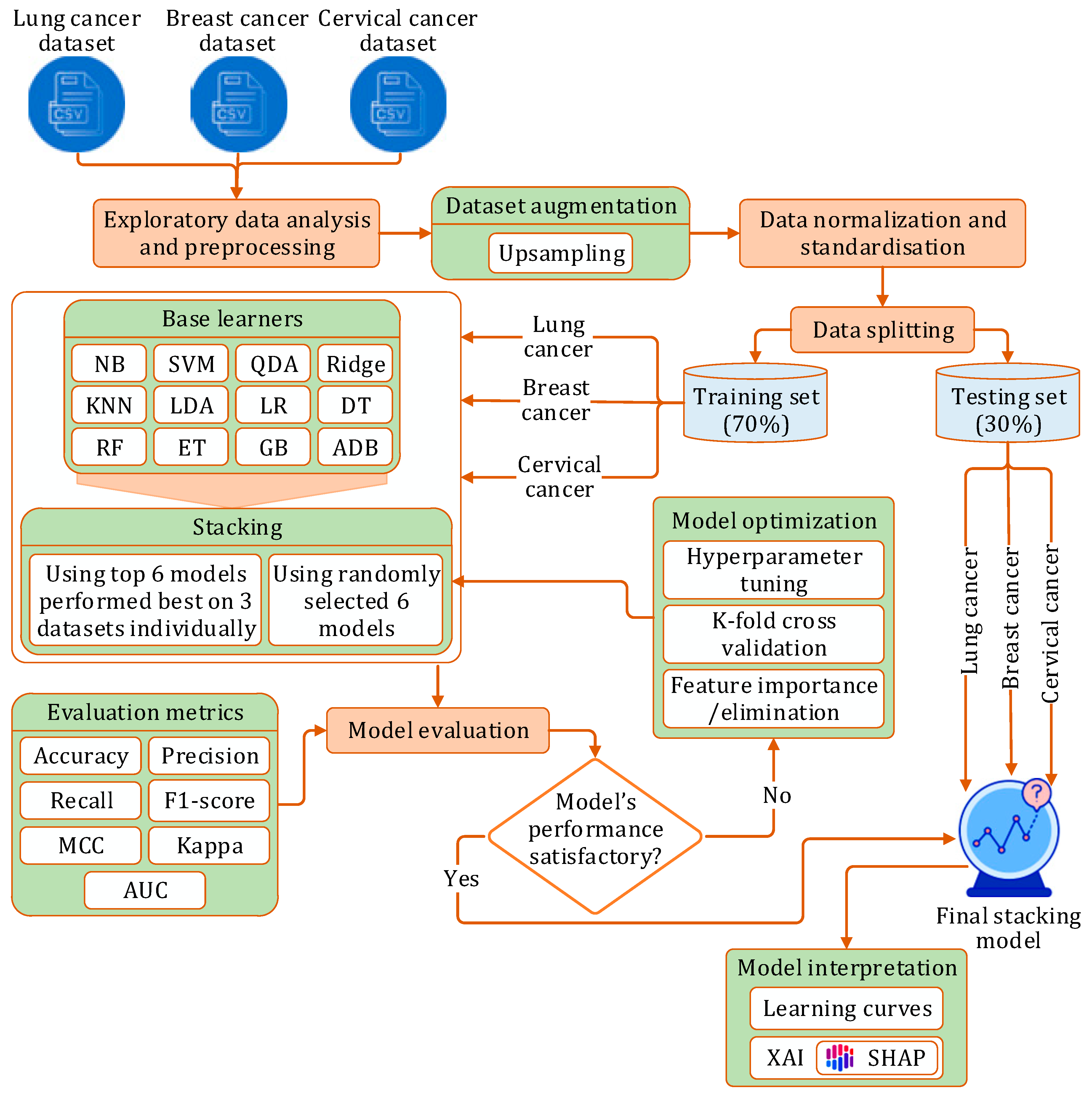
3.1. Research Workflow
- Phase I: We initially implemented twelve prediction models using different machine learning algorithms: NB [41], SVM [42], QDA [43], Ridge [44], KNN [45], LDA [46], LR [47], DT [48], GB [49], ADB [50], RF [51], ET [52]. Each model was implemented on each of the three datasets, with optimization performed through hyperparameter tuning and stratified k-fold cross-validation.
- Phase II: In this phase, we developed a stacking model:
- (a)
- Initially, six randomly picked learners were used to construct the stacking model.
- (b)
- Next, the top six models, which had demonstrated the best performance on each dataset, were selected as constituent learners for the stacking model.
In both scenarios, the model was independently evaluated on each dataset using a comprehensive set of performance metrics, followed by optimization via hyperparameter tuning and stratified k-fold cross-validation.
- Phase III: Finally, we applied XAI techniques to interpret the outcomes of the proposed stacking model.
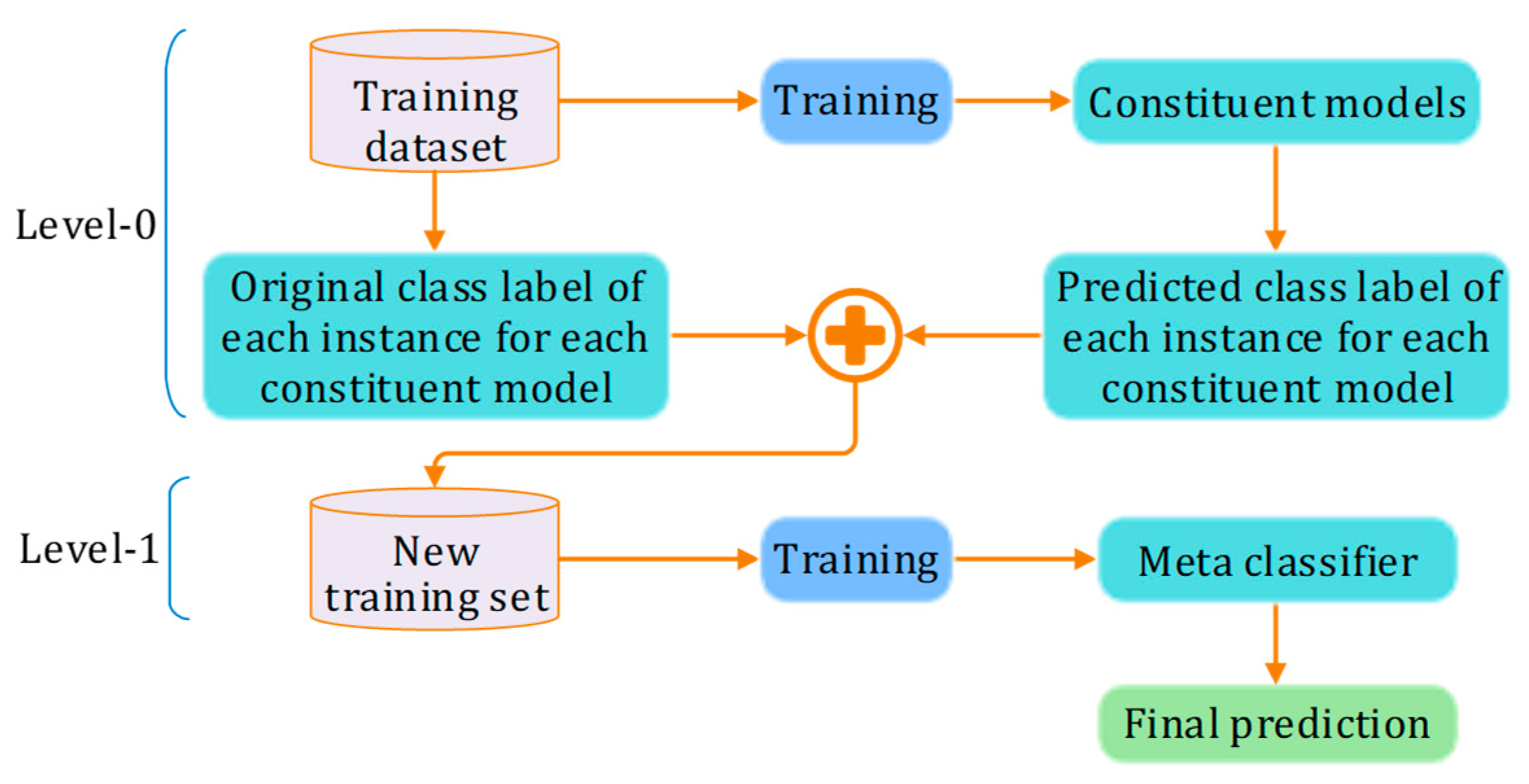
3.2. Stacking
3.3. Experiment Setup
3.4. Evaluation Metrics
4. Dataset Description and Preprocessing
5. Prediction Models and Results
5.1. Base Learner Models
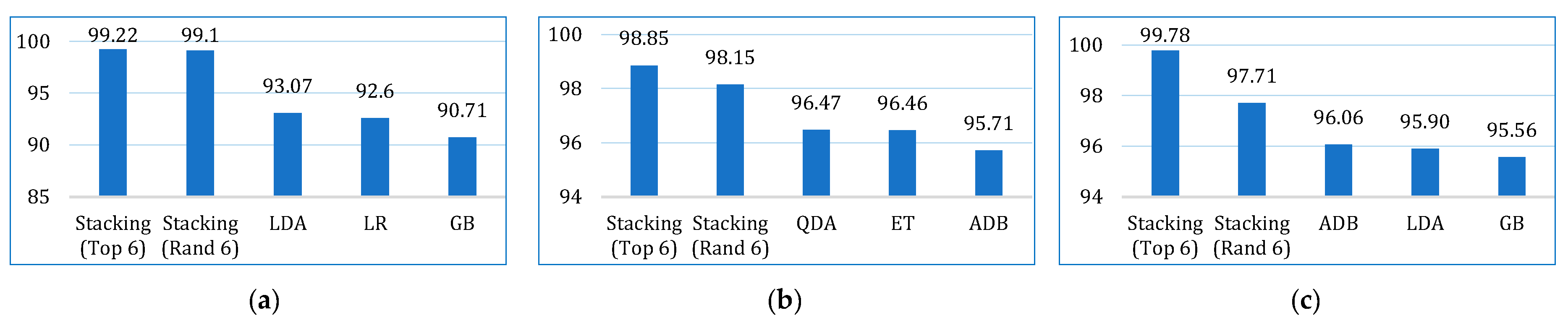
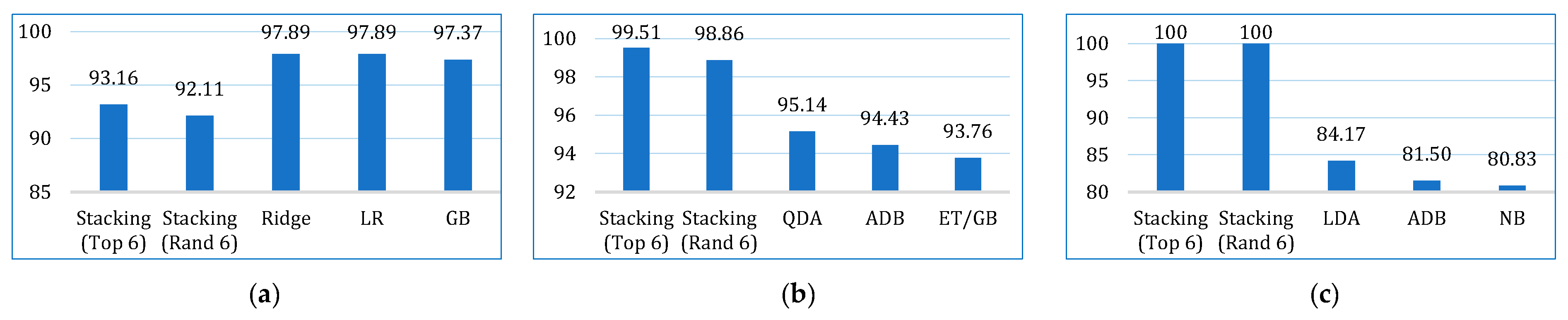
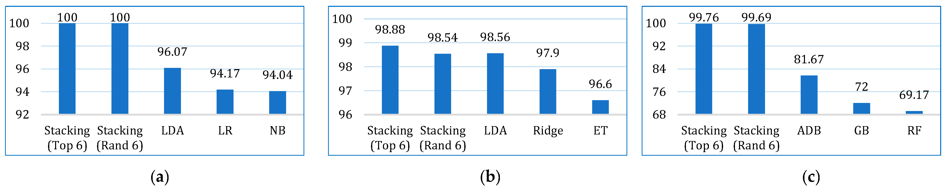
5.2. Stacking Models
- In the first approach, six algorithms (SVM, KNN, DT, ET, GB, ADB) among the twelve were randomly considered. To ensure a comprehensive and robust analysis, we employed three categories of models: base models, Bagging, and Boosting on all three datasets. We selected two models from each category using the ‘random()’ function. Through careful experimentation with various permutations and combinations by executing the `random()` function repetitively, we identified the optimal combination: SVM, KNN, DT, ET, GB, and ADB.
- In the second, the six top-performing algorithms (based on their accuracy) were considered to build the stack. Table 7 shows the top six algorithms for each dataset, as studied in Section 5.1.
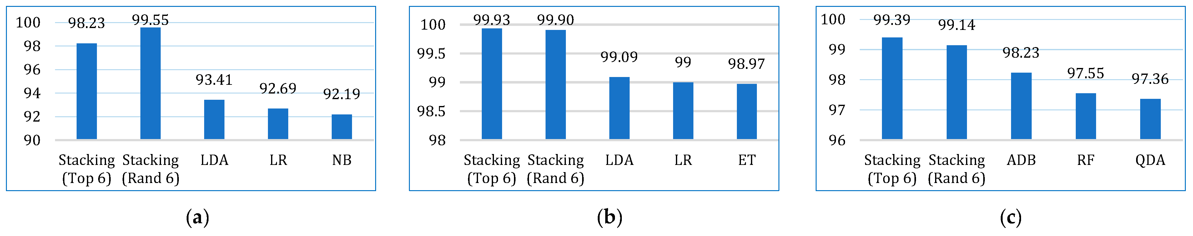
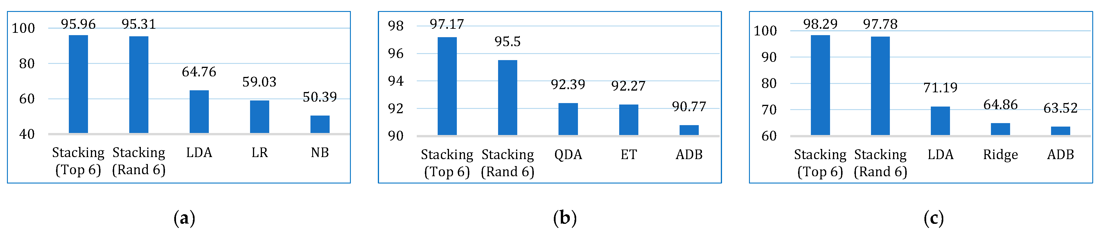
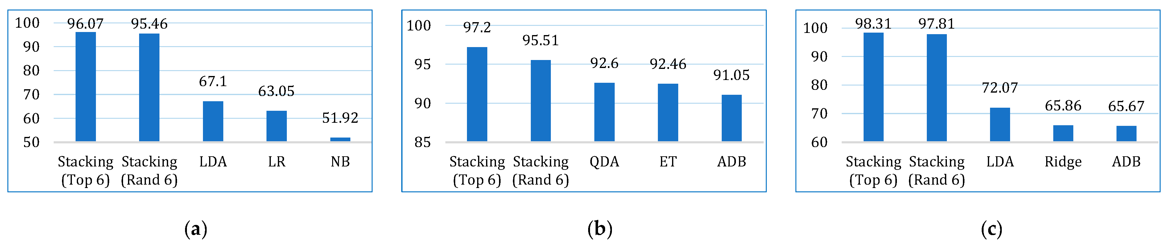
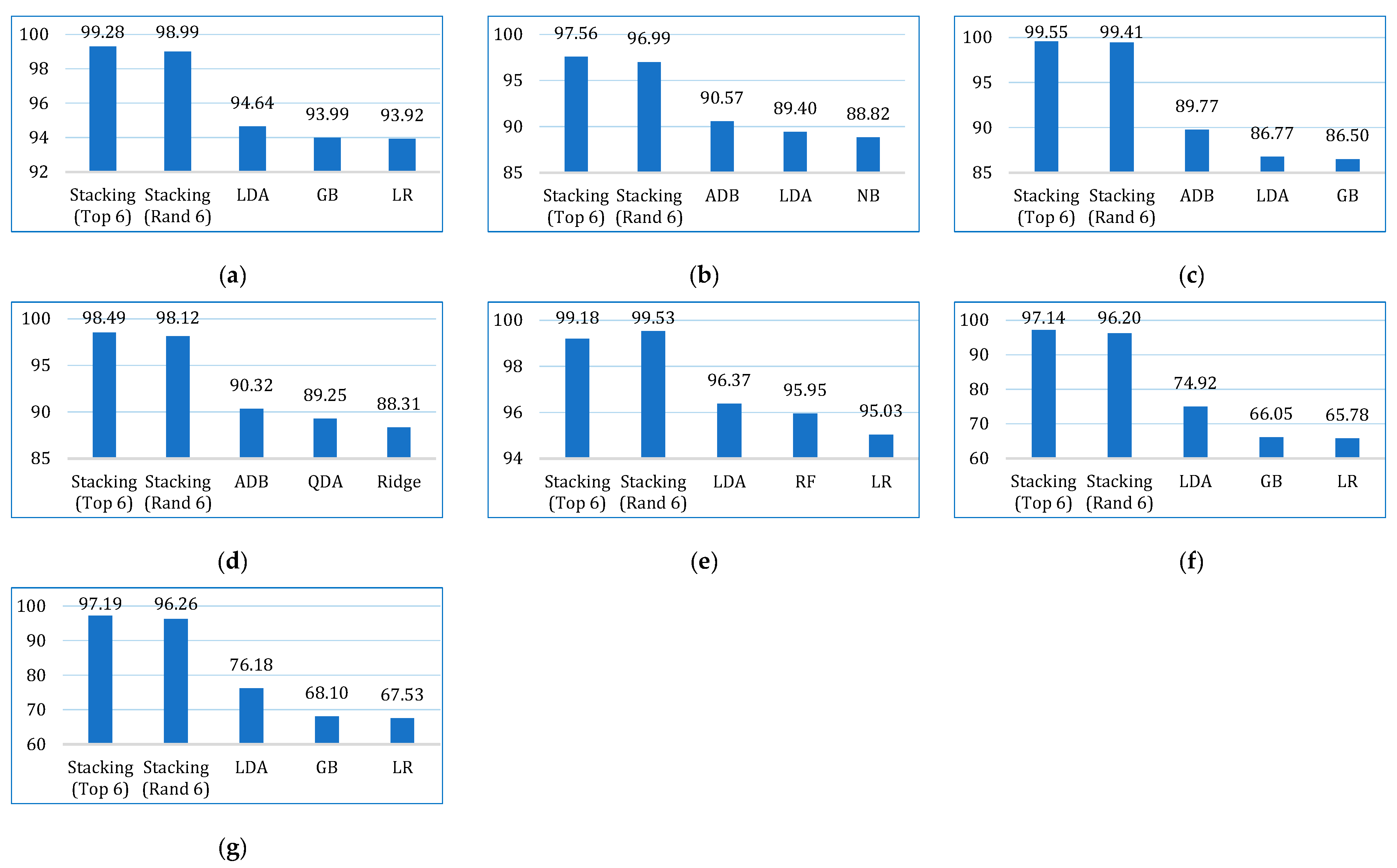
5.3. Comparative Analysis
5.3.1. Comparing with Other Models
5.3.2. Comparing with State-of-the-Art
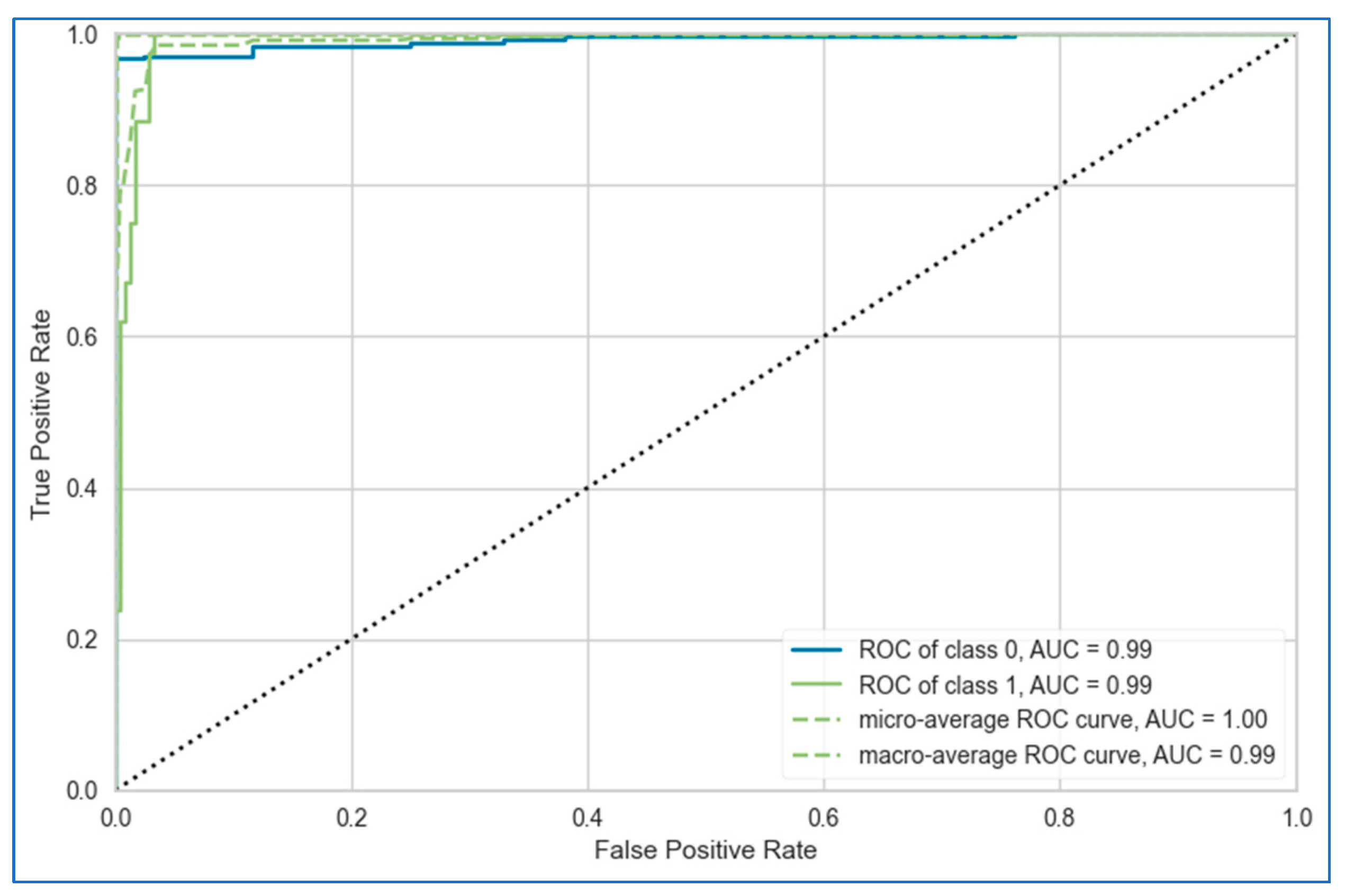
6. Model Interpretation
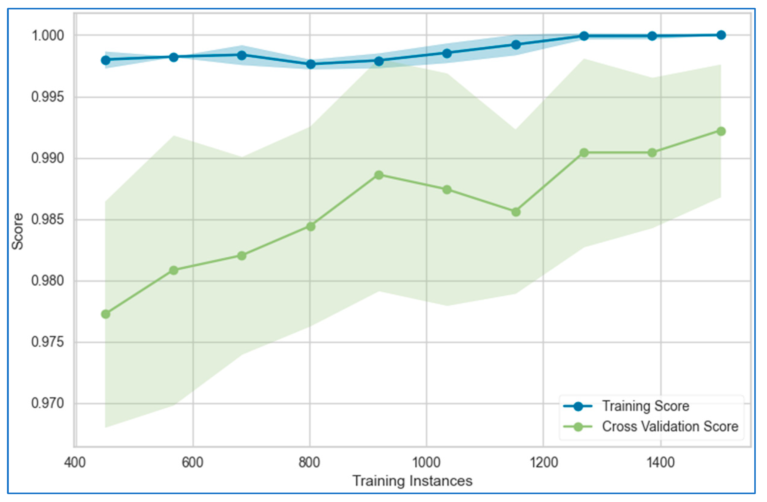
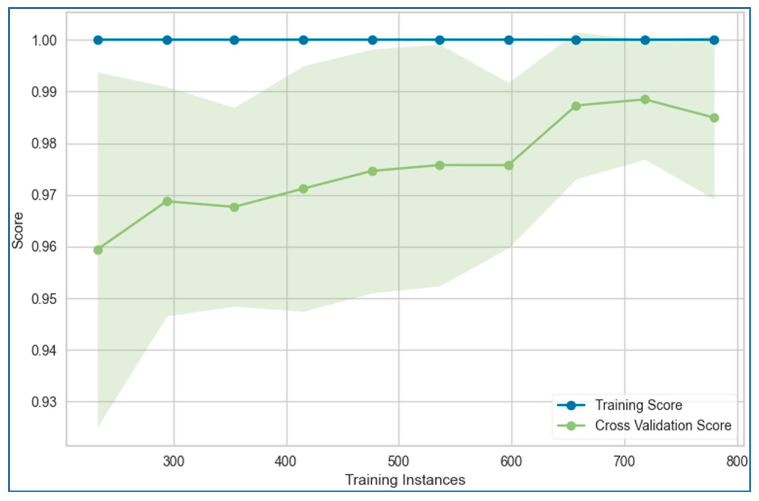
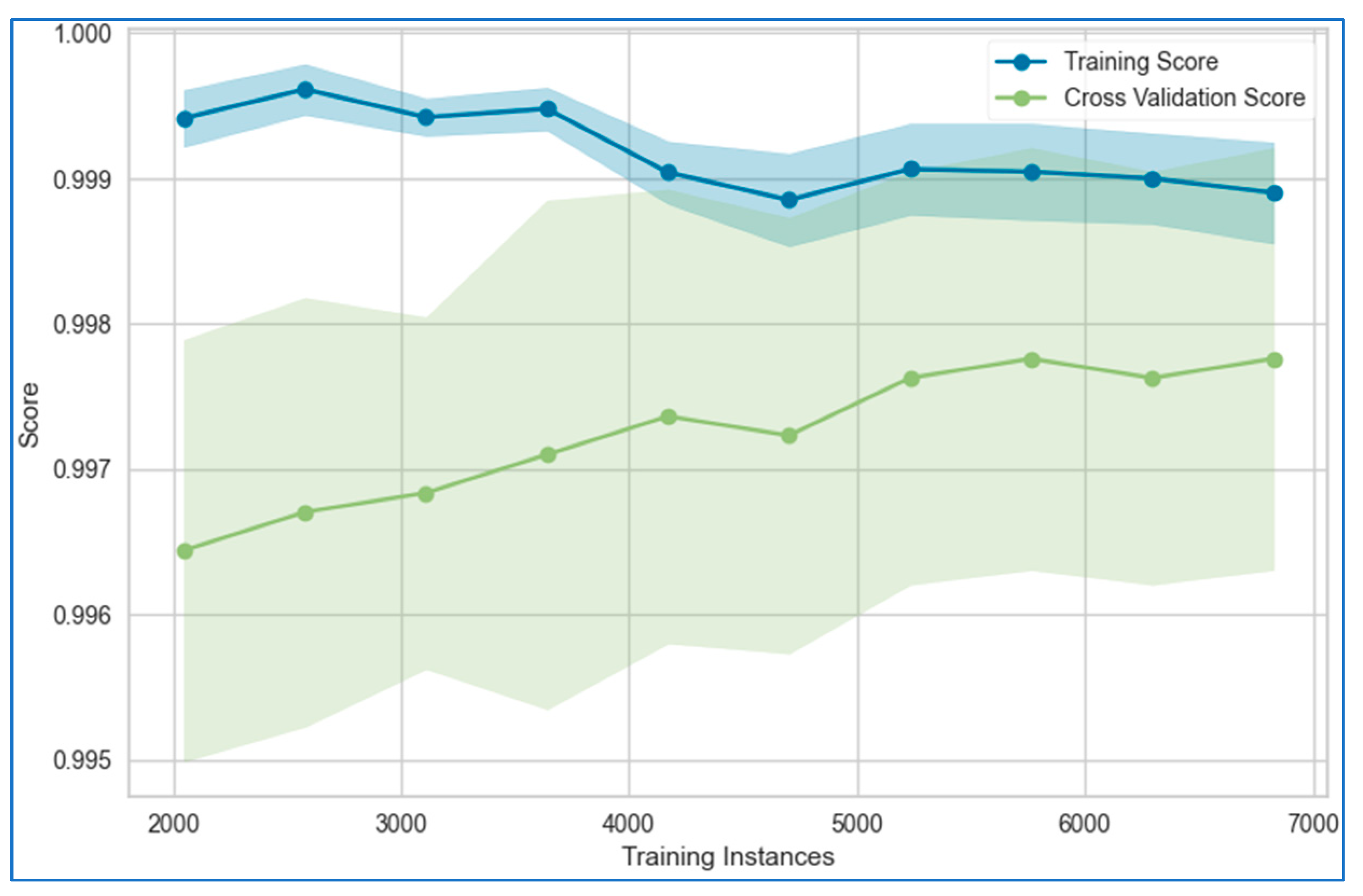
6.1. Learning Curves
6.2. XAI
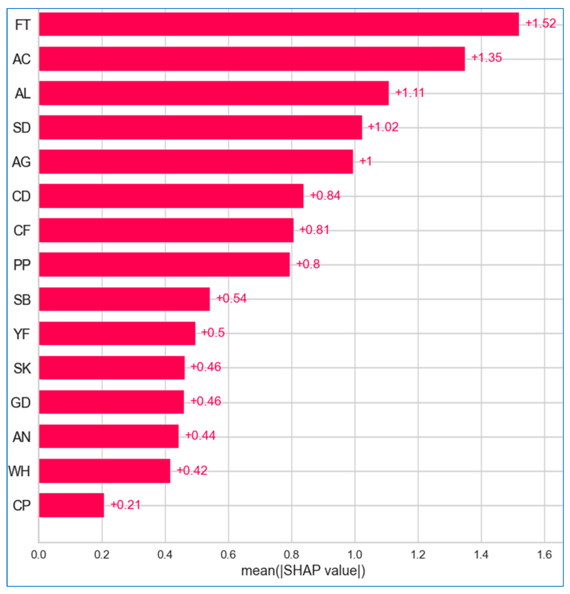
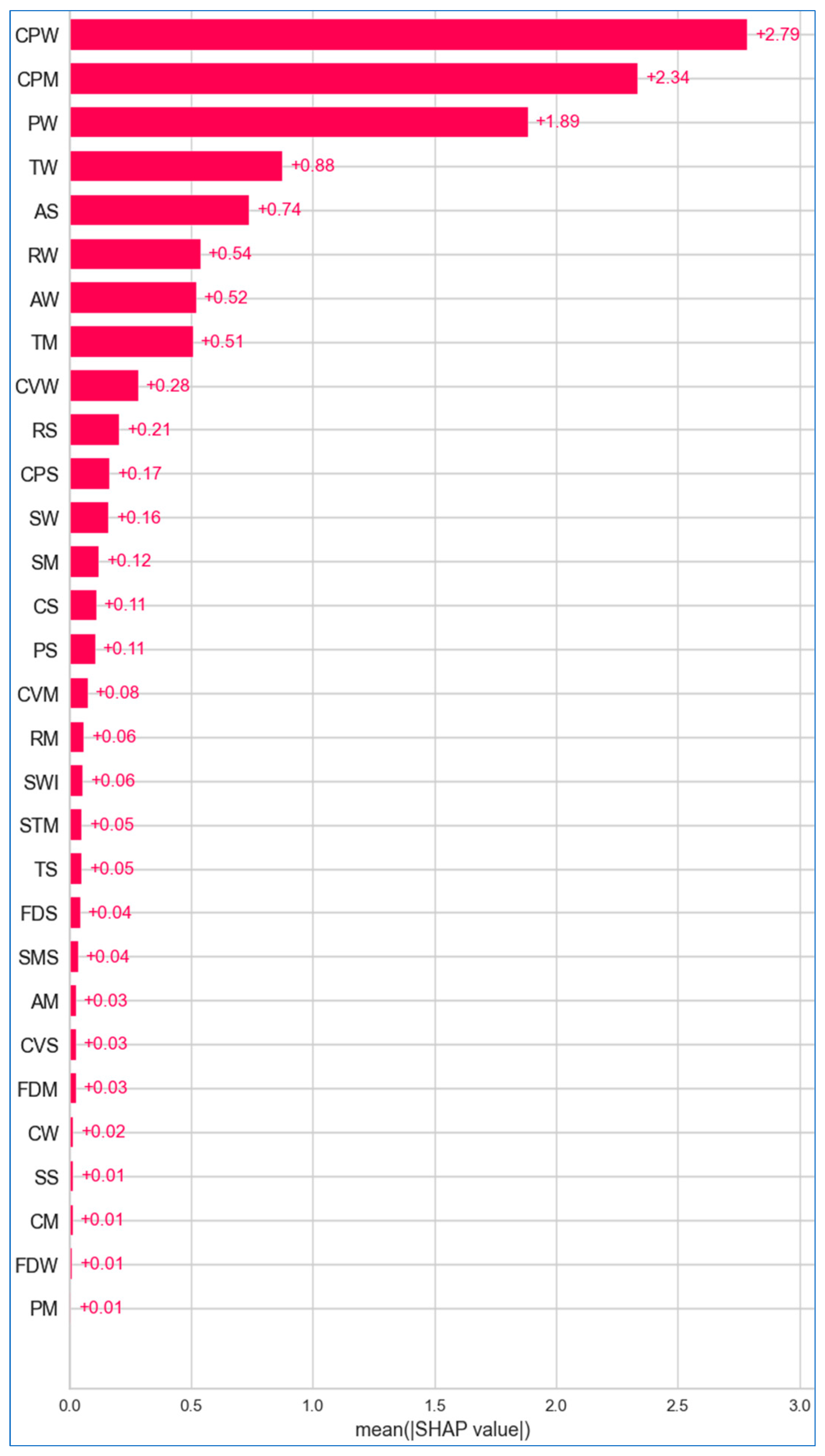
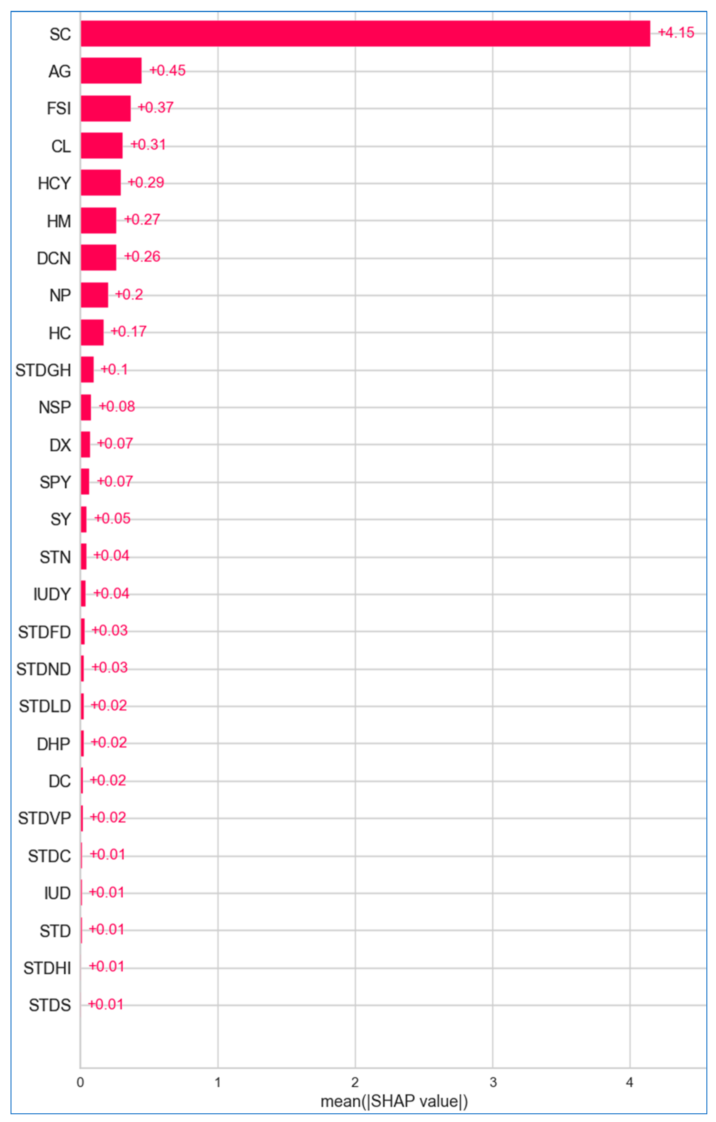
6.2.1. Global Explanation
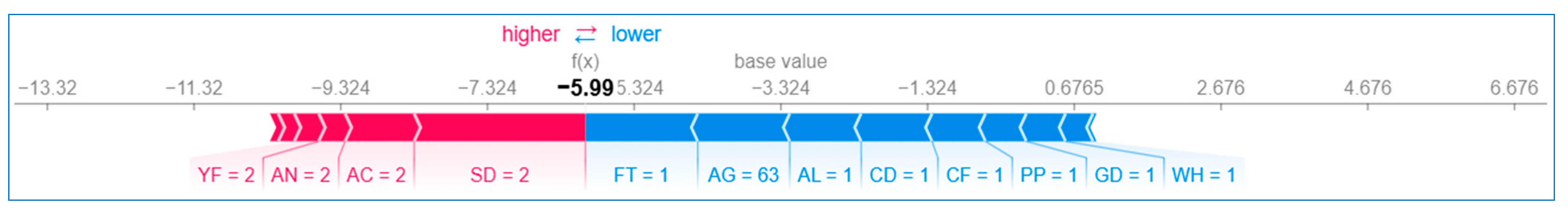
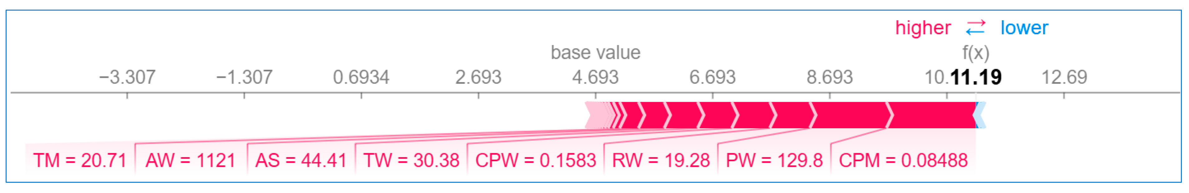
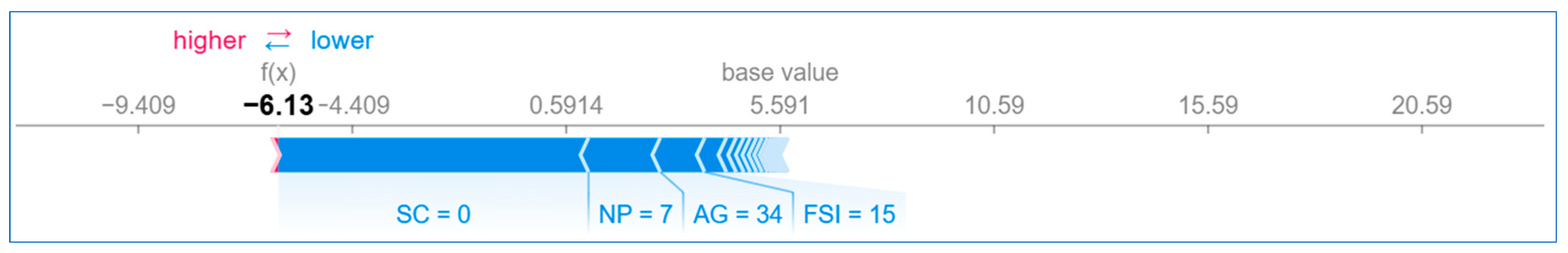
6.2.2. Local Explanation
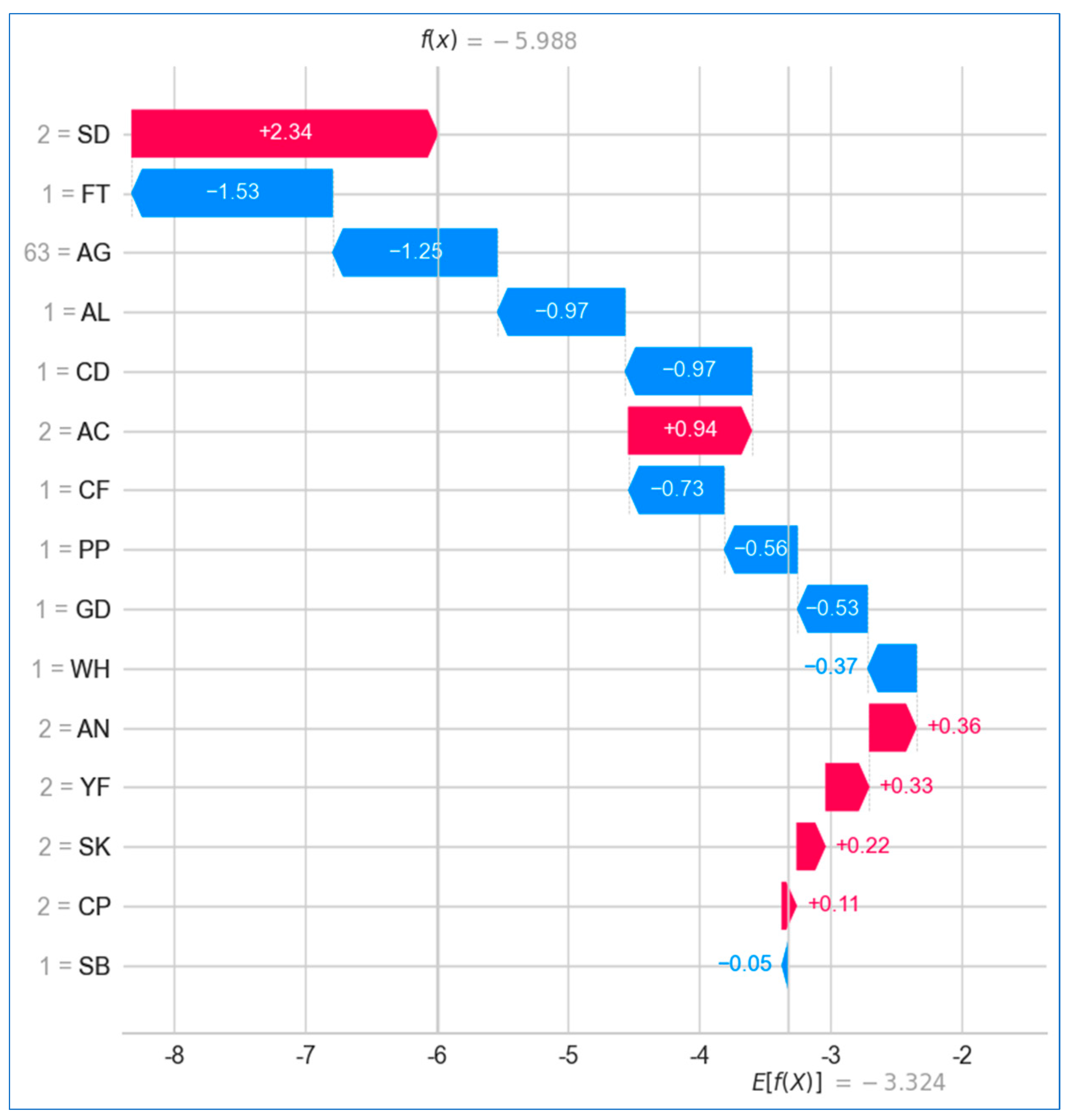
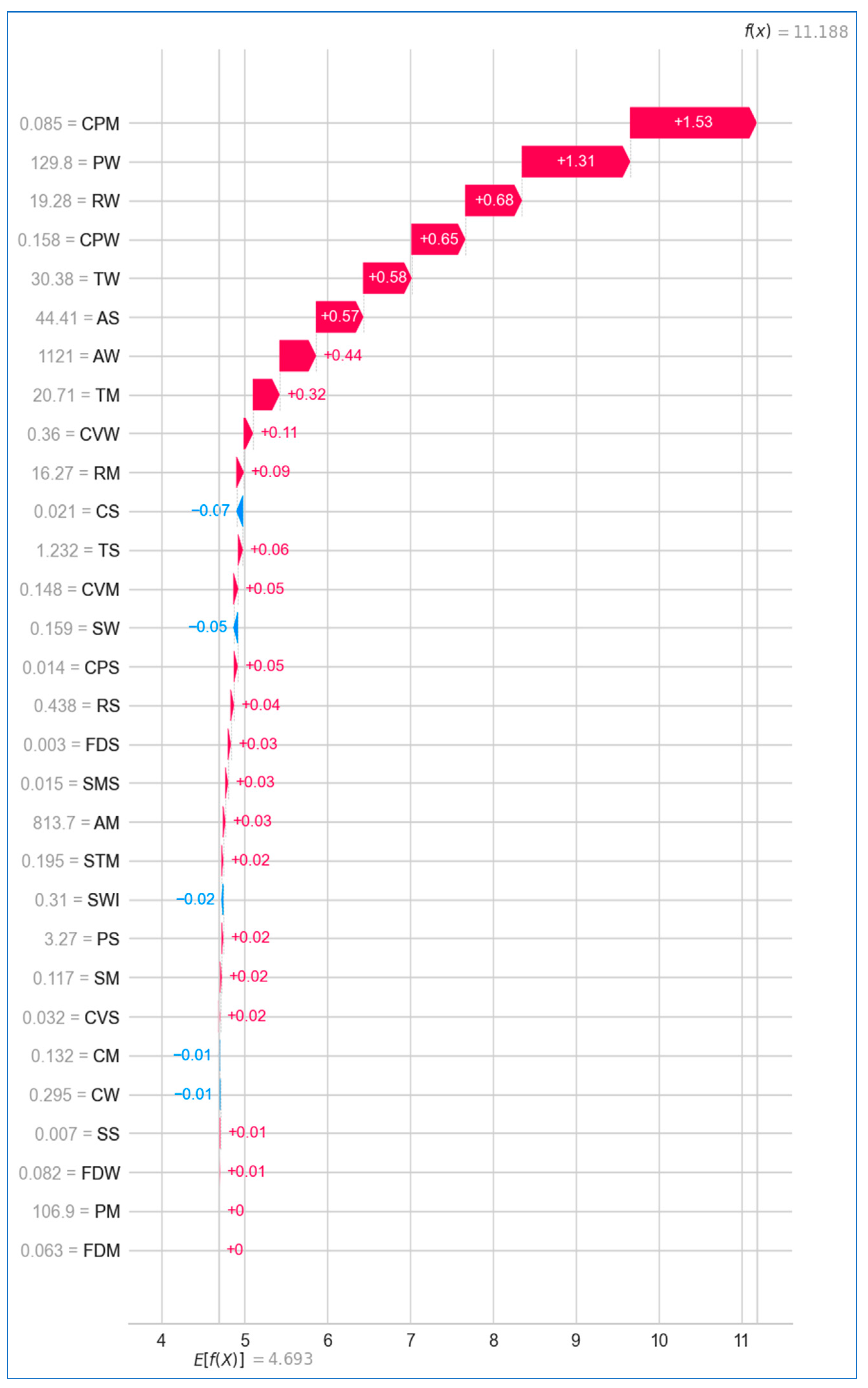
Using Waterfall Plot
Using Force Plot
7. Conclusions, Limitations, and Further Scope
Author Contributions
Funding
Institutional Review Board Statement
Informed Consent Statement
Data Availability Statement
Conflicts of Interest
References
- World Health Organization. Cancer. 3 February 2022. Available online: https://www.who.int/news-room/fact-sheets/detail/cancer (accessed on 4 November 2022).
- Nair, M.; Sandhu, S.S.; Sharma, A.K. Cancer molecular markers: A guide to cancer detection and management. Semin. Cancer Biol. 2018, 52, 39–55. [Google Scholar] [CrossRef] [PubMed]
- Ganie, S.M.; Pramanik, P.K.D. Predicting Chronic Liver Disease Using Boosting Technique. In Proceedings of the International Conference on Artificial Intelligence for Innovations in Healthcare Industries (ICAIIHI), Raipur, India, 29–30 December 2023. [Google Scholar]
- Savarraj, J.P.J.; Hergenroeder, G.W.; Zhu, L.; Chang, T.; Park, S.; Megjhani, M.; Vahidy, F.S.; Zhao, Z.; Kitagawa, R.S.; Choi, H.A. Machine Learning to Predict Delayed Cerebral Ischemia and Outcomes in Subarachnoid Hemorrhage. Neurology 2021, 96, e553–e562. [Google Scholar] [CrossRef]
- Ganie, S.M.; Pramanik, P.K.D.; Mallik, S.; Zhao, Z. Chronic Kidney Disease Prediction Using Boosting Techniques. PLoS ONE 2023, 18, e0295234. [Google Scholar] [CrossRef]
- Ganie, S.M.; Pramanik, P.K.D.; Malik, M.B.; Mallik, S.; Qin, H. An Ensemble Learning Approach for Diabetes Prediction Using Boosting Techniques. Front. Genet. 2023, 13, 1252159. [Google Scholar] [CrossRef]
- Ganie, S.M.; Pramanik, P.K.D.; Malik, M.B.; Nayyar, A.; Kwak, K.S. An Improved Ensemble Learning Approach for Heart Disease Prediction Using Boosting Algorithms. Comput. Syst. Sci. Eng. 2023, 46, 3993–4006. [Google Scholar] [CrossRef]
- Ganie, S.M.; Pramanik, P.K.D.; Zhao, Z. Improved liver disease prediction from clinical data through anevaluation of ensemble learning approaches. BMC Med. Inform. Decis. Mak. 2024, 24, 160. [Google Scholar] [CrossRef]
- Ganie, S.M.; Pramanik, P.K.D. A comparative analysis of boosting algorithms for chronic liver disease prediction. Healthc. Anal. 2024, 5, 100313. [Google Scholar] [CrossRef]
- Ganie, S.M.; Pramanik, P.K.D.; Zhao, Z. Ensemble learning with explainable AI for improved heart disease prediction based on multiple datasets. Sci. Rep. 2025, 15, 13912. [Google Scholar] [CrossRef] [PubMed]
- Molnar, C. Interpretable Machine Learning: A Guide for Making Black Box Models Explainable; LeanPub: Victoria, BC, Canada, 2020. [Google Scholar]
- Nasarian, E.; Alizadehsani, R.; Acharya, U.R.; Tsui, K.-L. Designing interpretable ML system to enhance trust in healthcare: A systematic review to proposed responsible clinician-AI-collaboration framework. Inf. Fusion 2024, 108, 102412. [Google Scholar] [CrossRef]
- Abdullah, D.M.; Abdulazeez, A.M.; Sallow, A.B. Lung Cancer Prediction and Classification Based on Correlation Selection method Using Machine Learning Techniques. Qubahan Acad. J. 2021, 1, 141–149. [Google Scholar] [CrossRef]
- Patra, R. Prediction of Lung Cancer Using Machine Learning Classifier. In Computing Science, Communication and Security (COMS2 2020); Communications in Computer and Information Science; Chaubey, N., Parikh, S., Amin, K., Eds.; Springer: Singapore, 2020; Volume 1235, pp. 132–142. [Google Scholar]
- Islam, M.; Haque, R.; Iqbal, H.; Hasan, M.; Hasan, M.; Kabir, M.N. Breast Cancer Prediction: A Comparative Study Using Machine Learning Techniques. SN Comput. Sci. 2020, 1, 290. [Google Scholar] [CrossRef]
- Yadav, R.K.; Singh, P.; Kashtriya, P. Diagnosis of Breast Cancer Using Machine Learning Techniques—A Survey. Procedia Comput. Sci. 2023, 218, 1434–1443. [Google Scholar] [CrossRef]
- Rawat, P.; Bajaj, M.; Mehta, S.; Sharma, V.; Vats, S. A Study on Cervical Cancer Prediction Using Various Machine Learning Approaches. In Proceedings of the International Conference on Innovative Data Communication Technologies and Application (ICIDCA), Uttarakhand, India, 14–15 March 2023. [Google Scholar]
- Akter, L.; Ferdib-Al-Islam; Islam, M.M.; Al-Rakhami, M.S.; Haque, M.R. Prediction of Cervical Cancer from Behavior Risk Using Machine Learning Techniques. SN Comput. Sci. 2021, 2, 177. [Google Scholar] [CrossRef]
- Das, A.; Mohanty, M.N.; Mallick, P.K.; Tiwari, P.; Muhammad, K.; Zhu, H. Breast cancer detection using an ensemble deep learning method. Biomed. Signal Process. Control 2021, 70, 103009. [Google Scholar] [CrossRef]
- Nemade, V.; Fegade, V. Machine Learning Techniques for Breast Cancer Prediction. Procedia Comput. Sci. 2023, 218, 1314–1320. [Google Scholar] [CrossRef]
- Senthilkumar, B.; Zodinpuii, D.; Pachuau, L.; Chenkual, S.; Zohmingthanga, J.; Kumar, N.S.; Hmingliana, L. Ensemble Modelling for Early Breast Cancer Prediction from Diet and Lifestyle. IFAC Pap. 2022, 55, 429–435. [Google Scholar] [CrossRef]
- Reshan, M.S.A.; Amin, S.; Zeb, M.A.; Sulaiman, A.; Alshahrani, H.; Azar, A.T.; Shaikh, A. Enhancing Breast Cancer Detection and Classification Using Advanced Multi-Model Features and Ensemble Machine Learning Techniques. Life 2023, 13, 2093. [Google Scholar] [CrossRef] [PubMed]
- Uddin, K.M.M.; Mamun, A.A.; Chakrabarti, A.; Mostafiz, R.; Dey, S.K. An ensemble machine learning-based approach to predict cervical cancer using hybrid feature selection. Neurosci. Inform. 2024, 4, 100169. [Google Scholar] [CrossRef]
- Ali, M.S.; Hossain, M.M.; Kona, M.A.; Nowrin, K.R.; Islam, M. An ensemble classification approach for cervical cancer prediction using behavioral risk factors. Healthc. Anal. 2024, 5, 100324. [Google Scholar] [CrossRef]
- Ahmad, A.S.; Mayya, A.M. A new tool to predict lung cancer based on risk factors. Heliyon 2020, 6, e03402. [Google Scholar] [CrossRef]
- Safiyari, A.; Javidan, R. Predicting lung cancer survivability using ensemble learning methods. In Proceedings of the Intelligent Systems Conference (IntelliSys), London, UK, 7–8 September 2017. [Google Scholar]
- Wang, Q.; Zhou, Y.; Ding, W.; Zhang, Z.; Muhammad, K.; Cao, Z. Random forest with self-paced bootstrap learning in lung cancer prognosis. ACM Trans. Multimed. Comput. Commun. Appl. 2020, 16, 1–12. [Google Scholar] [CrossRef]
- Siddhartha, M.; Maity, P.; Nath, R. Explanatory Artificial Intelligence (XAI) In The Prediction of Post-Operative Life Expectancy in Lung Cancer Patients. Int. J. Sci. Res. 2019, VIII, 23–28. [Google Scholar]
- Mamun, M.; Farjana, A.; Mamun, M.A.; Ahammed, M.S. Lung cancer prediction model using ensemble learning techniques and a systematic review analysis. In Proceedings of the IEEE World AI IoT Congress (AIIoT), Seattle, DC, USA, 6–9 June 2022. [Google Scholar]
- Jaiswal, V.; Saurabh, P.; Lilhore, U.K.; Pathak, M.; Simaiya, S.; Dalal, S. A breast cancer risk predication and classification model with ensemble learning and big data fusion. Decis. Anal. J. 2023, 8, 100298. [Google Scholar] [CrossRef]
- Rabiei, R.; Ayyoubzadeh, S.M.; Sohrabei, S.; Esmaeili, M.; Atashi, A. Prediction of Breast Cancer Using Machine Learning Approaches. J. Biomed. Phys. Eng. 2022, 12, 297–308. [Google Scholar] [CrossRef] [PubMed]
- Naji, M.A.; Filali, S.E.; Aarika, K.; Benlahmar, E.H.; Abdelouhahid, R.A.; Debauche, O. Machine Learning Algorithms for Breast Cancer Prediction and Diagnosis. Procedia Comput. Sci. 2012, 191, 487–492. [Google Scholar] [CrossRef]
- Liu, P.; Fu, B.; Yang, S.X.; Deng, L.; Zhong, X.; Zheng, H. Optimizing Survival Analysis of XGBoost for Ties to Predict Disease Progression of Breast Cancer. IEEE Trans. Biomed. Eng. 2021, 68, 148–160. [Google Scholar] [CrossRef] [PubMed]
- Alam, T.M.; Khan, M.M.A.; Iqbal, M.A.; Abdul, W.; Mushtaq, M. Cervical Cancer Prediction Through Different Screening Methods Using Data Mining. Int. J. Adv. Comput. Sci. Appl. 2019, 10, 388–396. [Google Scholar] [CrossRef]
- Lu, J.; Ghoneim, A.; Alrashoud, M. Machine learning for assisting cervical cancer diagnosis: An ensemble approach. Future Gener. Comput. Syst. 2020, 106, 199–205. [Google Scholar] [CrossRef]
- Jahan, S.; Islam, M.D.S.; Islam, L.; Rashme, T.Y.; Prova, A.A.; Paul, B.K.; Islam, M.D.M.; Mosharof, M.K. Automated invasive cervical cancer disease detection at early stage through suitable machine learning model. SN Appl. Sci. 2021, 3, 806. [Google Scholar] [CrossRef]
- Alsmariy, R.; Healy, G.; Hoda, A. Predicting Cervical Cancer Using Machine Learning Methods. Int. J. Adv. Comput. Sci. Appl. 2020, 11, 173–184. [Google Scholar] [CrossRef]
- Zhang, S.; Yang, L.; Xu, W.; Wang, Y.; Han, L.; Zhao, G.; Cai, T. Predicting the risk of lung cancer using machine learning: A large study based on UK Biobank. Medicine 2024, 103, e37879. [Google Scholar] [CrossRef] [PubMed]
- Aravena, F.S.; Delafuente, H.N.; Bahamondes, J.H.G.; Morales, J. A Hybrid Algorithm of ML and XAI to Prevent Breast Cancer: A Strategy to Support Decision Making. Cancers 2023, 15, 2443. [Google Scholar] [CrossRef] [PubMed]
- Makubhai, S.S.; Pathak, G.R.; Chandre, P.R. Predicting lung cancer risk using explainable artificial. Bull. Electr. Eng. Inform. 2024, 13, 1276–1285. [Google Scholar] [CrossRef]
- McCallum, A.; Nigam, K. A comparison of event models for naive bayes text classification. AAAI-98 Workshop Learn. Text Categ. 1998, 752, 41–48. [Google Scholar]
- Schapire, R.E.; Singer, Y. Improved Boosting Algorithms Using Confidence-Rated Predictions. Mach. Learn. 1999, 37, 297–336. [Google Scholar] [CrossRef]
- Ghosh, A.; SahaRay, R.; Chakrabarty, S.; Bhadra, S. Robust generalised quadratic discriminant analysis. Pattern Recognit. 2021, 117, 107981. [Google Scholar] [CrossRef]
- Nouretdinov, I.; Melluish, T.; Vovk, V. Ridge Regression Confidence Machine. In Proceedings of the Eighteenth International Conference on Machine Learning (ICML ‘01), Williamstown, MA, USA, 28 June–1 July 2001. [Google Scholar]
- Cover, T.; Hart, P.E. Nearest neighbor pattern classification. IEEE Trans. Inf. Theory 1967, 13, 21–27. [Google Scholar] [CrossRef]
- Hart, P.E.; Stork, D.G.; Duda, R.O. Pattern Classification, 2nd ed.; John Wiley & Sons: Hoboken, NJ, USA, 2000. [Google Scholar]
- Hastie, T.; Tibshirani, R.; Friedman, J. The Elements of Statistical Learning: Data Mining, Inference, and Prediction; Springer: Berlin/Heidelberg, Germany, 2009. [Google Scholar]
- Freund, Y.; Schapire, R.E. A Decision-Theoretic Generalization of On-Line Learning and an Application to Boosting. J. Comput. Syst. Sci. 1997, 55, 119–139. [Google Scholar] [CrossRef]
- Aziz, N.; Akhir, E.A.P.; Aziz, I.A.; Jaafar, J.; Hasan, M.H.; Abas, A.N.C. A study on gradient boosting algorithms for development of AI monitoring and prediction systems. In Proceedings of the International Conference on Computational Intelligence (ICCI), Bandar Seri Iskandar, Malaysia, 8–9 October 2020. [Google Scholar]
- Freund, Y.; Schapire, R.E. A Short Introduction to Boosting. J. Jpn. Soc. Artif. Intell. 1999, 14, 771–780. [Google Scholar]
- Breiman, L. Random forests. Mach. Learn. 2001, 45, 5–32. [Google Scholar] [CrossRef]
- Geurts, P.; Ernst, D.; Wehenkel, L. Extremely randomized trees. Mach. Learn. 2006, 63, 3–42. [Google Scholar] [CrossRef]
- Blagus, R.; Lusa, L.; Bioinformatics, B.M. SMOTE for high-dimensional class-imbalanced data. BMC Bioinform. 2013, 14, 106. [Google Scholar] [CrossRef] [PubMed]
- Hairani, H.; Widiyaningtyas, T.; Prasetya, D.D. Addressing Class Imbalance of Health Data: A Systematic Literature Review on Modified Synthetic Minority Oversampling Technique (SMOTE) Strategies. Int. J. Inform. Vis. 2024, 8, 1310–1318. [Google Scholar] [CrossRef]
- Kivrak, M.; Avci, U.; Uzun, H.; Ardic, C. The Impact of the SMOTE Method on Machine Learning and Ensemble Learning Performance Results in Addressing Class Imbalance in Data Used for Predicting Total Testosterone Deficiency in Type 2 Diabetes Patients. Diagnostics 2024, 14, 2634. [Google Scholar] [CrossRef]
- Radhika, P.R.; Rakhi, A.S.N.; Veena, G. A Comparative Study of Lung Cancer Detection Using Machine Learning Algorithms. In Proceedings of the IEEE International Conference on Electrical, Computer and Communication Technologies (ICECCT), Coimbatore, India, 20–22 February 2019. [Google Scholar]
- Lundberg, S.M.; Lee, S.-I. A unified approach to interpreting model predictions. In Proceedings of the 31st International Conference on Neural Information Processing Systems, Long Beach, CA, USA, 4–9 December 2017. [Google Scholar]


| Abbreviation | Full Name | Abbreviation | Full Name |
|---|---|---|---|
| ADB | AdaBoost | LCPT | Lung cancer prediction tool |
| AUC | Area under the curve | LDA | Linear discriminant analysis |
| AUPRC | Area under precision–recall curve | LGBM | Light gradient boosting machine |
| BCWD | Breast cancer Wisconsin (diagnostic) | LR | Logistic regression |
| BDT | Boosted decision tree | MB | Multi boosting |
| BME | Bagging meta-estimator | MCC | Matthews correlation coefficient |
| BRF | Balanced random forest | MLP | Multilayer perceptron |
| BSPL | Bootstrap with self-paced learning | NB | Naive Bayes |
| CB | Cat boosting | NCC | Nearest centroid classifier |
| CCrf | Cervical cancer (risk factors) | PCA | Principal component analysis |
| CNN | Convolutional neural network | PDP | Partial dependence plots |
| CRCB | Clinical research center for breast | RBF | Radial basis function |
| DF | Decision forest | RF | Random forest |
| DJ | Decision jungle | RFE | Recursive feature elimination |
| DNN | Deep neural network | ROC | Receiver operating characteristic |
| DT | Decision tree | RSF | Random survival forest |
| ERT | Extremely randomized trees | SD | Standard deviation |
| ET | Extra trees | SEER | Surveillance, epidemiology, and end results |
| EXSA | Extended XGB for survival analysis | SHAP | Shapley additive explanations |
| FN | False negative | SMO | Sequential minimal optimization |
| FP | False positive | STD | Sexually transmitted diseases |
| FPR | False positive rate | SVM | Support vector machine |
| GB | Gradient boosting | TN | True negative |
| IQR | Interquartile range | TP | True positive |
| IUD | Intrauterine device | WDBC | Wisconsin diagnostic breast cancer |
| KNN | K-nearest neighbor | XGB | Extreme gradient boosting |
| Metric | Significance and Interpretation | Calculation |
|---|---|---|
| Accuracy | Accuracy represents the proportion of correct predictions (both true positives and true negatives) out of the total number of predictions. It provides an overall measure of the model’s ability to correctly identify both cancer and non-cancer cases. A high accuracy indicates that the model is performing well, but it may not be the best metric in cases where the data are imbalanced. | |
| Precision | Precision measures the proportion of true positive predictions out of all the positive predictions made by the model. It reflects the model’s ability to correctly identify cancer cases without falsely labeling non-cancer cases as cancer. A high precision is crucial in cancer screening to avoid unnecessary further testing or treatment. | |
| Recall | Recall, also known as sensitivity, represents the proportion of true positive predictions out of all the actual cancer cases. It reflects the model’s ability to correctly identify cancer cases. A high recall is important in cancer diagnosis to ensure that the model does not miss any cancer cases. | |
| F1-score | The F1-score is the harmonic mean of precision and recall, providing a balanced measure of the model’s performance. It is particularly useful when the data are imbalanced, as it considers both the model’s ability to correctly identify cancer cases and its ability to avoid false positives. | |
| MCC | MCC is a more comprehensive performance metric that considers all four confusion matrix elements (true positives, true negatives, false positives, and false negatives). It provides a balanced measure of the model’s performance, ranging from −1 to 1, where 1 indicates a perfect prediction, 0 indicates a random prediction, and −1 indicates a completely inverse prediction. | |
| Kappa | Cohen’s Kappa is a statistical measure that evaluates the model’s performance while considering the possibility of chance agreement. It is particularly useful when the data are imbalanced, as it takes into account the expected agreement by chance. Kappa values range from −1 to 1, with 1 indicating perfect agreement, 0 indicating agreement no better than chance, and negative values indicating agreement worse than chance. | |
| ROC curve | The ROC curve is a plot of the true positive rate (sensitivity) against the false positive rate (1—specificity) at various classification thresholds. It provides a visual representation of the trade-off between sensitivity and specificity, allowing you to evaluate the model’s performance across different decision boundaries. | Recall (y axis) vs. FPR (x axis) |
| AUC | The AUC of the ROC curve represents the probability that a randomly selected cancer case will be ranked higher than a randomly selected non-cancer case by the model. It ranges from 0 to 1, with 1 indicating a perfect model and 0.5 indicating a random model. A higher AUC value indicates better overall diagnostic performance. | , t is a threshold |
| Parameter | Description | Measurement | Mean | Std | Min | Max |
|---|---|---|---|---|---|---|
| Demographic and lifestyle parameters | ||||||
| Gender (GD) | The gender of the individual | Male/female | 0.48 | 0.50 | 0 | 1 |
| Age (AG) | The age of the individual | Numeric | 61.96 | 8.63 | 21 | 87 |
| Smoking (SK) | Whether the individual is or has been a smoker. | Yes (2)/no (1) | 1.54 | 0.49 | 1 | 2 |
| Alcohol consuming (AC) | Whether the individual consumes alcohol. | Yes (2)/no (1) | 1.40 | 0.49 | 1 | 2 |
| Yellow fingers (YF) | Whether the individual has yellowed fingers, often associated with long-term smoking. | Yes (2)/no (1) | 1.47 | 0.49 | 1 | 2 |
| Psychological and social influence factors | ||||||
| Anxiety (AN) | Whether the individual suffers from anxiety. | Yes (2)/no (1) | 1.42 | 0.49 | 1 | 2 |
| Peer pressure (PP) | Whether the individual feels influenced by peers to engage in risky behaviors like smoking. | Yes (2)/no (1) | 1.39 | 0.48 | 1 | 2 |
| Health and symptom-related parameters | ||||||
| Chronic disease (CD) | Whether the individual has any chronic disease. | Yes (2)/no (1) | 1.44 | 0.49 | 1 | 2 |
| Fatigue (FT) | Whether the individual experiences fatigue. | Yes (2)/no (1) | 1.58 | 0.49 | 1 | 2 |
| Allergy (AL) | Whether the individual has allergies. | Yes (2)/no (1) | 1.38 | 0.48 | 1 | 2 |
| Wheezing (WH) | Whether the individual experiences wheezing, which is a high-pitched whistling sound when breathing. | Yes (2)/no (1) | 1.40 | 0.49 | 1 | 2 |
| Coughing (CF) | Whether the individual experiences persistent coughing. | Yes (2)/no (1) | 1.43 | 0.49 | 1 | 2 |
| Shortness of breath (SB) | Whether the individual experiences shortness of breath. | Yes (2)/no (1) | 1.60 | 0.48 | 1 | 2 |
| Swallowing difficulty (SD) | Whether the individual has trouble swallowing. | Yes (2)/no (1) | 1.32 | 0.46 | 1 | 2 |
| Chest pain (CP) | Whether the individual experiences chest pain. | Yes (2)/no (1) | 1.43 | 0.49 | 1 | 2 |
| Target variable | ||||||
| Lung cancer (LC) | Whether the individual has been diagnosed with lung cancer. | Yes (2)/no (1) | 0.50 | 0.50 | 0 | 1 |
| Parameter | Description | Measurement | Mean | Std | Min | Max |
|---|---|---|---|---|---|---|
| Mean values (computed on the mean of all cells in the image) | ||||||
| Radius_mean (RM) | The mean radius of the cell nuclei, which is the average distance from the center to the boundary of the nucleus. | Decimal | 14.12729 | 3.524049 | 6.981 | 28.11 |
| Texture_mean (TM) | The mean standard deviation of the gray-scale values in the image, which measures the smoothness or roughness of the cell nuclei | Decimal | 19.28965 | 4.301036 | 9.71 | 39.28 |
| Perimeter_mean (PM) | The mean perimeter of the cell nuclei, representing the boundary length. | Decimal | 91.96903 | 24.29898 | 43.79 | 188.5 |
| Area_mean (AM) | The mean area of the cell nuclei, indicating the size of the nuclei. | Decimal | 654.8891 | 351.9141 | 143.5 | 2501 |
| Smoothness_mean (SM) | The mean measure of how smooth the edges of the nuclei are, calculated as the variation in radius lengths. | Decimal | 0.09636 | 0.014064 | 0.05263 | 0.1634 |
| Compactness_mean (CM) | The mean measure of how compact the nuclei are, computed as PM2/AM, indicating the roundness of the nuclei. | Decimal | 0.104341 | 0.052813 | 0.01938 | 0.3454 |
| Concavity_mean (CVM) | The mean extent of concave portions of the nucleus boundary. | Decimal | 0.088799 | 0.07972 | 0 | 0.4268 |
| Concave points_mean (CPM) | The mean number of concave points on the nucleus boundary. | Decimal | 0.048919 | 0.038803 | 0 | 0.2012 |
| Symmetry_mean (SM) | The mean symmetry of the nucleus, measuring how symmetrical the nucleus shape is. | Decimal | 0.181162 | 0.027414 | 0.106 | 0.304 |
| Fractal_dimension_mean (FDM) | The mean fractal dimension of the nucleus, which indicates the complexity of the nucleus boundary (calculated as “coastline approximation”). | Decimal | 0.062798 | 0.00706 | 0.04996 | 0.09744 |
| Standard error values (measure of uncertainty/variation in each feature) | ||||||
| Radius_se (RS) | The standard error of the radius of the cell nuclei. | Decimal | 0.405172 | 0.277313 | 0.1115 | 2.873 |
| Texture_se (TS) | The standard error of the texture, indicating variability in gray-scale intensity. | Decimal | 1.216853 | 0.551648 | 0.3602 | 4.885 |
| Perimeter_se (PS) | The standard error of the perimeter of the cell nuclei. | Decimal | 2.866059 | 2.021855 | 0.757 | 21.98 |
| Area_se (AS) | The standard error of the area of the cell nuclei. | Decimal | 40.33708 | 45.49101 | 6.802 | 542.2 |
| Smoothness_se (SS) | The standard error of the smoothness. | Decimal | 0.007041 | 0.003003 | 0.001713 | 0.03113 |
| Compactness_se (CS) | The standard error of the compactness. | Decimal | 0.025478 | 0.017908 | 0.002252 | 0.1354 |
| Concavity_se (CVS) | The standard error of the concavity. | Decimal | 0.031894 | 0.030186 | 0 | 0.396 |
| Concave points_se (CPS) | The standard error of the concave points. | Decimal | 0.011796 | 0.00617 | 0 | 0.05279 |
| Symmetry_se (SMS) | The standard error of the symmetry. | Decimal | 0.020542 | 0.008266 | 0.007882 | 0.07895 |
| Fractal_dimension_se (FDS) | The standard error of the fractal dimension. | Decimal | 0.003795 | 0.002646 | 0.000895 | 0.02984 |
| “Worst” values (largest values for each feature) | ||||||
| Radius_worst (RW) | The largest radius observed among all cell nuclei in the image. | Decimal | 16.26919 | 4.833242 | 7.93 | 36.04 |
| Texture_worst (TW) | The largest texture value observed. | Decimal | 25.67722 | 6.146258 | 12.02 | 49.54 |
| Perimeter_worst (PW) | The largest perimeter value observed. | Decimal | 107.2612 | 33.60254 | 50.41 | 251.2 |
| Area_worst (AW) | The largest area observed among the nuclei. | Decimal | 880.5831 | 569.357 | 185.2 | 4254 |
| Smoothness_worst (SW) | The worst (largest) value of smoothness observed. | Decimal | 0.132369 | 0.022832 | 0.07117 | 0.2226 |
| Compactness_worst (CW) | The largest compactness value observed. | Decimal | 0.254265 | 0.157336 | 0.02729 | 1.058 |
| Concavity_worst (CVW) | The largest concavity value observed. | Decimal | 0.272188 | 0.208624 | 0 | 1.252 |
| Concave points_worst (CPW) | The largest number of concave points observed. | Decimal | 0.114606 | 0.065732 | 0 | 0.291 |
| Symmetry_worst (SWI) | The worst (largest) symmetry value. | Decimal | 0.290076 | 0.061867 | 0.1565 | 0.6638 |
| Fractal_dimension_worst (FDW) | The largest fractal dimension observed. | Decimal | 0.083946 | 0.018061 | 0.05504 | 0.2075 |
| Target variable | ||||||
| Diagnosis (BC) | This is the target variable, indicating whether the tumor is benign or malignant. It represents the classification of the tumor based on the features described above. | 1 (yes)/0 (no) | 0.372583 | 0.483918 | 0 | 1 |
| Parameter | Description | Measurement | Mean | Std | Min | Max |
|---|---|---|---|---|---|---|
| Demographic and sexual behavior parameters | ||||||
| Age (AG) | The age of the patient. | Numeric | 27.02395 | 8.482986 | 13 | 84 |
| Number of sexual partners (NSP) | The total number of sexual partners the individual has had, which can influence the risk of contracting STDs. | Numeric | 2.535329 | 1.654044 | 1 | 28 |
| First sexual intercourse (FSI) | The age at which the individual had their first sexual intercourse. | Numeric | 17.02036 | 2.805154 | 10 | 32 |
| Num of pregnancies (NP) | The total number of pregnancies the individual has had. | Numeric | 2.283832 | 1.408152 | 0 | 11 |
| Smoking-related parameters | ||||||
| Smokes (SK) | Whether the individual smokes. | Yes (1)/no (0) | 0.147305 | 0.354623 | 0 | 1 |
| Smokes (years) (SY) | The number of years the individual has been smoking. | Numeric | 1.249898 | 4.108449 | 0 | 37 |
| Smokes (packs/year) (SPY) | The number of packs of cigarettes the individual smokes per year. | Numeric | 0.458571 | 2.239363 | 0 | 37 |
| Hormonal contraceptive and IUD use | ||||||
| Hormonal contraceptives (HC) | Whether the individual uses or has used hormonal contraceptives (e.g., birth control pills). | Yes (1)/no (0) | 0.571257 | 0.495193 | 0 | 1 |
| Hormonal contraceptives (years) (HCY) | The number of years the individual has been using hormonal contraceptives. | Numeric | 2.26555 | 3.553566 | 0 | 30 |
| IUD (IUD) | Whether the individual uses or has used an intrauterine device (IUD) for birth control. | Yes (1)/no (0) | 0.099401 | 0.299379 | 0 | 1 |
| IUD (years) (IUDY) | The number of years the individual has been using an IUD, to quantify long-term use. | Numeric | 0.45685 | 1.83754 | 0 | 19 |
| STD-related parameters | ||||||
| STDs (STD) | Whether the individual has had any STDs. | Yes (1)/no (0) | 0.094611 | 0.292852 | 0 | 1 |
| STDs (number) (STN) | The total number of STDs the individual has been diagnosed with. | Numeric | 0.159281 | 0.536236 | 0 | 4 |
| STDs:condylomatosis (STDC) | Whether the individual has been diagnosed with condylomatosis, a type of genital wart caused by certain strains of HPV. | Yes (1)/no (0) | 0.052695 | 0.223557 | 0 | 1 |
| STDs:cervical condylomatosis (STDCC) | A specific condition where condylomatosis affects the cervix. | Yes (1)/no (0) | 0 | 0 | 0 | 0 |
| STDs:vaginal condylomatosis (STDVC) | A condition where condylomatosis affects the vaginal area. | Yes (1)/no (0) | 0.00479 | 0.069088 | 0 | 1 |
| STDs:vulvo-perineal condylomatosis (STDVP) | Condylomatosis affecting the vulva and perineal areas. | Yes (1)/no (0) | 0.051497 | 0.221142 | 0 | 1 |
| STDs:syphilis (STDS) | Whether the individual has had syphilis, another STD that can affect general health and reproductive health. | Yes (1)/no (0) | 0.021557 | 0.145319 | 0 | 1 |
| STDs:pelvic inflammatory disease (STDPI) | Whether the individual has had pelvic inflammatory disease, a complication of STDs that affects the female reproductive organs. | Yes (1)/no (0) | 0.001198 | 0.034606 | 0 | 1 |
| STDs:genital herpes (STDGH) | Whether the individual has had genital herpes, an STD caused by the herpes simplex virus. | Yes (1)/no (0) | 0.001198 | 0.034606 | 0 | 1 |
| STDs:molluscum contagiosum (STDMC) | Whether the individual has been diagnosed with molluscum contagiosum, a viral infection that can be spread sexually. | Yes (1)/no (0) | 0.001198 | 0.034606 | 0 | 1 |
| STDs:AIDS (STDAI) | Whether the individual has been diagnosed with AIDS, a condition caused by HIV that weakens the immune system. | Yes (1)/no (0) | 0 | 0 | 0 | 0 |
| STDs:HIV (STDHI) | Whether the individual is HIV-positive. | Yes (1)/no (0) | 0.021557 | 0.145319 | 0 | 1 |
| STDs:Hepatitis B (STDHB) | Whether the individual has been diagnosed with Hepatitis B, a viral infection that can affect the liver but also has implications for general health. | Yes (1)/no (0) | 0.001198 | 0.034606 | 0 | 1 |
| STDs:HPV (STDHP) | Whether the individual has been diagnosed with HPV (human papillomavirus). | Yes (1)/no (0) | 0.002395 | 0.048912 | 0 | 1 |
| STDs:Number of diagnosis (STDND) | The number of STD diagnoses the individual has received over time. | Numeric | 0.08982 | 0.306335 | 0 | 3 |
| STDs:Time since first diagnosis (STDFD) | The amount of time since the individual’s first STD diagnosis. | Numeric | 6.011976 | 1.70831 | 1 | 22 |
| STDs:Time since last diagnosis (STDLD) | The time since the individual’s most recent STD diagnosis. | Numeric | 5.069461 | 1.682884 | 1 | 22 |
| Diagnosis results | ||||||
| Dx:CIN (DCN) | Whether the individual has been diagnosed with cervical intraepithelial neoplasia (CIN), a pre-cancerous condition in the cervix. | Yes (1)/no (0) | 0.010778 | 0.10332 | 0 | 1 |
| Dx:HPV (DHP) | Whether the individual has been diagnosed with HPV infection. | Yes (1)/no (0) | 0.021557 | 0.145319 | 0 | 1 |
| Dx (DX) | A general diagnostic indicator that may represent additional medical conditions diagnosed. | Yes (1)/no (0) | 0.028743 | 0.167182 | 0 | 1 |
| Screening tests | ||||||
| Hinselmann (HM) | A result from the Hinselmann test, a colposcopy test used to visually examine the cervix for signs of disease, including cancer. | Yes (1)/no (0) | 0.041916 | 0.200518 | 0 | 1 |
| Schiller (SC) | A result from the Schiller test, in which iodine is applied to the cervix to detect abnormalities based on how cells absorb the iodine. | Yes (1)/no (0) | 0.087425 | 0.282626 | 0 | 1 |
| Citology (CL) | A cytological examination of cells (e.g., a Pap smear) used to detect abnormal cells that could indicate precancerous or cancerous changes. | Yes (1)/no (0) | 0.051497 | 0.221142 | 0 | 1 |
| Biopsy (CC) | A biopsy result, which involves the removal of a small sample of cervical tissue to check for cancerous or pre-cancerous changes. | Yes (1)/no (0) | 0.064671 | 0.246091 | 0 | 1 |
| Target variable | ||||||
| Dx:Cancer (DC) | Whether the individual has been diagnosed with cancer. | Yes (1)/no (0) | 0.021557 | 0.145319 | 0 | 1 |
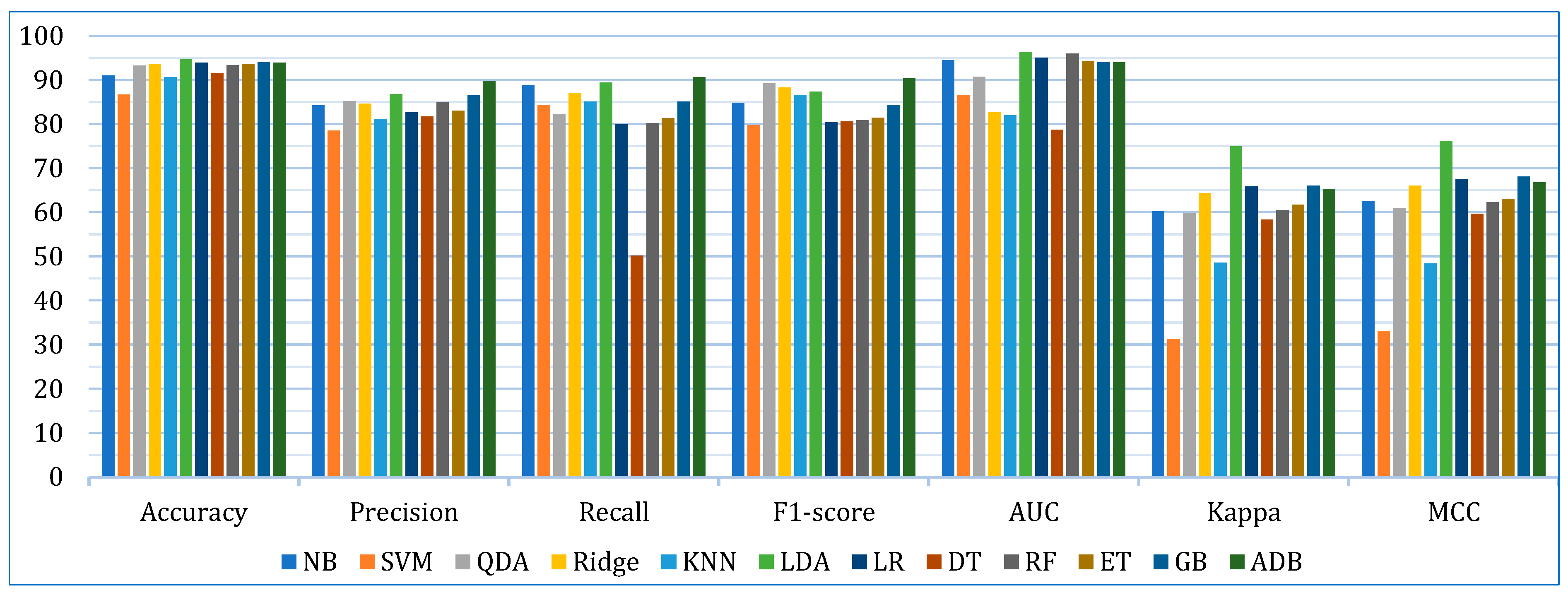
| Metric | Dataset | NB | SVM | QDA | Ridge | KNN | LDA | LR | DT | RF | ET | GB | ADB |
|---|---|---|---|---|---|---|---|---|---|---|---|---|---|
| Accuracy | Lung | 90.28 | 81.17 | 87.97 | 90.28 | 86.10 | 93.07 | 92.60 | 87.49 | 89.78 | 89.76 | 90.71 | 89.81 |
| Breast | 94.21 | 85.65 | 96.47 | 95.21 | 92.20 | 94.96 | 94.46 | 91.93 | 94.94 | 96.46 | 95.69 | 95.71 | |
| Cervical | 88.36 | 93.33 | 95.21 | 95.39 | 93.50 | 95.90 | 94.70 | 94.87 | 95.39 | 94.70 | 95.56 | 96.07 | |
| Precision | Lung | 94.04 | 89.64 | 91.21 | 91.84 | 88.56 | 96.07 | 94.17 | 91.49 | 91.73 | 92.20 | 92.67 | 93.26 |
| Breast | 94.08 | 83.29 | 95.55 | 97.90 | 92.29 | 98.56 | 93.79 | 87.95 | 93.87 | 96.60 | 94.82 | 94.37 | |
| Cervical | 64.69 | 62.67 | 68.83 | 64.00 | 62.63 | 65.67 | 60.00 | 65.71 | 69.17 | 60.17 | 72.00 | 81.67 | |
| Recall | Lung | 95.26 | 90.00 | 95.79 | 97.89 | 96.84 | 96.32 | 97.89 | 94.74 | 97.37 | 96.84 | 97.37 | 95.79 |
| Breast | 90.38 | 84.57 | 95.14 | 89.05 | 86.43 | 87.71 | 91.14 | 91.10 | 92.43 | 93.76 | 93.76 | 94.43 | |
| Cervical | 80.83 | 78.33 | 55.83 | 74.17 | 71.89 | 84.17 | 50.83 | 58.33 | 50.83 | 53.33 | 64.17 | 81.50 | |
| F1-score | Lung | 94.50 | 86.45 | 93.28 | 94.66 | 92.39 | 96.08 | 95.88 | 92.96 | 94.37 | 94.32 | 94.84 | 94.31 |
| Breast | 91.95 | 81.92 | 95.17 | 93.03 | 89.20 | 92.61 | 92.40 | 89.36 | 93.08 | 95.02 | 94.11 | 94.16 | |
| Cervical | 68.01 | 70.71 | 79.29 | 77.25 | 78.02 | 73.34 | 52.81 | 59.48 | 55.17 | 54.94 | 64.02 | 82.49 | |
| AUC | Lung | 92.19 | 73.21 | 76.27 | 61.72 | 65.06 | 93.41 | 92.69 | 66.54 | 91.89 | 87.99 | 85.99 | 85.47 |
| Breast | 98.25 | 89.23 | 98.58 | 92.86 | 95.41 | 99.09 | 99.00 | 91.75 | 98.41 | 98.97 | 98.59 | 98.28 | |
| Cervical | 92.86 | 97.24 | 97.36 | 93.21 | 85.34 | 96.60 | 93.41 | 77.89 | 97.55 | 95.73 | 97.34 | 98.23 | |
| Kappa | Lung | 50.39 | 4.68 | 30.18 | 38.75 | 8.85 | 64.76 | 59.03 | 35.25 | 38.97 | 40.35 | 45.65 | 41.40 |
| Breast | 87.43 | 70.40 | 92.39 | 89.41 | 83.10 | 88.82 | 88.04 | 82.87 | 89.10 | 92.27 | 90.72 | 90.77 | |
| Cervical | 42.78 | 18.91 | 56.86 | 64.86 | 53.81 | 71.19 | 50.28 | 56.84 | 53.28 | 52.36 | 61.79 | 63.52 | |
| MCC | Lung | 51.92 | 5.71 | 31.51 | 42.34 | 9.81 | 67.10 | 63.04 | 37.50 | 42.06 | 43.35 | 49.55 | 43.43 |
| Breast | 87.73 | 72.54 | 92.60 | 89.86 | 83.28 | 89.37 | 88.11 | 83.06 | 89.17 | 92.46 | 90.92 | 91.05 | |
| Cervical | 47.95 | 20.90 | 58.46 | 65.86 | 51.87 | 72.07 | 51.43 | 58.20 | 55.53 | 53.23 | 63.82 | 65.67 |
| Cancer Type | 1st | 2nd | 3rd | 4th | 5th | 6th |
|---|---|---|---|---|---|---|
| Lung | NB | Ridge | LDA | LR | GB | ADB |
| Breast | QDA | Ridge | LDA | ET | GB | ADB |
| Cervical | QDA | Ridge | LDA | RF | GB | ADB |
| Algorithm | Hyperparameters |
|---|---|
| NB | random_state = None, c = 100, gamma = 0.001, kernel = rbf, probability = False, verbose = False, refit = True, verbose = 3 |
| QDA | reg_param: 0.2, estimator = qda, param_grid = param_grid, cv = 5, scoring = ‘accuracy’ |
| Ridge | alpha = 1.0, fit_intercept = True, copy_X = True, max_iter = None, tol = 0.0001, solver = ‘auto’, positive = False, random_state = None |
| LDA | estimator = lda, param_grid = param_grid, cv = 10, scoring = accuracy, solver = lsqr, shrinkage = ‘auto’ |
| LR | param_grid = param_grid, C = 0.01, penalty: elasticnet, solver = linear, max_iter = 200, l1_ratio = 0.5, verbose = True, n_jobs = −1 |
| RF | n_estimators = 1000, criterion = ‘gini’, max_depth = None, min_samples_split = 2, min_samples_leaf = 1, max_features = 16, bootstrap = True, random_state = 42 |
| ET | n_estimators = 1000, criterion = ‘gini’, max_depth = 1000, min_samples_split = 10, min_samples_leaf = 2, max_features = 10, bootstrap = 2, random_state = 42 |
| GB | random_state = 45, learning_rate = [0.1, 2, 5], n_estimators = 5000, max_depth = 4, weight = 6, verbose = 1 |
| ADB | random_state = 45, learning_rate = [0.01, 0.05], n_estimators = 200, algorithm = ‘SAMME.R’, n_jobs = n_jobs |
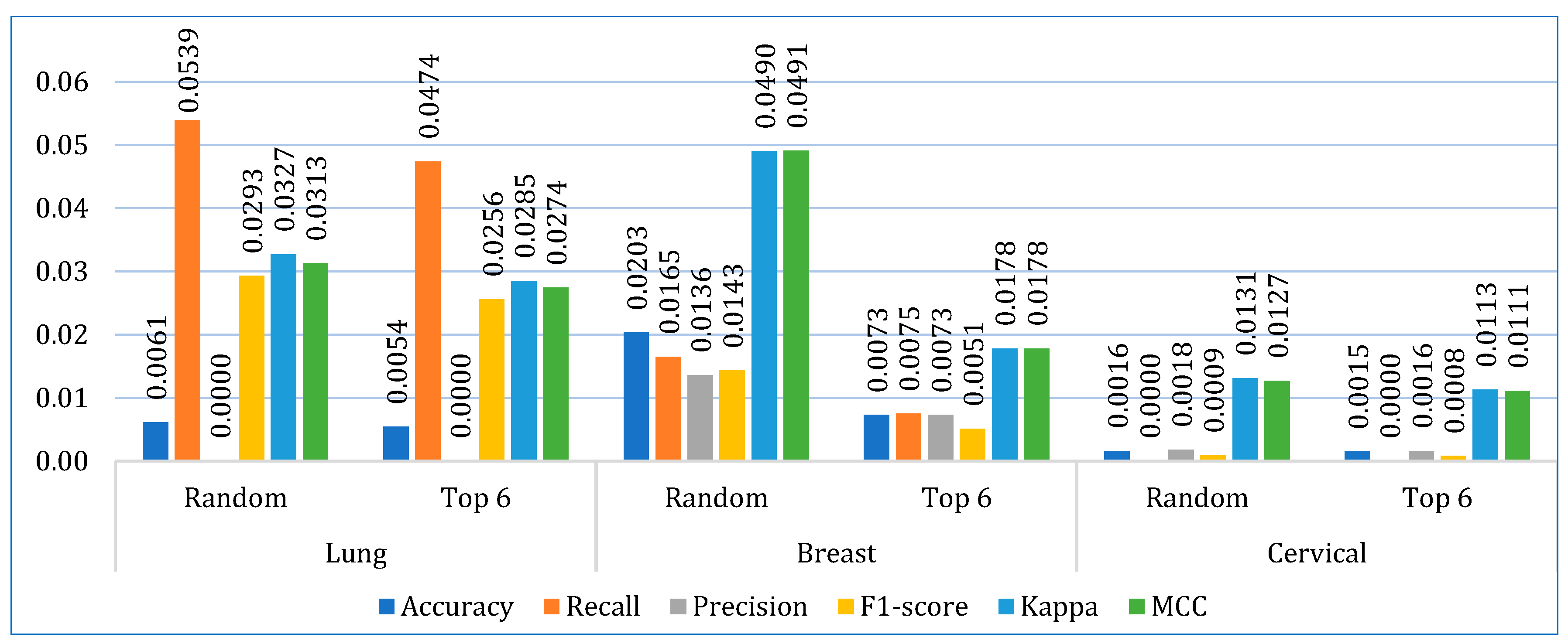
| Dataset | Model | TP | FP | FN | TN |
|---|---|---|---|---|---|
| Lung cancer | Random | 86 | 0 | 2 | 74 |
| Top 6 | 87 | 1 | 0 | 74 | |
| Breast cancer | Random | 96 | 2 | 2 | 111 |
| Top 6 | 94 | 0 | 1 | 116 | |
| Cervical cancer | Random | 210 | 0 | 2 | 236 |
| Top 6 | 214 | 1 | 1 | 232 |
| Reference | Considered Models | Dataset Used | Sample Size | No. of Features | Splitting Ratio (Train:Test) | Highest Accuracy (%) | Recall (%) | Precision (%) | F1-Score (%) | MCC (%) | Kappa | AUC (%) | XAI |
|---|---|---|---|---|---|---|---|---|---|---|---|---|---|
| Abdullah et al. [13] | SVM, KNN, and CNN | Lung cancer dataset UCI machine learning repository | 32 | 56 | - | 95.56 (SVM) | 95.60 | 95.60 | 95.40 | - | - | 95.50 | × |
| Safiyari and Javidan [26] | Bagging, dagging, ADB, MB and random subspace with a combination of several base classifiers | SEER data (released in April 2016) | 643,924 | 149 | - | 88.98 (ADB) | - | - | - | - | - | 94.90 | × |
| Wang et al. [27] | Bagging, RF with BSPL | US National Library of Medicine National Institutes of Health | 720 | 3 | 70:30 | 97.96 (RFSPL) | - | - | 98.11 | - | - | 98.21 | × |
| Siddhartha et al. [28] | Bagging with RF | Wroclaw Thoracic Surgery Centre for Patients (2007 to 2011) | 470 | 17 | 90:10 | 84.04 | 94.28 | 85.71 | 89.79 | - | - | 83 | × |
| Ahmad and Mayya [25] | RF for LCPT | International cancer database and local medical questionnaire | 1000 | 23 | - | 93.33 (RF) | 100 | 81.82 | 90.09 | 93.33 | 84.28 | 100 | × |
| Mamun et al. [29] | XGB, LGBM, bagging, and ADB | Lung cancer dataset by staceyinrobert, Data World | 309 | 16 | 70:30 | 94.42 (XGB) | 94.46 | 95.66 | - | - | - | 98.14 | × |
| Patra [14] | NB, KNN, and RBF | Lung cancer UCI machine learning repository | 32 | 56 | 80:20 | 81.25 (RBF) | 81.30 | 81.30 | 81.30 | - | - | 74.90 | × |
| Zhang et al. [38] | LR, NB, RF, and XGB | UK Biobank | 467,888 | 49 | 70:30 | 98.93 (XGB) | 98.13 | 99.72 | 98.92 | 97.90 | 97.90 | 99.80 | × |
| Radhika et al. [56] | DT, SVM, NB, and LR | Lung cancer UCI machine learning repository (D1) and Data World (D2) | 32 (D1), 1000 (D2) | 57 (D1), 25 (D2) | - | 99.20 (SVM) | 99.01 | 89.99 | 99 | 89.36 | - | 99 | × |
| Jaiswal et al. [30] | SVM, LR, KNN, NB, DT, RF, ADB, XGB, and I-XGB | BCWD | 569 | 30 | 80:20 | 99.84 (I-XGB) | 100 | 99.50 | 98.50 | - | - | - | × |
| Rabiei et al. [31] | RF, GBT, MLP, and GA | Motamed Cancer Institute (ACECR) collected from Tehran, Iran | 5178 | 24 | 75:25 | 80 (RF) | 95 | 84.82 | 89.62 | 78.57 | 78 | 59 | × |
| Nemade and Fegade [20] | NB, LR, SVM, KNN, DT, RF, ADB, and XGB | BCWD | 569 | 30 | 80:20 | 97 (XGB) | 96 | 98 | 97 | - | - | 99 | × |
| Naji and Filali [32] | SVM, RF, LR, DT, and KNN | BCWD | 569 | 30 | 75:25 | 97.20 (SVM) | 94 | 98 | 97.93 | - | - | 96.60 | × |
| Fu et al. [33] | EXSA, Cox, RSF, and GBM | Clinical Research Center for Breast (CRCB) collected from China hospital | 12,119 | 20 | 70:30 | 83.45 (Cox) | - | - | - | - | - | 83.85 | × |
| Uddin et al. [23] | SVM, RF, KNN, DT, NB, LR, ADB, GB, MLP, NCC, and voting | CCrf, UCI machine learning repository | 858 | 36 | 80:20 | 99.16 (voting) | 100 | 100 | 100 | - | - | - | × |
| Alam et al. [34] | BDT, DF, and DJ | CCrf, UCI machine learning repository | 858 | 36 | - | 94.10 (BDT) | 89.60 | 89.60 | 89.60 | - | 86.90 | 97.80 | × |
| Song et al. [35] | LR, DT, SVM, MLP, KNN, and voting | Collected dataset (D1), and CCrf, UCI machine learning repository (D2) | 472 (D1), 858 (D2) | 50 (D1), 36 (D2) | - | 83.16 (voting) | 28.35 | 51.73 | 32.80 | 34.92 | 66.82 | - | × |
| Jahan et al. [36] | MLP, RF, KNN, DT, LR, SVC, GBC and ADB | CCrf, UCI machine learning repository | 858 | 36 | 70:30 | 98.10 (MLP) | 98 | 98 | 98 | 95.22 | 95.22 | 97.61 | × |
| Alsmariy et al. [37] | LR, DT, RF, and voting | CCrf, UCI machine learning repository | 858 | 36 | - | 98.49 (voting) | 98.60 | 95.16 | 98.37 | 58.90 | 72.50 | 99.80 | × |
| Ali et al. [24] | RF, SVM, GNB, DT, and ensemble | Sobar-72 (D1), and CCrf, UCI machine learning repository (D2) | 72 (D1), 858 (D2) | 19 (D1), 36 (D2) | 70:30 | 98.06 (ensemble) | 100 | 98.77 | 98.97 | 98 | 98 | 97 | √ |
| Aravena et al. [39] | XGB, LR, RF, and SVM | Breast cancer patients from Indonesia | 400 | 7 | 75:25 | 85 (XGB) | 85.40 | 79.50 | - | - | - | - | √ |
| Makubhai et al. [40] | DT, LR, RF, and XGB | Five datasets (D1, D2, D3, D4, D5) | 500 (D1), 1000 (D2), 750 (D3), 2000 (D4), 1500 (D5) | 20 (D1), 15 (D2), 25 (D3), 30 (D4), 18 (D5) | 70:30 | 95.5 (XGB) | - | - | - | 91 | 91 | - | √ |
| This paper | LR, NB, KNN, SVM, LDA, CB, GB, XGB, ADB, LGBM, DT, RF, ET, BDT, BME | Lung cancer dataset by staceyinrobert, Data World | 309 | 16 | 70:30 | 99.22 (stacking) | 93.16 | 100 | 96.40 | 96.07 | 95.96 | 98.23 | √ |
| BCWD | 569 | 31 | 98.85 (stacking) | 99.51 | 98.88 | 99.19 | 97.20 | 97.19 | 99.93 | ||||
| Cervical cancer | 835 | 36 | 99.78 (stacking) | 100 | 99.76 | 99.88 | 98.31 | 98.29 | 99.39 |
Disclaimer/Publisher’s Note: The statements, opinions and data contained in all publications are solely those of the individual author(s) and contributor(s) and not of MDPI and/or the editor(s). MDPI and/or the editor(s) disclaim responsibility for any injury to people or property resulting from any ideas, methods, instructions or products referred to in the content. |
© 2025 by the authors. Licensee MDPI, Basel, Switzerland. This article is an open access article distributed under the terms and conditions of the Creative Commons Attribution (CC BY) license (https://creativecommons.org/licenses/by/4.0/).
Share and Cite
Ganie, S.M.; Dutta Pramanik, P.K.; Zhao, Z. Enhanced and Interpretable Prediction of Multiple Cancer Types Using a Stacking Ensemble Approach with SHAP Analysis. Bioengineering 2025, 12, 472. https://doi.org/10.3390/bioengineering12050472
Ganie SM, Dutta Pramanik PK, Zhao Z. Enhanced and Interpretable Prediction of Multiple Cancer Types Using a Stacking Ensemble Approach with SHAP Analysis. Bioengineering. 2025; 12(5):472. https://doi.org/10.3390/bioengineering12050472
Chicago/Turabian StyleGanie, Shahid Mohammad, Pijush Kanti Dutta Pramanik, and Zhongming Zhao. 2025. "Enhanced and Interpretable Prediction of Multiple Cancer Types Using a Stacking Ensemble Approach with SHAP Analysis" Bioengineering 12, no. 5: 472. https://doi.org/10.3390/bioengineering12050472
APA StyleGanie, S. M., Dutta Pramanik, P. K., & Zhao, Z. (2025). Enhanced and Interpretable Prediction of Multiple Cancer Types Using a Stacking Ensemble Approach with SHAP Analysis. Bioengineering, 12(5), 472. https://doi.org/10.3390/bioengineering12050472