Abstract
Macroalgae are an integral part of estuarine primary production; however, their excessive growth may have severe negative impacts on the ecosystem. Although it is generally believed that algal blooms may be caused by a combination of excessive nutrients and temperature, their occurrences are hard to predict, and quantitative monitoring is a logistical challenge which requires the development of reliable and inexpensive techniques. This can be achieved by implementation of processing algorithms and indices on multi-spectral satellite images. Tuggerah Lakes estuary on the Central Coast of NSW was studied because of the regular occurrences of blooms, primarily of green filamentous algae. The detection of algal blooms based on the red-edge effect of the chlorophyll provided consistent results supported by direct observations. The Floating Algae Index (FAI) was identified as the most accurate index for detecting algal blooms in shallow areas, following a comparative analysis of six commonly used algae detection indices. Logistic regression was implemented where FAI was used as a predictor of two clusters, “bloom” and “non-bloom”. FAI was calculated for multi-spectral satellite images based on pixels of 20 × 20 m, covering the entire area of the Tuggerah Lakes. Seven sample points (pixels) were chosen, and the optimal threshold was found for each pixel to assign it to one of the two clusters. The logistic regression model was trained for each pixel; then the optimal parameters for its coefficients and the optimal classification threshold were obtained by cross-validation based on bootstrapping. Probabilities for classifying clusters as either “bloom” or “non-bloom” were predicted with respect to the optimal threshold. The resulting model can be used to estimate probability of macroalgal blooms in coastal estuaries, allowing quantitative monitoring through time and space.
1. Introduction
Macroalgae (multicellular seaweeds) are important contributors to estuarine primary production. They normally grow in estuaries throughout the year, but in warm seasons may significantly increase in biomass, resulting in so-called algal blooms. This is especially common in shallow estuaries throughout the world [1] and can significantly impact the entire ecosystem by inducing hypoxia, smothering seagrasses, and ultimately leading to the loss of estuarine biodiversity [2,3,4,5,6,7]. The optimal temperature for the maximum growth of macroalgae is 25–30 °C [8], which may be a reason why macroalgal blooms occur in seasons when water temperature is within these limits. Low water exchange between an estuary and the sea promotes the accumulation of nutrients which support algal growth in wide areas of shallow warm water [9,10]. Therefore, rapid increase in algal biomass of common opportunistic algae such as Ulva (formerly Enteromorpha) intestinalis, Chaetomorpha linum, and other surface-floating species may serve as an indicator of water eutrophication caused by urban runoff from extensive development of surrounding areas or treated wastewater [11]. Algal blooms can be an indirect indicator of unsustainable agriculture, insufficient wastewater treatment, changes in hydrological processes due to extensive development of the land and human population growth, or any other disturbances of the natural balance of estuaries. Tracking and recording the dynamics of algal growth by remote sensing can be used as an environmental monitoring tool which is suggested for different parts of the world [12,13].
Despite the widespread nature of macroalgal blooms in estuaries throughout the world [1,5], there are very few data on their temporal and spatial dynamics. Monitoring algal blooms at different temporal and spatial scales is the first crucial step in trying to understand the factors that correlate with the presence of the blooms and, ultimately, in developing predictive capabilities for effective management and control of excessive algal growth.
One of the challenges of effective monitoring is developing reliable and inexpensive techniques of measuring algal biomass and/or the area of the blooms. Substantial efforts have been made into the development of measurement techniques that would allow effective monitoring of blooms at large scales in multiple estuaries [14,15]. As direct measurements in the field are impractical, especially at very large scales, remote sensing is the most promising tool for quantifying and mapping the distribution and abundance of floating macroalgae.
In ecological studies, the use of satellite images is an effective non-invasive method of observation allowing monitoring at large spatial scales. Analysis of multi-spectral data enables the detection of areas with certain reflection patterns or spectral signatures. Detection of algal blooms using the spectral signatures of pigments was suggested after this approach was successfully implemented for biomass measurements of terrestrial vegetation [16,17]. The detection of algal mass by remote sensing is literally the detection of the light reflection patterns of individual pigments common in the algae [18,19].
The biological role of photosynthetic pigments is absorbing light energy and then transferring it to photosynthetic reaction organelles or re-emitting excessive energy at longer wavelengths to prevent photodamage of the cell. The distinctive feature of all types of chlorophyll is fluorescence in the near infra-red diapason, when the lowest reflectance in the range of 630–650 nm changes to the highest in the near infra-red of 685 ± 25 nm [20,21,22]. This produces the so-called “red-edge” effect, which is used as a specific optical feature in chlorophyll detection [23,24].
Analyses of satellite images based on the “red-edge” effect have been widely used to estimate chlorophyll activity in terrestrial plants [16,18] and for detecting algal blooms in large areas such as the Yellow Sea [25,26,27,28,29]. Theoretically, submerged vegetation may exhibit spectral characteristics similar to those of algal blooms. However, water absorbs radiation in the near-infrared (NIR) range exponentially, and at depths greater than approximately 5 cm, the signal-to-noise ratio becomes too low to reliably detect chlorophyll using NIR-based indices [30]. This approach enables a clear distinction between floating macroalgae on the surface and the water body itself, even in the presence of benthic vegetation such as seagrasses [31].
Initially, only massive bloom events could be detected using images obtained from Moderate Resolution Imaging Spectroradiometers (MODIS) on board the Terra and Aqua satellites due to their 500 m resolution [32]. However, with recent enhancements of satellite sensors, more detailed images could be obtained, which allowed monitoring smaller areas [33]. The spatial distribution of aquatic vegetation in remote sensing data is commonly identified through raster algebra—processing raw satellite imagery using index-based formulas. In some cases, such as distinguishing between different groups of photosynthetic organisms (e.g., floating vegetation, submerged aquatic vegetation, and microalgae), multiple indices are applied in combination [31,34]. Additionally, these indices can be used to quantify harvestable accumulations of macroalgal biomass [35].
Machine learning algorithms for pixel-based classification of hyperspectral imagery have already been successfully employed to identify patches of various algal species [36].
The success of machine learning applications for the detection and prediction of algal blooms depends heavily on the selection and preprocessing of input data [37]. Effective model training requires a sufficiently large dataset that incorporates environmental and hydrological variables. Existing models known to the authors have determined the presence or absence of macroalgal blooms based on cell concentrations in water samples or chlorophyll activity [13,38].
Mathematical models have proved to be a reliable tool in studies of species dynamics (such as phytoplankton, algae, and other water-dependent organisms) in connection with environmental conditions such as water salinity or toxins release during harmful algae blooms [39]. A fractional regression model was implemented in a study of rural production performance [40]. Modeling proved to be effective in the reduction of harvest operations costs [41]. In our study, the results were obtained by the development of a model based on a logistic regression algorithm and training it on sample point data.
Overview of Existing Indices
Satellite images are currently available as top-of-atmosphere radiances (level 1 data) and atmospherically corrected surface-leaving radiances (level 2 data) [42]. For calculations of any surface phenomena, like the spectral signature of the algae, which is basically the light reflected from their surface, it is preferable to have level 2 data, where algorithms for atmospheric effects correction are implemented and unwanted effects are minimized [22,43]. All known indices are based on an FLH (Fluorescence Line Height) algorithm, which calculates the difference between reflection in 685 ± 25 nm (near infra-red, NIR) and in shorter (red) and in longer (infra-red) reflections. However, some of them introduced reflectance in the green and blue bands to increase the capability of the algorithm to distinguish the spectral signature of the floating macroalgae from the surrounding water.
The first index developed for terrestrial vegetation monitoring is TVI (Transformed Vegetation Index). It was designed to be used with bands 5 and 7 of the satellite ERTS-1 (Earth Resources Technology Satellite-1) MSS (Multi-Spectral Scanner), or Landsat-1. The MSS recorded data in four spectral bands: green, red, and two infrared bands.
where the Band Ratio Parameter (BRP) is calculated as follows:
where:
R(NIR)—reflection in the near infra-red diapason, which is Band 7, and
R(RED)—reflection in the red diapason, Band 5.
The Band Ratio Parameter (BRP) was initially introduced as a component of the TVI by Rouse et al. [16]. In subsequent studies, this component was used independently and became known as the Normalized Difference Vegetation Index (NDVI), although the mathematical formula remains the same. The key distinction lies in their application: BRP is embedded within the TVI framework, whereas NDVI is widely applied as a standalone index. The difference between reflection in the red and near infra-red diapasons proved to be a reliable basis for the development of future indices.
The NDVI (Normalized Difference Vegetation Index) is calculated in the same manner as BRP. It is currently used for the detection of chlorophyll concentration in terrestrial plants [44]:
where:
R(NIR)—reflection in the near infra-red diapason, and
R(RED)—reflection in the red diapason
Currently, the NDVI is a basic raster analysis tool for estimating the condition of terrestrial vegetation. However, it has limited use for aquatic flora because the sensor is unable to obtain reflectance in the near infra-red diapason from submerged vegetation.
The FAI (Floating Algae Index) was developed for the detection and mapping of massive algal blooms on the sea surface. It shows chlorophyll activity and was first implemented on medium-resolution (250–500 m) MODIS images. FAI detects organisms with a red-edge effect of plant tissue above the water, allowing separation of macroalgae from phytoplankton suspended in the water column [25]. This index shows the relative height of the near infra-red peak relative to the background value, which is interpolated from the surrounding red and short-wave infrared (SWIR) wavelength values:
where:
R(RED) is the Rayleigh-corrected top of atmosphere reflection in the red diapason,
R(NIR)—Rayleigh-corrected top of atmosphere reflection in the near infra-red diapason,
R(SWIR)—Rayleigh-corrected top of atmosphere reflection in the short-wave infra-red diapason,
λ(RED)—median wavelength in the red diapason,
λ(NIR)—median wavelength in the near infra-red diapason and
λ(SWIR)—median wavelength in the short-wave infra-red diapason.
Importantly, FAI is sensitive to water turbidity as it also reflects infra-red radiation and therefore can give false positive results [45,46].
The NDAI (Normalized Difference Algae Index) uses the same scheme as NDVI that is based on the difference between the reflectance in the red and NIR diapasons. Technically, it is the NDVI index applied to atmospherically corrected data. The correction is based on the images taken in the SWIR diapason.
where: —top of atmosphere reflectance in the near infra-red diapason,
—atmospheric correction for the near infra-red diapason,
—top of atmosphere reflectance in the red diapason, and
—atmospheric correction for the red diapason.
The index has large negative results for clean blue ocean waters, which have low reflectance in both the red and NIR diapasons. In turbid conditions, suspended inorganic particles in the water column cause higher reflectance in the red diapason and lower reflectance in the NIR diapason. In this case, NDAI may show low positive or slightly negative values (i.e., indicating the presence of algae when there is none). Algae have low reflectance in the red diapason and high in the NIR diapason, so the index will have high positive values when a macroalgal bloom is present [47].
The SAI (Scaled Algae Index) is an algorithm used to calculate the spatial extent of floating algae [46]. Its implementation requires several steps. First, the index, which detects chlorophyll (NDVI or FAI), is calculated. Then an odd-numbered square pixel is selected around each pixel, and the median value calculated for this region and applied to the central pixel. A new raster is filled with these values. The resulting raster has the same configuration and number of pixels but a smoothed picture with high variability of an image removed. Then, the empirically selected threshold is applied, and all pixels are divided into “algae” and “non-algae” categories. This approach works well on large areas of the Yellow Sea. However, the number of pixels on the side of the square region which is used to extract the median value needs to be smaller than the number of pixels across the entire area of the bloom, otherwise the high index values may be replaced with the lower median value, and some data will be lost. For smaller lakes, the application of the median value can be skipped, and the threshold can be applied directly to the index raster. The resulting number of “bloom” pixels is used to calculate the area of the bloom. At the last step, the area of the bloom is calculated as a product of the number of pixels showing a positive result (“bloom” pixels) multiplied by the area depicted by one pixel (spatial resolution of a sensor). This index also considers the value of the “bloom” pixel and calculates the relative algae coverage in the area covered by this pixel.
The SABI (Surface Algal Bloom Index) is an empirical algorithm developed for processing MODIS images [27]. It is targeted to estimate the area of floating macroalgae. It uses the “red-edge effect” in the numerator and incorporates blue and green bands in the denominator, which is supposed to make it less dependent on atmospheric effects and Rayleigh scattering. SABI is calculated as follows:
where:
R(NIR)—reflection in the NIR diapason,
R(RED)—reflection in the red diapason,
R(GREEN)—reflection in the green diapason, and
R(BLUE)—reflection in the blue diapason.
SABI can be implemented on Sentinel 2 data and was considered in further analysis.
The MERIS MCI (Medium Resolution Imaging Spectrometer—Maximum Chlorophyll Index) proved to be effective for detecting cyanobacteria blooms in turbid eutrophic waters where suspended matter increase reflection in the visible diapason and can mask the chlorophyll spectral signature. It also detects surface blooms of microalgal films or floating macroalgal mats. However, for macroalgae, its application is limited because of high chlorophyll content in their floating biomass, which may be compared to those in plants. In this case MCI may show “out-of-range” (too high) results, as for terrestrial vegetation [48]
Based on MERIS data, MCI calculates the height of the peak in reflection at 709 nm against a baseline formed by reflections at 681 and 753 nm. But it is versatile and can be adopted for other satellite sensor bands with different wavelengths.
where:
R—atmospherically corrected water-leaving reflection
681, 709, and 753—central wavelengths of bands used in calculation.
The VB-FAH (Virtual Baseline Floating macroAlgae Height) algorithm was developed for mapping macroalgal blooms in the Yellow Sea and proved to be insensitive to atmospheric effects and solar/viewing position [28]. It is a peak-above-baseline method which uses the difference between an artificial baseline and the height of the reflectance peak in NIR. The difference from the previously described MERIS MCI is that the baseline is formed by reflections in the red and green diapasons, which, in the case of floating algal mats, have smaller values than reflectance in NIR:
where:
R(GREEN)—reflection in the green diapason,
R(RED)—reflection in the red diapason,
R(NIR)—reflection in the near infra-red diapason,
λ(GREEN)—median wavelength in the near infra-red diapason,
λ(RED)—median wavelength in the red diapason,
λ(NIR)—median wavelength in the near infra-red diapason.
As this index was developed to be used with Sentinel 2 images to pick up macroalgae mats, it was selected for our analysis too.
The FGTI (Floating Green Tide Index) approach is based on the enhancement of raw digital data using a matrix of coefficients developed for each sensor. This increases the difference between clear water and floating algal mats. This method allows the use of images without atmospheric correction and can detect macroalgae through thin cloud coverage and has been successfully used for monitoring floating Ulva prolifera mats in the Yellow Sea [15]. Because this approach does not include any map algebra to select bloom areas and appears to be sensor-dependent (coefficients are unique for each sensor), we did not use it further.
The ABDI (Algal Bloom Detection Index) was developed for use with Sentinel 2 Bands [33]:
where:
R(GREEN)—reflection in the green diapason (545–575 nm),
R(RED1)—reflection in the red diapason (645–665 nm),
R(RED2)—reflection in the red-edge 2 diapason (740 nm),
R(NIR)—reflection in the near infra-red diapason (859–865 nm),
λ(RED1)—median wavelength in the red diapason used (645–665 nm),
λ(RED2)—median wavelength in the near infra-red diapason, and
λ(NIR)—median wavelength in the narrow near infra-red diapason.
ABDI takes advantage of extended red-edge bands as Sentinel 2 provides three diapasons for plant red-edge effect detection. It also uses the green band where chlorophyll has the strongest reflection.
Indices whose formulae incorporate the median wavelength of the spectral bands used (ABDI, FAI, MCI, VB-FAH) can be applied to data from different sensors, as variations in wavelength are accounted for in the coefficients (MODIS, Landsat, Sentinel) [49].
The primary aim of this study was to assess and identify the most reliable among the known indices for the detection of macroalgal blooms. To allow the analysis to be used at different sun angles and light intensity, the index should be ratio-dependent [50].
A secondary aim was to develop effective techniques for identifying and quantifying macroalgal blooms, facilitating efficient monitoring and measurement of their abundances.
The study outlines the selection of the most suitable index for detecting algal blooms, applied to multispectral imagery of the lake surface. The output of the index is then used to develop a model based on logistic regression. The paper also discusses the challenges associated with classifying index values in cases where submerged aquatic vegetation is present near the water surface.
2. Methods
2.1. Selection of “Candidates” for the Optimal Index
For the selection of the best index for macroalgae bloom detection, the Web of Science and Scopus databases were searched following the methodology of Lyons et al. [5]. The focus of the search was algorithms for the interpretation of remote sensing data for chlorophyll spectral signature detection.
The search terms for multi-spectral satellite images interpretation and keywords for chlorophyll activity were combined using the Boolean operator “AND”. The keywords for chlorophyll reflectance and algal blooms were separated by the operator “OR” and then combined into a search string. The following search terms for remote sensing and multi-spectral data processing were used:
| Remote Sensing and Multi-Spectral Data Processing | AND Algorithms and Indices | AND Macroalgal Blooms |
| “Satellite Remote Sensing” OR “Remote sensing” OR “Multi spectral” OR “Chlorophyll Index” OR “Spectral signature” OR “Chlorophyll fluorescence” OR “Vegetation monitoring” OR “Water leaving radiance” OR “Reflectance” OR “Red edge effect” OR “MODIS” OR “ERTS” OR “MERIS” OR “Sentinel” OR “Bloom monitoring” | “ABDI” OR “Algal Bloom Detection Index” OR “FAI” OR “Floating Algae Index” OR “FGTI” OR “Floating Green Tide Index” OR “MCI” OR “Maximum Chlorophyll Index” OR “NDAI” OR “Normalized Difference Algae Index” OR “NDVI” OR “Normalized Difference Vegetation Index” OR “SABI” OR “Surface Algal Bloom Index” OR “SAI” OR “Scaled Algae Index” OR “TVI” OR “Transformed Vegetation Index” OR “VB-FAH” OR “Virtual Baseline Floating macroAlgae Height” OR “FLH” OR “Fluorescence Line Height” OR “Spectral Index” OR “Chlorophyll Index” | “Macroalgae” OR “Macroalgal Blooms” OR “Floating vegetation” OR “Chlorophyll content” OR “Green macroalgae” OR “Floating macroalgae” OR “Ulva” OR “Enteromorpha” OR “Chaetomorpha” |
Information about existing indices that can be used for macroalgal bloom detection was collected. After reviewing the ten indices listed above, four were excluded from further consideration. TVI was removed because it was developed for different spectral ranges and is essentially a predecessor of NDVI. NDAI was excluded because it was designed to work with atmospheric correction, while the data available in this study have already been corrected, and no further correction was necessary. SAI is an algorithm for estimating the surface area of floating algae based on a chlorophyll activity index, such as FAI. FGTI appears to be sensor-specific and not transferable. Therefore, six indices were selected for further comparison: NDVI (Normalized Difference Vegetation Index), SABI (Surface Algal Bloom Index), FAI (Floating Algae Index), ABDI (Algal Bloom Detection Index), MCI (Maximum Chlorophyll Index), and VB-FAH (Virtual Baseline Floating macroAlgae Height). These six indices were applied to a fragment of a satellite image of the coastal zone of Tuggerah Lakes (ground truth area at Chittaway Bay), and the resulting rasters were compared with field observations and drone imagery. An index performance analysis was then conducted, and the accuracy of each index was calculated. The index with the highest accuracy was selected for further study.
For quantitative validation of our interpretation of the satellite data, aerial photos were taken by a drone (DJI Phantom 4 Pro V2.0, camera DJI FC6310S) flying over the Chittaway Bay area of Tuggerah Lakes at a height of approximately 30 m. The images were georeferenced, the contours of algal bloom mats digitized, and the area measured using ESRI ArcGIS 10.7 software. Simultaneous capture of satellite images and drone photos involved using satellite images from the same date as the drone imagery. Bloom data obtained by index implementation on multi-spectral satellite images were compared with drone photos and the results of the direct observation were used to select the best-performing index formula. Performance of the index was defined as the best correspondence with the macroalgal mats contours, digitized from drone photos. The efficiency of each index was calculated as the ratio of the sum of true positives and true negatives to the total sum of pixels. It was applied to multi-spectral satellite data spanning from 2019 to 2023, involving the processing of a total of 170 images.
2.2. Study Area
The initial study of algal blooms and verification of data on the ground was carried out on the Tuggerah Lakes on the Central Coast, New South Wales, located 70 km north of Sydney. The Tuggerah Lakes system consists of three interconnected lakes that form a saline barrier estuary of approximately 80 km2 area and an average depth of 2.4 m. This area is characterized by a temperate oceanic climate, with warm summers and mild winters. The average summer air temperature is approximately 25 °C, while the winter temperature averages around 11 °C. The water temperature in the lakes also varies seasonally, reaching its peak in February and March at approximately 23 °C. The lowest average water temperatures, around 18.6 °C, are typically recorded between May and August. The estuary experiences regular macroalgal blooms [51,52], which makes it optimal for satellite, drone, and on-ground observations.
Sample points on the lake were selected in areas where the conditions for algal blooms were optimal: shallow depth, good light exposure, and weak currents (Figure 1, for precise coordinates of the sample points see Table 1). Other features of those places which can affect the index results (seagrasses presence, shallow or turbid water) were also considered when selecting control points. Having these obstacles was important for selecting the most accurate threshold. For comparison, points where no bloom occurred were also chosen, but they were subsequently discarded during further processing as they were deemed unnecessary for training of the model.
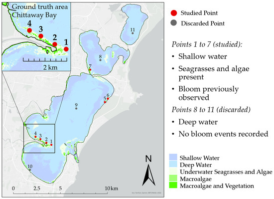
Figure 1.
Sample points for algorithm training selected in the Tuggerah Lakes estuary.

Table 1.
Coordinates of sample points on Tuggerah Lakes (WGS_1984_UTM_Zone_56S).
A smaller area of Chittaway Bay was selected for ground truthing because of the diversity of seagrasses and algae and repeatedly observed blooms.
2.3. Logistic Regression Model
The model operates on preprocessed Sentinel-2 MSI. The primary reason for choosing these data is higher spatial resolution compared to MODIS (20 m vs. 500 m), which is critically important for studying estuaries—relatively small and spatially complex environments—especially when considering the even smaller areas affected by algal blooms. For accurate detection, the target size (in this case, the extent of the algal mat) must exceed the sensor’s spatial resolution by at least twice [30].
Eleven training datasets were used, each of which had 166 records or timesteps collected over 4 years (dates 1 January 2019 to 18 February 2023). For all timesteps for each of the eleven dataset points, “bloom”/“non-bloom” status was established. This status was used along with the date when an image was taken to train the model to detect the probability of the bloom using logistic regression. The timesteps for these records were irregular due to varying cloud cover, which completely obstructed aerial visibility on some days. As an algorithm of algae bloom detection, single variable logistic regression was used. As logistic regression is a basic method for classification of values into two clusters, it was used for model development. Analytically, this model is given by the equation:
The variable x is an index value, and p(x) is an output, which is interpreted as a probability of a bloom presence. For each pixel in the model, the value of p(x) (1) was estimated using the maximum likelihood method. Then, the estimated values and were used for determining the probability .
The probability threshold was established based on index values for binary (“bloom”/“non-bloom”) classification, quantified as 0 and 1, respectively. For this estimation, the Python 3.13.3 language was utilized. After implementation of a bootstrapping technique, the optimal threshold was found for each of the points. Cross-validation based on bootstrapping of the prediction function was performed to classify “bloom”/“non-bloom” events with respect to the optimal threshold. The cross-validation procedure is described below.
The algorithm was as follows: the given pixel was classified as a “bloom” if the estimated value exceeded some threshold po, and “non-bloom” otherwise. Therefore, the blooming prediction algorithms were established for each pixel (sample point) using three parameters, , , and po. Optimal thresholds po were identified by minimizing the classification error: the percentage of wrongly classified pixel values.
For index implementation, we used Sentinel 2 multi-spectral images taken between 2019 and 2023.
The results show overlap values attributed to “bloom” and “non-bloom” because of the similarity of the spectral characteristics of floating algae and seagrasses in the shallow water.
Therefore, this represents an example of a binary classification, and the most logical approach to solve it is logistic regression (Figure 2).
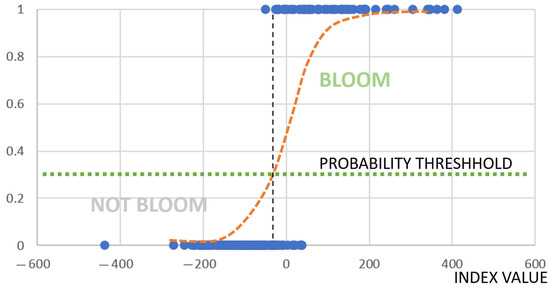
Figure 2.
Stylized diagram illustrating how logistic regression works. Blue points represent the observed values of the Boolean variable predicted by logistic regression (0 = non-bloom, 1 = bloom). The estimated logistic regression curve is shown as a red dashed line. The vertical dashed line marks the critical index value that separates predicted blooms from non-blooms. This line intersects the logistic curve at the same point where the horizontal dotted line—representing the probability threshold—crosses it.
During training and calibration of the model, logistic coefficients which define the curve and probability threshold were calculated.
3. Results
3.1. Selection of the Optimal Index
For floating macroalgae, having a water surface as a background initially seems to simplify the task. However, coastal shallow zones vary greatly in terms of vegetation composition and type, and not all of it can be attributed to macroalgal blooms. Seagrasses also photosynthesize, but usually they do not constitute a problem unless found in very shallow water. For example, in the RGB image (Figure 3), only the top two fragments can be attributed to blooming, while the others should be classified as non-blooming, despite the visual similarity between fragments of the image taken on underwater seagrasses and the actual algal bloom. This was the challenge of the classification task—when the spectral composition at certain points could be classified as both “bloom”/“non-bloom”. The outstanding spectral characteristic of the algal mat is high chlorophyll activity, producing a red-edge effect. Therefore, the challenge was to find the threshold index value by which it would be possible to detect “bloom” pixels attributed to the algal bloom.
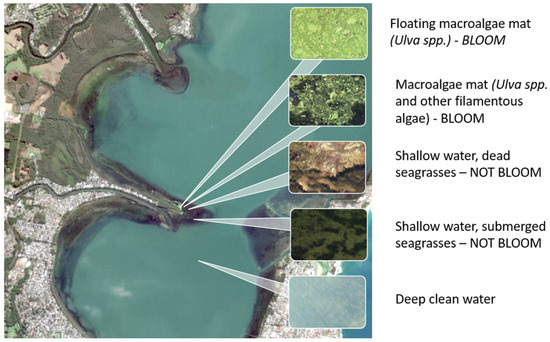
Figure 3.
RGB image of study area showing similarities in bloom and non-bloom areas.
The following procedure was developed to select the index that best distinguished coastal algal blooms occurring in shallow turbid water where seagrasses may also be present. A study area was chosen using drone footage which was captured simultaneously with a satellite image. Six indices were applied to the same multi-spectral image of the ground truth area. Out of the six studied indices, two (NDVI and SABI) already had binary values, indicating pixels where chlorophyll activity is present or absent.
Four non-binary rasters (FAI, VB-FAH, MCI, and ABDI) were reclassified using the Slice tool from ArcGIS Map Algebra to standardize them for subsequent comparison. The Natural Breaks method was applied for greater contrast. Following classification by the Slice method for all indices, a uniform threshold of 100 was established based on statistics calculated by ArcGIS tools supported by visual assessment, categorizing pixel values as either “bloom” (chlorophyll is present) or “non-bloom” (chlorophyl is absent).
Therefore, six binary “bloom”/“non-bloom” rasters were obtained. The next step involved comparing these binary rasters with the results from the drone photo processing. Digitized contours of algal mats from the drone photo were overlaid onto the raster of the satellite image (Figure 3). Algal blooms could be easily identified from the drone images and, thus, pixels within detected algae mats were selected to determine true positive and negative, as well as false positive and negative pixels. Grid corresponding with Sentinel-2 MSI pixels (20 × 20 m resolution) was applied on the algal mats contours, and pixels affected by bloom marked green (Figure 4).
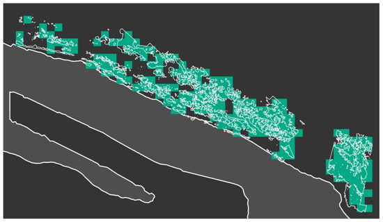
Figure 4.
Digitized algae mats obtained by the drone photo over the satellite image pixels.
Figure 5 presents a comparison of the results obtained from application of six selected indices on MSI of ground-truth area with the digitized algae mats, as derived from drone imagery shown in Figure 4.
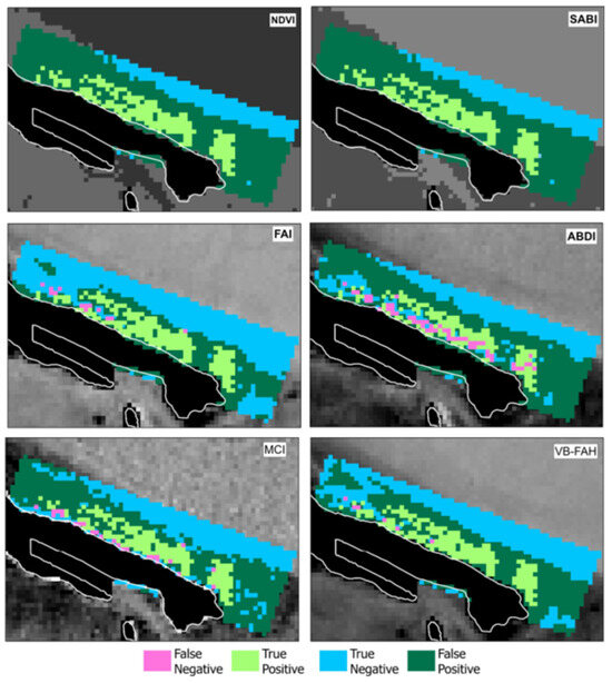
Figure 5.
Indices performance comparison.
NDVI proves effective for identifying floating algal mats, as the spectral characteristics of macroalgae above the water surface are similar to those of terrestrial vegetation. The index also yielded positive results in shallow nearshore areas, suggesting that it detects submerged seagrasses as well. A similar outcome was observed for SABI. For all indices, the number of correctly and incorrectly identified pixels was calculated, which served as the basis for assessing the accuracy of each index.
Some difference in the total number of pixels for VB-FAH and MCI can be attributed to variations in the formulas for index calculation and the ranges involved.
To assess how accurately each index identifies true positive and negative values (i.e., “bloom”/“non-bloom”), the following equation was used:
where:
IA is the index of accuracy (a larger value indicates better performance),
TP is the number of true positive pixels,
TN is the number of true negative pixels,
TPxls is the total number of pixels in the studied fragment of the satellite image with the index implemented.
When applied to Sentinel-2 imagery, FAI demonstrated high precision when compared with detailed aerial photographs—showing noticeably fewer false positives.
Figure 6 presents a comparative analysis of the effectiveness of various indices applied to the same area. The bottom part of the diagram shows the number of correctly identified pixels, whose values match the results of direct observation. Notably, the algorithms FAI, MCI, ABDI, NDVI, and SABI each yielded 978 pixels, whereas MCI resulted in 954 pixels, and VB-FAH yielded 949 pixels. This discrepancy can be attributed to the specific way data are processed by the MapAlgebra tool. However, since accuracy is calculated as the ratio of correctly identified pixels to the total number of pixels, this minor variation has no noticeable impact on the overall accuracy value. As observed in Figure 6, FAI demonstrated the highest efficiency and was therefore selected for further analysis and modeling.
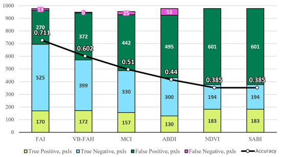
Figure 6.
Pixel count and indices performance analysis.
As a result, several factors contributed to the decision to select FAI for further study:
- High Classification Accuracy: Among the evaluated indices, FAI demonstrated the highest accuracy in distinguishing between “bloom” and “non-bloom” pixels when compared with ground-truth data derived from drone imagery. This was confirmed through pixel-based performance evaluation, where FAI yielded the highest number of correctly classified pixels.
- Sensitivity to Surface-Floating Algae: FAI was specifically designed to detect chlorophyll-rich surface features using the red-edge effect, making it well suited for identifying floating macroalgae. FAI effectively captures the spectral signature of floating mats rather than submerged vegetation or suspended phytoplankton.
- Compatibility with Sentinel-2 Data: The index can be accurately implemented using Sentinel-2 MSI imagery, which offers relatively high spatial resolution (20 m)—a critical factor for detecting comparatively small and spatially complex bloom areas in estuarine environments. FAI’s reliance on red, NIR, and SWIR bands aligns well with Sentinel-2’s spectral capabilities.
- Robustness in Shallow, Turbid Waters: In comparison to indices like NDVI or MCI, which may be confounded by bottom reflectance or suspended sediment, FAI provided more consistent results in shallow and optically complex areas of Tuggerah Lakes.
- Transferability and Simplicity: FAI’s mathematical formulation is relatively simple and does not rely on sensor-specific calibration, making it suitable for application across different satellite platforms and study sites. This makes it a scalable option for future estuarine monitoring efforts.
Together, these factors justify the selection of FAI as the most operationally effective index for macroalgal bloom detection in this study.
3.2. Model Training and Cross-Validation
Seven pixels for which the information about blooming/non-blooming was recorded for 166 consequential days were selected as calibration data (Figure 1). However, the time periods between these days were not constant, as satellite photos were taken at irregular time steps because of the meteorological conditions and characteristics of the satellite orbit. For each of these images, the grid-code, or FAI value was recorded. So, the calibration data were constituted from the seven datasets (for points 1 to 7, Figure 1), each of which had input (FAI value) and output (binary code 0 for non-blooming and 1 for blooming). For the model calibration, the FAI values for each pixel were normalized:
where x is an original FAI value at the sample point, is the sampling mean, and s is the sampling standard deviation. Then, the logistic regression model was run on the normalized data along with a naïve (basic) classification, where positive values were attributed to bloom and negative to non-bloom states.
The sensitivity of a model (TP/(TP + FN) assesses the model’s ability to identify all positive instances correctly. It calculates the proportion of true positives out of all instances that constitute an algal bloom (true positives plus false negatives). Sensitivity analysis provides insights into the model’s ability to capture all occurrences of algae bloom. A high sensitivity value indicates a low number of false negatives.
To assess the practicability of the model, its results were compared with the naïve classification. As can be seen from Table 2 and Table 3, logistic regression gives a lower overall error rate.
Table 2.
Confusion matrix for naïve classification.
Table 3.
Confusion matrix for the optimal basic logistic regression.
Three model parameters—overall error rate, and the quantity of false negatives and false positives—were selected for the model training (calibration). As the values of these parameters could lead to model overestimation, or artificial deflation of the calibration error, a cross-validation test was implemented to select the model coefficients which minimize the test error.
As a result of calibration, the logistic coefficients and were estimated for each of seven pixels (Table 4). An error minimization procedure was implemented for selecting the optimal value of the probability threshold po which corresponded to the maximum accuracy of the model. For each pixel threshold, po was changed from 0.1 to 0.9 with a step of 0.1. Then, the bootstrap resampling procedure was implemented 100 times for each value of the probability threshold. For each value of the threshold, the mean accuracy was calculated. Accuracy is defined in this algorithm as a complement of the overall classification error: Acc = 1 − Err, where the classification error Err is a percentage of the wrongly classified values (sum of false positive and false negative divided by the total number of observations).
Table 4.
Logistic coefficients and and probability threshold po for seven sample points (optimal basic logistic regression).
Logistic regression estimates were implemented for each of these 100 samples, resulting in 100 estimates for and . Once the 100 bootstrap iterations were completed, the mean accuracy was calculated. The bootstrapping method utilizing resampling with returnings was used in the present study. A detailed description of this method, as well as the program codes utilized, can be found in James et al. [53]. The optimal threshold for each sample point was selected as the one delivering the maximum value of the mean accuracy across all iterations (Table 5 and Table 6).
Table 5.
Confusion matrix for bootstrapped results.
Table 6.
Logistic coefficients and and probability threshold po for seven sample points—bootstrapped results.
Figure 7 demonstrates the error rate with respect to the threshold values for the first of 100 bootstrap iterations implemented for the sample point 1 and sample point 4. One iteration was selected to make the graphical illustration clearer. For these figures, the blooming error means the percentage of “bloom” classified as “non-bloom” (percentage of false negative results) and the non-blooming error is the percentage of non-blooms classified as blooms (percentage of false positives).
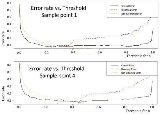
Figure 7.
Error rate as a function of threshold for sample points 1 and 4, for 100 bootstrap iterations.
To evaluate the effectiveness of the modeling approach, error rates were compared among the naïve forecast, optimal logistic regression, and bootstrap test. As shown in Table 2, Table 3 and Table 5, the overall error rates for the naïve forecast were consistently higher than those for the optimal logistic regression model and bootstrapping, with the latter two exhibiting similar performance. Figure 8 presents the total classification errors for all three models, where the solid line, representing the logistic regression model, remains consistently below the dashed line, which corresponds to the naïve forecast. The bootstrapping results (dotted line) closely align with those of logistic regression, exceeding them by no more than 0.02% at sample point 1 and no more than 0.1% at the remaining six sample points. These findings indicate that the model successfully passed the bootstrapping test.
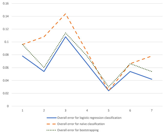
Figure 8.
Error rate for different classification at sample points 1 to 7.
4. Discussion
This study presents two key contributions to the remote detection of macroalgal blooms in estuarine systems. First, it introduces a systematic methodology for selecting the most suitable satellite-derived index to detect blooms using Sentinel-2 multispectral imagery. Second, it applies a logistic regression model to determine an optimal probability threshold for classifying pixels as “bloom” or “non-bloom” based on the selected index.
The primary contribution lies in the index selection process. A literature review following the methodology of Lyons et al. [5] was conducted using the Web of Science and Scopus databases to identify spectral indices relevant to chlorophyll detection in shallow and turbid waters. The focus was on indices compatible with Sentinel-2 data and capable of reliably identifying floating macroalgae. Six candidate indices were selected for evaluation.
These indices were applied to a multispectral image of the Tuggerah Lakes estuary, an area known to experience macroalgal blooms. Using an arbitrary threshold, each index was used to classify pixels as either “bloom” or “non-bloom.” Since ground-truth data on bloom conditions were available for the image, a supervised classification framework was used, enabling the calculation of confusion matrices and accuracy scores for each index. The Floating Algae Index (FAI) achieved the highest classification accuracy (0.711) and was thus selected for further analysis.
This finding is consistent with previous studies that have demonstrated the effectiveness of FAI in detecting floating vegetation, including algal blooms. For example, Hu [25] showed that FAI outperformed traditional NDVI-based approaches in isolating surface-floating algae from water backgrounds, particularly under varying atmospheric conditions. Similarly, Kutser [54] highlighted the limitations of single-band or simple ratio indices in optically complex waters, suggesting the need for more specialized indices like FAI when working in estuarine or coastal systems.
The second component of the study involved calibrating a logistic regression model to establish an optimal probability threshold for classifying bloom presence based on FAI values. The model was trained and validated using data from seven pixels with confirmed bloom activity during the observation period. Bootstrapping was employed to estimate the regression coefficients and assess model stability. While the model cannot be used to predict future bloom events—since FAI values must be calculated from existing imagery—it offers a practical tool for detecting blooms in regions where on-site observation is not feasible, provided suitable satellite data are available.
Comparable approaches have been explored in other studies using statistical classification or machine learning models for bloom detection. For instance, Huang et al. [55] used linear discriminant analysis for classifying cyanobacterial blooms, while Yun [56] applied logistic regression to predict bloom probability using MODIS-derived indices. Our study contributes to this growing body of research by demonstrating that even relatively simple models, when combined with a carefully selected index like FAI, can provide reliable classification in shallow, estuarine environments.
The methodology developed here can support ongoing monitoring efforts in estuarine and coastal environments. The FAI-based classification, when applied to high-quality satellite imagery, effectively identifies algal mats and enables spatially explicit assessments of bloom extent. As remote sensing technology advances and new sensors with higher spectral and spatial resolution become available, the potential to differentiate algal species through spectral signatures may further enhance detection capabilities. For example, previous research on phytoplankton blooms suggests that the use of hyperspectral data could enable more refined classification of bloom species [57,58,59].
Future research should focus on expanding the logistic regression model to incorporate additional environmental variables, such as water temperature, nutrient levels, and seasonal factors. Incorporating lagged or time-series variables through dynamic regression approaches could substantially improve the model’s predictive capacity. Integrating satellite-derived indices with hydrological and meteorological data will ultimately enable the development of early warning systems for algal blooms, supporting more timely and targeted management responses.
5. Conclusions
This study demonstrates that the combination of multispectral satellite imagery with spectral index-based classification and logistic regression modeling provides a reliable, low-cost approach to detecting macroalgal blooms in estuarine environments. Through comparative analysis of six widely used spectral indices, the Floating Algae Index (FAI) was identified as the most accurate for detecting surface-floating macroalgae in the optically complex waters of Tuggerah Lakes. The logistic regression model, calibrated using FAI values and validated through bootstrapping, proved effective in classifying bloom and non-bloom states with high accuracy and low classification error.
While the model is not predictive in a temporal sense—since it relies on contemporaneous imagery—it offers a practical tool for spatially explicit bloom detection where in situ monitoring is not feasible. These results lay the groundwork for further development of predictive frameworks that integrate remote sensing data with environmental and hydrological variables. Future research could enhance this approach by incorporating time-series modeling, machine learning, and higher resolution or hyperspectral imagery to improve bloom forecasting and species-level discrimination.
Finally, the methods outlined here support the advancement of remote sensing as a key component of estuarine monitoring programs, offering scalable and transferable solutions for managing algal bloom impacts in coastal regions globally.
Author Contributions
All authors contributed to the study conception and design. Material preparation, data collection and analyses were performed by M.P. and M.J.S. Modeling was conceptualized and developed by S.S. The first draft of the manuscript was written by M.P.; M.J.S. and S.S. commented on previous versions of the manuscript. All authors have read and agreed to the published version of the manuscript.
Funding
This research received no external funding.
Data Availability Statement
All data generated or analyzed during this study are included in this published article. Drone photos are available from the corresponding author by request. Sentinel 2 images are available at the Copernicus Data Space Ecosystem portal https://dataspace.copernicus.eu/ (accessed on 2 April 2025).
Acknowledgments
The authors express their gratitude to Vincent Raoult (Griffith University) for his help with obtaining the drone images, Olivier Rey-Lescure for his assistance with the use of georeferencing of the images, and to Gabrielle Potts-Todd (University of Newcastle) for digitizing drone images. The Python 3.13.3 and R 4.2.3 codes for the logistic regression were written by Shubham Sharma, Rutgers Business School.
Conflicts of Interest
The authors certify that they have no affiliations with or involvement in any organization or entity with any financial interest or non-financial interest in the subject matter or materials discussed in this manuscript.
Abbreviations
| ABDI | Algal Bloom Detection Index |
| BRP | Band Ratio Parameter |
| FAI | Floating Algae Index |
| FGTI | Floating Green Tide Index |
| FLH | Fluorescence Line Height |
| MCI | Maximum Chlorophyll Index |
| MERIS | Medium Resolution Imaging Spectrometer |
| MODIS | Moderate Resolution Imaging Spectroradiometer |
| MSS | Multi-spectral Scanner |
| NDAI | Normalized Difference Algae Index |
| NDVI | Normalized Difference Vegetation Index |
| NIR | Near Infra-Red |
| SABI | Surface Algal Bloom Index |
| SAI | Scaled Algae Index |
| SWIR | Short-Wave Infra-Red |
| TVI | Transformed Vegetation Index |
| VB-FAH | Virtual Baseline Floating macroAlgae Height |
References
- Valiela, I.; McClelland, J.; Hauxwell, J.; Behr, P.J.; Hersh, D.; Fereman, K. Macroalgal blooms in shallow estuaries Controls and ecophysiological and ecosystem consequences. Limnol. Oceanogr. 1997, 42, 1105–1118. [Google Scholar] [CrossRef]
- Lavery, P.S.; Lukatelich, R.J.; McComb, A.J. Changes in the Biomass and Species Composition of Macroalgae in Eutrophic Estuary. Estuar. Coast. Shelf Sci. 1991, 33, 1–22. [Google Scholar] [CrossRef]
- Raffaelli, D.G.; Raven, J.A.; Poole, L.J. Ecological Impact of Green Macroalgal Blooms. Oceanogr. Mar. Biol. Annu. Rev. 1998, 36, 97–125. [Google Scholar]
- Cummins, S.P.; Roberts, D.E.; Zimmerman, K.D. Effects of the green macroalga Enteromorpha intestinalis on microbenthic and seagrass assemblages in shallow coastal estuary. Mar. Ecol. Prog. Ser. 2004, 266, 77–87. [Google Scholar] [CrossRef]
- Lyons, D.A.; Mant, R.C.; Bullen, F.; Kotta, J.; Rilov, G.; Crowe, T.P. What are the effects of macroalgal blooms on the structure and functioning of marine ecosystems? A systematic review protocol. Environ. Evid. J. 2012, 1, 7. [Google Scholar] [CrossRef][Green Version]
- Wang, C.; Yu, R.; Zhou, M.J. Effects of the decomposing green macroalga Ulva (Enteromorpha) prolifera on the growth of four red-tide species. Harmful Algae 2012, 16, 12–19. [Google Scholar] [CrossRef]
- Lewis, N.S.; DeWitt, T.H. Effect of Green Macroalgal Blooms on the Behaviour, Growth, and Survival of Cockles (Clinocardium nuttallii) in Pacific NW Estuaries. Mar. Ecol. Prog. Ser. 2017, 582, 105–120. [Google Scholar] [CrossRef] [PubMed]
- Larcher, W. Physiological Plant Ecology: Ecophysiology and Stress Physiology of Functional Groups, 2nd ed.; Springer Science & Business Media: Berlin/Heidelberg, Germany, 1980. [Google Scholar]
- Deng, X.; Liu, T.; Liu, C.Y.; Liang, S.K.; Hu, Y.B.; Jin, Y.M.; Wang, X.C. Effects of Ulva prolifera blooms on the carbonate system in the coastal waters of Qingdao. Mar. Ecol. Prog. Ser. 2018, 605, 73–86. [Google Scholar] [CrossRef]
- Paulimer, A.; Tatlian, T.; Reveillac, E.; Le Luherne, E.; Ballu, S.; Lepage, M.; Le Pape, O. Impacts of green tides on estuarine fish assemblages. Estuar. Coast. Shelf Sci. 2018, 213, 176–184. [Google Scholar]
- Cohen, R. The Effects of Runoff on the Physiology of Enteromorpha Intestinalis: Implications for Use as a Bioindicator of Freshwater and Nutrient Influx to Estuarine and Coastal Areas; UC Office of the President, UC Marine Council: Oakland, CA, USA, 2002. [Google Scholar]
- Alharbi, B. Remote sensing techniques for monitoring algal blooms in the area between Jeddah and Rabigh on the Red Sea Coast. Remote Sens. Appl. Soc. Environ. 2022, 30, 100935. [Google Scholar] [CrossRef]
- Medina-Lopez, E.; Navarro, G.; Santos-Echeandia, J.; Bernardes, P.; Caballero, I. Machine Learning for Detection of Macroalgal Blooms in the Mar Menor Coastal Lagoon Using Sentinel-2. Remote Sens. 2023, 15, 1208. [Google Scholar] [CrossRef]
- Scanlan, C.M.; Foden, J.; Wells, E.; Best, M.A. The monitoring of opportunistic macroalgal blooms for the water framework directive. Mar. Pollut. Bull. 2007, 55, 162–171. [Google Scholar] [CrossRef]
- Zhang, H.; Qiu, Z.; Devred, E.; Sun, D.; Wang, S.; Yu, Y. A simple and effective method for monitoring floating green macroalgae blooms: A case study in the Yellow Sea. Opt. Express 2019, 27, 4528–4548. [Google Scholar] [CrossRef]
- Rouse, J.W., Jr.; Haas, R.H.; Schell, J.A.; Deering, D.W. Monitoring the Vernal Advancement and Retrogradation (Green Wave Effect) of Natural Vegetation. In Goddard Space Flight Center 3d ERTS-1 Symposium; NASA: Washington, DC, USA, 1974; Volume 1, Section A; pp. 309–317. [Google Scholar]
- Richardson, L.L. Remote sensing of algal bloom dynamics. Bioscience 1996, 46, 492–501. [Google Scholar] [CrossRef]
- Buschmann, C.; Lenk, S.; Lichtenthaler, H.K. Reflectance spectra and images of green leaves with different tissue structure and chlorophyll content. Isr. J. Plant Sci. 2012, 60, 49–64. [Google Scholar] [CrossRef]
- Lillesand, T.M.; Kiefer, R.W.; Chipman, J.W. Remote Sensing and Image Interpretation, 7th ed.; Wiley: Hoboken, NJ, USA, 2015. [Google Scholar]
- Morton, A.M. Biochemical Spectroscopy; Wiley and Sons: Hoboken, NJ, USA, 1975; Volume 1. [Google Scholar]
- Horler, D.N.H.; Dockray, M.; Barber, J. The red edge of plant leaf reflectance. Int. J. Remote Sens. 1983, 4, 273–288. [Google Scholar] [CrossRef]
- Gower, J.F.R.; Brown, L.; Borstad, G.A. Observation of chlorophyll fluorescence in west coast waters of Canada using the MODIS satellite sensor. Can. J. Remote Sens. 2004, 30, 17–25. [Google Scholar] [CrossRef]
- Miyashita, H.; Ikemoto, H.; Kurano, N.; Adachi, K.; Chihara, M.; Miyachi, S. Chlorophyll-d as a major pigment. Nature 1996, 383, 402. [Google Scholar] [CrossRef]
- Croft, H.; Chen, J.M. Leaf Pigment Content. Reference Module in Earth Systems and Environmental Sciences; University of Toronto: Toronto, ON, Canada, 2017. [Google Scholar]
- Hu, C. A novel ocean colour index to detect floating algae in the global oceans. Remote Sens. Environ. 2009, 113, 2118–2129. [Google Scholar] [CrossRef]
- Keith, D.J. Estimating Chlorophyll Conditions in Southern New England Coastal Waters from Hyperspectral Aircraft Remote Sensing. In Remote Sensing of Coastal Environments; Weng, Q., Ed.; Indiana State University: Terre Haute, IN, USA, 2009; pp. 151–172. [Google Scholar]
- Alawadi, F. Detection of surface algal blooms using the newly developed algorithm surface algal bloom index (SABI). Remote Sens. Ocean Sea Ice Large Water Reg. 2010, 7825, 782506. [Google Scholar]
- Xing, Q.; Hu, C. Mapping macroalgal blooms in the Yellow Sea and East China Sea using HJ-1 and Landsat data: Application of a virtual baseline reflectance height technique. Remote Sens. Environ. 2016, 178, 113–126. [Google Scholar] [CrossRef]
- Hu, L.; Hu, C.; Ming-Xia, H.E. Remote estimation of biomass of Ulva prolifera macroalgae in the Yellow Sea. Remote Sens. Environ. 2017, 192, 217–227. [Google Scholar] [CrossRef]
- Rowan, G.; Kalacska, M.; Inamdar, D.; Arroyo-Mora, J.; Soffer, R. Multi-Scale Spectral Separability of Submerged Aquatic Vegetation Species in a Freshwater Ecosystem. Front. Environ. Sci. 2021, 9, 760372. [Google Scholar] [CrossRef]
- Luo, J.; Ni, G.; Zhang, Y.; Wang, K.; Shen, M.; Cao, Z.; Qi, T.; Xiao, Q.; Qiu, Y.; Cai, Y.; et al. A new technique for quantifying algal bloom, floating/emergent and submerged vegetation in eutrophic shallow lakes using Landsat imagery. Remote Sens. Environ. 2023, 287, 113480. [Google Scholar] [CrossRef]
- Shen, L.; Xu, H.; Guo, X. Satellite remote sensing of harmful algal blooms (HABS) and a potential synthesized framework. Sensors 2012, 12, 7778–7803. [Google Scholar] [CrossRef]
- Cao, M.; Qing, S.; Jin, E.; Hao, Y.; Zhao, W. A spectral index for the detection of algal blooms using Sentinel-2 Multispectral Instrument (MSI) imagery: A case study of Hulun Lake, China. Int. J. Remote Sens. 2021, 42, 4514–4535. [Google Scholar] [CrossRef]
- Maciel, F.P.; Haakonsson, S.; Ponce de León, L.; Bonilla, S.; Pedocchi, F. Challenges for chlorophyll-a remote sensing in a highly variable turbidity estuary, an implementation with sentinel-2. Geocarto Int. 2023, 38, 2160017. [Google Scholar] [CrossRef]
- Joniver, C.; Moore, P.; Woolmer, A.; Adams, J. Is sustainable harvesting of opportunistic macroalgae blooms an ecological, social and economic solution? In Proceedings of the International Seaweed Symposium 2019, Jeju Island, Republic of Korea, 28 April–3 May 2019.
- Diruit, W.; Burel, T.; Bajjouk, T.; Le Bris, A.; Richier, S.; Terrin, S.; Helias, M.; Stiger-Pouvreau, V.; Ar Gall, E. Comparison of supervised classifications to discriminate seaweed-dominated habitats through hyperspectral imaging data. J. Appl. Phycol. 2024, 36, 1047–1071. [Google Scholar] [CrossRef]
- Park, J.; Patel, K.; Lee, W.H. Recent advances in algal bloom detection and prediction technology using machine learning. Sci. Total Environ. 2024, 938, 173546. [Google Scholar] [CrossRef]
- Sheik, A.G.; Kumar, A.; Patnaik, R.; Kumari, S.; Bux, F. Machine learning-based design and monitoring of algae blooms: Recent trends and future perspectives—A short review. Crit. Rev. Environ. Sci. Technol. 2023, 54, 509–532. [Google Scholar] [CrossRef]
- Sukhinov, A.; Belova, Y.; Chistyakov, A.; Beskopylny, A.; Meskhi, B. Mathematical Modeling of the Phytoplankton Populations Geographic Dynamics for Possible Scenarios of Changes in the Azov Sea Hydrological Regime. Mathematics 2021, 9, 3025. [Google Scholar] [CrossRef]
- Da Silva e Souza, G.; Gomes, E.G.; de Andrade Alves, E.R. Two-part fractional regression model with conditional FDH responses: An application to Brazilian agriculture. Ann. Oper. Res. 2022, 314, 393–409. [Google Scholar] [CrossRef]
- Albornoz, V.M.; Araneda, L.C.; Ortega, R. Planning and scheduling of selective harvest with management zones delineation. Ann. Oper. Res. 2022, 316, 873–890. [Google Scholar] [CrossRef]
- Gordon, H.R.; Wang, M. Retrieval of water-leaving radiance and aerosol optical thickness over the oceans with SeaWiFS: A preliminary algorithm. Appl. Opt. 1994, 33, 443–452. [Google Scholar] [CrossRef] [PubMed]
- Matthews, M.W.; Bernard, S.; Lain, L.R. An algorithm for detecting trophic status (chlorophyll-a), cyanobacterial-dominance, surface scums and floating vegetation in inland and coastal waters. Remote Sens. Environ. 2012, 124, 637–652. [Google Scholar] [CrossRef]
- Gitelson, A.A.; Buschmann, C.; Lichtenthaler, H.K. The Chlorophyll Fluorescence Ratio F735/F700 as an Accurate Measure of the Chlorophyll Content in Plants. Remote Sens. Environ. 1999, 69, 296–302. [Google Scholar] [CrossRef]
- Wang, X.H.; Qiao, F.; Lu, J.; Gong, F. The turbidity maxima of the northern Jiangsu shoal-water in the Yellow Sea, China. Estuar. Coast. Shelf Sci. 2011, 93, 202–211. [Google Scholar] [CrossRef]
- Garcia, R.A.; Fearns, P.; Keesing, J.K.; Liu, D. Quantification of floating macroalgae blooms using the scaled algae index. J. Geophys. Res. Ocean 2013, 118, 26–42. [Google Scholar] [CrossRef]
- Shi, W.; Wang, M. Green macroalgae blooms in the Yellow Sea during the spring and summer of 2008. J. Geophys. Res. B. Solid Earth 2009, 114. [Google Scholar] [CrossRef]
- Binding, C.E.; Greenberg, T.A.; Bukata, R.P. The MERIS Maximum Chlorophyll Index; its merits and limitations for inland water algal bloom monitoring. J. Great Lakes Res. 2013, 39, 100–107. [Google Scholar] [CrossRef]
- Li, S.; Ganguly, S.; Dungan, J.L.; Wang, W.L.; Nemani, R.R. Sentinel-2 MSI Radiometric Characterization and Cross-Calibration with Landsat-8 OLI. Adv. Remote Sens. 2017, 6, 147–159. [Google Scholar] [CrossRef]
- Lee, Z.; Carder, K.L.; Steward, R.G.; Peacock, T.G.; Davis, C.O.; Mueller, J.L. Remote sensing reflectance and inherent optical properties of oceanic waters derived from above-water measurements. Proc. Int. Soc. Opt. Eng. 1997, 2963, 160–166. [Google Scholar]
- Batley, G.E.; Body, D.N.; Cook, B.G.; Dibb, L.; Fleming, P.M.; Skyring, G.W.; Boon, P.I.; Mitchell, D.S.; Sinclair, R.L. The Ecology of the Tuggerah Lakes System: A Review: With Special Reference to the Impact of the Munmorah Power Station. Stage 1: Hydrology, Aquatic Macrophytes, Heavy Metals, Nutrient Dynamics; Report prepared for the Electricity Commission of New South Wales, Wyong Shire Council and the State Pollution Control Commission [consultancy report]; Murray-Darling Freshwater Research Centre: Wodonga, Australia, 1990. [Google Scholar]
- Scott, A. Ecological History of the Tuggerah Lakes; CSIRO Land and Water: Canberra, Australia, 1999. [Google Scholar]
- James, G.; Witten, D.; Hastie, T.; Tibshirani, R.; Taylor, J. An Introduction to Statistical Learning with Applications in Python; Springer: Berlin/Heidelberg, Germany, 2023; pp. 212–229. [Google Scholar]
- Kutser, T. Passive optical remote sensing of cyanobacteria and other intense phytoplankton blooms in coastal and inland waters. Int. J. Remote Sens. 2009, 30, 4401–4425. [Google Scholar] [CrossRef]
- Huang, Z.; Jiang, C.; Xu, S.; Zheng, X.; Lv, P.; Wang, C.; Wang, D.; Zhuang, X. Spatiotemporal changes of bacterial communities during a cyanobacterial bloom in a subtropical water source reservoir ecosystem in China. Sci. Rep. 2022, 12, 14573. [Google Scholar] [CrossRef]
- Yun, H. Prediction model of algal blooms using logistic regression and confusion matrix. Int. J. Electr. Comput. Eng. 2021, 11, 2407–2413. [Google Scholar] [CrossRef]
- Blondeau-Patissier, D.; Gower, J.F.R.; Dekker, A.G.; Phinn, S.R.; Brando, V.E. A review of ocean color remote sensing methods and statistical techniques for the detection, mapping and analysis of phytoplankton blooms in coastal and open oceans. Prog. Oceanogr. 2014, 123, 123–144. [Google Scholar] [CrossRef]
- Kislik, C.; Dronova, I.; Grantham, T.E.; Kelly, M. Mapping algal bloom dynamics in small reservoirs using Sentinel-2 imagery in Google Earth Engine. Ecol. Indic. 2022, 140, 109041. [Google Scholar] [CrossRef]
- Fournier, C.; Quesada, A.; Cirés, S.; Saberioon, M. Discriminating bloom-forming cyanobacteria using lab-based hyperspectral imagery and machine learning: Validation with toxic species under environmental ranges. Sci. Total Environ. 2024, 932, 172741. [Google Scholar] [CrossRef]
Disclaimer/Publisher’s Note: The statements, opinions and data contained in all publications are solely those of the individual author(s) and contributor(s) and not of MDPI and/or the editor(s). MDPI and/or the editor(s) disclaim responsibility for any injury to people or property resulting from any ideas, methods, instructions or products referred to in the content. |
© 2025 by the authors. Licensee MDPI, Basel, Switzerland. This article is an open access article distributed under the terms and conditions of the Creative Commons Attribution (CC BY) license (https://creativecommons.org/licenses/by/4.0/).