Mathematical and Neuro-Fuzzy Modeling of a Hollow Fiber Membrane System for a Petrochemical Process

Abstract

This work presents a hybrid model that integrates a mechanistic multicomponent transport scheme in hollow-fiber membranes with an Adaptive Neuro-Fuzzy Inference System (ANFIS). The physical model incorporates pressure drops on the feed and permeate sides (Hagen–Poiseuille), non-ideal gas behavior (Peng–Robinson equation of state), and temperature-dependent viscosity; species permeances are treated as constant for model validation. After validation, a post-validation parametric exploration of permeance variability is carried out by perturbing the methane (CH₄) permeance by one decade up and down. From an initial set of 18 variables, 4 key parameters were selected through rigorous statistical analysis (Pearson correlation, variance inflation factor (VIF), and mean absolute error (MAE)); likewise, other physical criteria have been considered: permeance, retentate volume, retentate pressure, and retentate viscosity. Trained with 70% of the simulated data and validated with the remaining 30%, the model achieves a coefficient of determination (R²) close to 0.999 and a root mean square error (RMSE) below 8 × 10⁻⁸ m³/h in predicting the methane volume in the retentate, effectively responding to both steady and dynamic fluctuations. The combination of first-principles modeling and adaptive learning captures both steady-state and dynamic behavior, positioning the approach as a viable tool for real-time analysis and supervisory control in petrochemical membrane operations.

1. Introduction

Daily operation of oil and gas production systems requires critical decisions that directly affect production volumes and associated costs [1]. These decisions, made at different organizational levels, converge in the physical production system. In recent years, the industry has evolved toward deeper technological integration, giving rise to the paradigm known as Industry 4.0. This approach promotes the use of intelligent technologies to improve operational efficiency [2].

In the context of natural gas processing, which consists mainly of methane (CH₄), one of the most relevant challenges is the removal of carbon dioxide (CO₂), as it reduces the calorific value of the gas and accelerates pipeline corrosion. Membrane-based separation technologies, particularly hollow fiber membrane modules (HFMM), have gained importance due to their energy efficiency, modularity, and compactness. These membranes operate through the principle of selective permeation, leveraging differences in solubility and molecular size to separate CH₄ from CO₂ without the need for chemical solvents.

Gas separation in petrochemical processes has therefore become an active area of research, with CH₄/CO₂ separation receiving significant attention in recent decades due to the dual objectives of natural gas purification and carbon emission reduction. From a modeling perspective, multiple approaches have been proposed. Chu et al. [3] developed steady-state mass transfer models, while Gu [4] extended this framework by including non-ideal gas effects, concentration profiles, and pressure drops, achieving accurate prediction of experimental data. Later, Ko [5] introduced a dynamic model that considered transient disturbances in operating conditions, enabling more realistic simulations of industrial processes. However, purely physical or “white-box” models require precise estimation of parameters such as permeability, viscosity, and molar volume, which are not always available and often present high uncertainty, particularly in multicomponent systems.

To alleviate these limitations, artificial intelligence (AI) methods have been explored. Artificial neural networks (ANNs) model complex nonlinearities but lack physical interpretability and may generalize poorly beyond the training domain. This motivates hybrid (“gray-box”) strategies that fuse physics with data-driven inference. Among these, the adaptive neuro-fuzzy inference system (ANFIS) stands out by combining the learning capacity of ANNs with fuzzy rule-based reasoning, improving transparency and adaptability [6].

Recent work signals a shift toward hybrid intelligence in gas separation (see Table 1). In polymeric hollow fibers, a GA-optimized ANFIS—genetic algorithm (GA) tuning and ≈7 Gaussian membership functions—predicted permeate-side CO₂ for CH₄/CO₂ separations with near-perfect fit (R² ≈ 0.9993; RMSE ≈ 0.0064; Average Absolute Relative Deviation (AARD) ≈ 1.25%) [7]. In mixed-matrix membranes (MMMs) comprising fumed silica (FS), polyhedral oligomeric silsesquioxane (POSS), and polydimethylsiloxane (PDMS), differential evolution (DE)–ANFIS was benchmarked against a Crow Search Algorithm–Least-Squares Support Vector Machine (CSA-LSSVM) for single-gas permeation (H₂/CH₄/CO₂/C₃H₈): DE-ANFIS reached R² = 0.9981 (overall), while CSA-LSSVM reported R² = 0.9946/0.9689 (train/test) with MSE = 0.0003/0.0011 and MAE = 0.0114/0.0257 [8]. For silicoaluminophosphate-34 (SAPO-34) MMMs, clustering-guided ANFIS variants—subtractive clustering (SC) and Fuzzy C-Means (FCM)—as well as genetic programming (GP), reproduced CO₂ permeability with AARD < 3% and R² > 0.995 [9]. In polymethylpentene (PMP) modified with nanoparticles, a multilayer perceptron (MLP) with Bayesian regularization (3–8–1) captured “separation capacity” (CO₂ permeability) with R = 0.99477, MAE = 6.87, AARD = 5.46%, MSE = 152.75 [10]. By contrast, an empirical-plus-regression HFMM reported a modest R² ≈ 0.628 for CO₂ enrichment/distribution, underscoring the need to embed dynamic multicomponent transport and deliver real-time, explainable responses beyond black-box regression [11].

Table 1. Comparable studies.

Ref	Year	Domain	Model	Application	Gases	Key Metrics
[7]	2017	Polymeric hollow fiber (HF)	ANFIS (GA; ≈7 gaussmf MFs)	Predict permeate-side CO2 for CH4/CO2 HF separation	CH4/CO2	R2 ≈ 0.9993 RMSE ≈ 0.0064 AARD ≈ 1.25%
[8]	2018	MMM (FS/POSS/PDMS)	DE-ANFIS; CSA-LSSVM	Gas permeation (single-gas)	H2/CH4/CO2/C3H8	DE-ANFIS: R2 = 0.9981 (total); CSA-LSSVM (test): R2 = 0.9689; CSA-LSSVM (train/test): R2 = 0.9946/0.9689 MSE = 0.0003/0.0011, MAE = 0.0114/0.0257
[9]	2022	MMM (SAPO-34)	ANFIS (SC/FCM/GP)	Predict CO2 permeability	CO2	R2 > 0.995 AARD < 3%
[10]	2023	MMM (PMP + nanoparticles)	MLP-ANN (3–8–1) MLP (3–8–1; BR)	CO2 separation capability (CO2 permeability)	CO2	R = 0.99477 MAE = 6.87 AARD = 5.46% MSE = 152.75;
[11]	2023	HFMM	Empirical + regression	CO2 enrichment/distribution	CO2	R2 ≈ 0.628

Table 2 widens the lens to adjacent problems with transferable patterns. In electro-assisted ultrafiltration of water, a Takagi–Sugeno–Kang (TSK) fuzzy model predicted Ni²⁺ removal with R² ≥ 0.98 and maximum rejections of ≈60% (polyethersulfone, 5 kDa (PBCCS) at ~3.5–4.5 V) and ≈45% (regenerated cellulose, 5 kDa (PLCCS) at 4 V) [12]. For C₃H₆/C₃H₈ adsorption in copper benzene-1,3,5-tricarboxylate (Cu-BTC, HKUST-1), particle swarm optimization (PSO)–ANFIS was compared to ANN; ANN yielded the lower MAE (0.111 vs. 0.421) [13]. CO₂ solubility in Polystyrene (PS)/ Poly(vinyl acetate) (PVAc)/ Polybutylene succinate (PBS)/ Poly(butylene succinate-co-adipate)(PBSA) was modeled via genetic programming (GP) with R² > 0.98 and small average relative deviations (ARDs) (≈0.095%, 0.0503%, 0.0312%, 0.039%; 70/30 split; inputs T[K], P[MPa]) [14]. A computational fluid dynamics (CFD) → ANFIS mapping reproduced bubble-column void fraction: with two inputs and eight membership functions (MFs), it attained R ≈ 0.9999, although adding turbulence reduced performance (R_test ≈ 0.64) [15]. For Cu/H₂O nanofluids in a lid-driven square cavity, a grid-partition ANFIS (3 inputs: x, y, T; 4 MFs/input → 64 rules) achieved R ≈ 0.999 (~65% training; up to ~800 iterations); a compact ant colony optimization (ACO) surrogate reached R≈0.92 [16]. CO₂ absorption in a closed-vessel nanofluid absorber was learned by an MLP (6–9–1) trained with the Levenberg–Marquardt algorithm (LM), yielding R = 0.9996, MSE = 2.36 × 10⁻⁵, MAE% = 0.326 (N = 165) [17]. In forward osmosis (FO) for textile wastewater, combinations of response surface methodology (RSM), ANN (feed-forward backpropagation with Levenberg–Marquardt, FFBP-LM) and ANFIS (Sugeno; five inputs) predicted/optimized water flux (Jw) and reverse salt flux (Js); the ANN evaluation reported Jw: R² ≈ 0.798, R ≈ 0.8933, MAD ≈ 0.8120, MSE ≈ 1.4800, RMSE ≈ 1.2170; Js: R² ≈ 0.7807, R ≈ 0.8836, Mean Absolute Deviation (MAD) ≈ 0.7940, MSE ≈ 1.5220, RMSE ≈ 1.2340; a 70/15/15 protocol achieved R²_train ≈ 0.998, R²_test ≈ 0.997, RMSE_train/test ≈ 0.0136/0.0194 [18]. In bubble-column CO₂ absorption with SiO₂/H₂O and Fe₃O₄/H₂O, an ANFIS with Fuzzy C-Means (ANFIS-FCM) (3 rules; hybrid learning) produced RMSE ≈ 0.014–0.019; optimal nanoparticle (NP) loadings were 0.025 wt.% SiO₂ and 0.015 wt.% Fe₃O₄, enhancing the mass-transfer enhancement factor (E) to ≈ 1.43 (+43%) and 1.13 (+13.4%), respectively [19]. For sheet-type water permeation, a probabilistic neural network–group method of data handling (PNN–GMDH) with PSO optimized permeate flux, achieving R² ≈ 0.983, performance index (PI) = 0.723, and Nash–Sutcliffe efficiency (NSE) ≈ 0.984 [20].

Table 2. Adjacent studies.

Ref	Year	Domain	Model	Application	Gases	Key Metrics
[12]	2015	Electroultrafiltration (EUF/HF (water)	TSK	Ni2+ removal under applied voltage	—	R2 ≥ 0.98 (model fit) max rejection ≈ 60% (PBCC5 @ 3.5–4.5 V) 45% (PLCC5 @ 4 V)
[13]	2019	Adsorption (Cu-BTC)	PSO-ANFIS vs. ANN	C3H6/C3H8 adsorption	—	ANN: MAE = 0.111 PSO-ANFIS: MAE = 0.421
[14]	2020	Polymeric membranes	GP	Predict CO2 solubility in PS, PVAc, PBS, PBSA	CO2	R2 > 0.98 ARD (per polymer) = 0.095%, 0.0503%, 0.0312%, 0.039% Split (train/test) = 70/30
[15]	2020	Bubble column (hydrodynamics)	ANFIS (grid, dsigmf)	Void fraction (CFD→ANFIS)	—	R = 0.9999 R_test = 0.64
[16]	2020	Nanofluids (CFD validation)	ANFIS (grid; 4 MFs/input → 64 rules; dsigmf)	Predict flow field from CFD → ANFIS (lid-driven square cavity, Cu/H2O)	—	ANFIS R = 0.999 Train fraction ≈ 65% Max iters ≈ 800 ACO surrogate: R = 0.92
[17]	2021	Nanofluids	ANN (MLP, 6–9–1; LM)	CO2 absorption in nanofluids (closed-vessel absorber)	CO2	R = 0.9996 MSE = 2.36 × 10−5 MAE% = 0.326 N = 165
[18]	2021	Forward osmosis (textile wastewater)	RSM; ANN (FFBP-LM, 5–10–2); ANFIS (Sugeno; 5 inputs)	Predict/optimize water flux (Jw) and reverse salt flux (Js) with fertilizer draw solution	—	ANN (Jw): R2 = 0.798 R = 0.8933 MAD = 0.8120 MSE = 1.4800 RMSE = 1.2170 ANN (Js): R2 = 0.7807 R = 0.8836 MAD = 0.7940 MSE = 1.5220 RMSE = 1.2340
[19]	2022	Nanofluids (bubble column)	ANFIS-FCM (3 rules; hybrid)	CO2 absorption in SiO2/H2O and Fe3O4/H2O (output: St/kₗa)	CO2	ANFIS (70/15/15): R2train = 0.998 R2test = 0.997; RMSEtrain = 0.0136 RMSEtest = 0.0194
[20]	2022	Sheet (water)	PNN-GMDH + PSO	Permeate-flux optimization	—	R2 = 0.983 PI = 0.723 NSE = 0.984
[21]	2022	Nanofluids	GP; GMDH	CO2 absorption correlations	CO2	GP (all): R2 = 0.9914 AARD = 3.732% RMSE = 0.0141 n = 230 Split = 80/20 GMDH (all): R2 = 0.9726 AARD = 8.1134% RMSE = 0.0231
[22]	2024	Metal–Organic Frameworks (MOFs)	RF	Predicting biogas separation in MOFs	CH4/CO2	Metrics not reported in the main text
[23]	2025	Porous liquids	CSA-LSSVM; MLP; PSO-ANFIS; ANFIS	CO2 solubility	CO2	CSA-LSSVM: AARD = 3.17% MLP: AARD = 6.64% PSO-ANFIS: AARD = 8.67% ANFIS: AARD = 12.98%

CO₂ absorption correlations in nanofluids built with GP and GMDH showed GP outperforming GMDH (R² = 0.9914, AARD = 3.732%, RMSE = 0.0141 vs. R² = 0.9726, AARD = 8.1134%, RMSE = 0.0231; n = 230; 80/20; inputs t, P, T, d_np, C wt.%, ρ_np) [21]. In metal–organic frameworks (MOFs), a random forest (RF) predicted CH₄/CO₂ biogas separation (main metrics in Supplementary) [22]. Finally, porous liquids (PLs) show a clear AARD ranking for CO₂ solubility: 3.17% (CSA-LSSVM) < 6.64% (MLP) < 8.67% (PSO-ANFIS) < 12.98% (ANFIS) [23].

Against this backdrop, our study integrates a mechanistic, multicomponent HFMM model—accounting for pressure drops, non-ideal gas behavior via the Peng–Robinson equation of state (PR-EOS), and temperature-dependent viscosity—with an ANFIS layer trained on statistically paired, physically meaningful inputs (permeance, retentate volume, retentate pressure, retentate mixture viscosity).

This gray-box synthesis delivers near-perfect agreement (R² ≈ 0.999; RMSE < 8 × 10⁻⁸ m³·h⁻¹) for retentate methane volume while retaining interpretability and enabling real-time use, directly addressing the literature gap on dynamic CH₄/CO₂ separation in HFMM. In doing so, it reduces parameter uncertainty by coupling first-principles transport with data-driven inference; optimizes membrane design and operating conditions to maximize CH₄ purity and flow rate; and provides a robust, interpretable, and adaptive system capable of operating under variable conditions—aligning with the principles of Industry 4.0.

To ensure the clarity and reproducibility of the study, it is essential to detail the methodological sequence followed to construct the hybrid model. The starting point was the development of a mechanistic, multicomponent transport model. To ensure its physical fidelity before any subsequent use, this model was rigorously validated against established experimental data from the literature, using the Ko model [5] as a benchmark.

Once the reliability of the mechanistic model was confirmed, it was employed as a “virtual plant” to generate a comprehensive synthetic dataset, thus overcoming the lack of a dedicated experimental dataset for training. Subsequently, to optimize the quality of the inputs for the intelligent model, this synthetic dataset was subjected to a rigorous variable selection process. Based on the statistical criteria detailed in Section 2.2, the initial set of 18 candidate predictors was reduced to the four most informative and statistically independent ones.

Finally, this refined dataset served as the foundation for training and testing the ANFIS layer. The ultimate purpose of this work is for the developed ANFIS model, thanks to its high precision and speed, to serve in a future stage as the predictive core within an advanced optimization and control strategy, whose fundamental structure is illustrated in Figure 1. In such a scheme, the model would predict the system’s behavior, allowing an optimizer, guided by an objective function (specifically, to maximize the amount of methane obtained in the retentate), to determine the optimal control actions for the process.

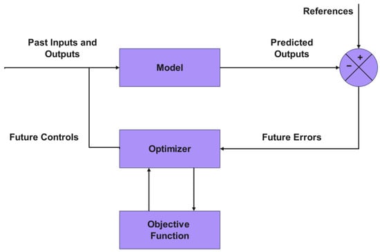
Figure 1. Basic structure of model-based optimization.

This paper is organized as follows. The Section 2 (Materials and Methods) comprises three subsections: Section 2.1 develops the multicomponent HFMM mechanistic model, including temperature-dependent viscosity and non-ideal gas behavior; Section 2.2 presents the statistical scaffold—data normalization, a normalized multiple linear regression baseline, assumption diagnostics, and multicollinearity/variable selection; and Section 2.3 details the ANFIS layer (membership functions, rule base, hybrid training, and the train/validation/test split). Section 3 presents the results, and Section 4 concludes the paper.

2. Materials and Methods

This section details the methodology used to develop a hybrid model that predicts gas separation in an HFMM. The process begins with the construction of a mathematical model based on first principles, which is rigorously validated. Subsequently, this model is used as a “virtual plant” to generate a synthetic dataset. Finally, the generated data are subjected to a thorough statistical analysis to select the most influential variables, which serve as input for training the intelligent ANFIS model. To further enhance reproducibility, Appendix A (Algorithms A1–A5) provides a series of detailed pseudocodes illustrating the implementation of the mechanistic model, data generation, statistical analysis, and the ANFIS training workflows.

2.1. Mathematical Modeling of HFMM

This model aims to describe the behavior of the separation system through mathematical relationships that account for the gas properties and the membrane’s characteristics. The most critical considerations in this model are described as follows:

• The membrane does not deform under the applied pressure. This is a simplifying assumption [3].
• Pressure drop on the permeate and retentate sides can be calculated using the Hagen-Poiseuille equation.
• Permeance of chemical species is considered constant in model validation (see Section 2.1.3).

This model is based on a set of differential equations that describe the variation of the component flow along the membrane. Equation (1) describes the rate of change in the molar flow of component i on the retentate side of the membrane in the flow direction. Equation (2) represents the rate of change in the molar flow of component i on the permeate side. Equation (3) details the pressure variation along the membrane on the retentate side, considering the dynamic viscosity of the mixture and membrane geometry. Finally, Equation (4) describes pressure variation on the permeate side; see Figure 2 [3,24].

$${\displaystyle \frac{\mathrm{d}{v}_i}{dz}}=-{Pm}_i\left(p_i^{Re}-p_i^{Pe}\right)D_o\pi N$$

(1)

$${\displaystyle \frac{\mathrm{d}{u}_i}{dz}}={Pm}_i\left(p_i^{Re}-p_i^{Pe}\right)D_o\pi N$$

(2)

$${\displaystyle \frac{dP}{dz}}={\displaystyle \frac{192N{D}_o\left(D+N{D}_o\right)RT{\mu }_{mix}^{Re}}{\pi {\left(D^2-N{D}_o^2\right)}^{3}P}}v$$

(3)

$${\displaystyle \frac{dp}{dz}}=-{\displaystyle \frac{128RT{\mu }_{mix}^{Pe}}{\pi D_i^{2}Np}}u$$

(4)

where ${Pm}_i$ is permeance of component i ${\displaystyle \frac{mol}{m^2·atm·s}}$, $p_i^{Re}$ and $p_i^{Pe}$ denote partial pressures of component in the retentate and permeate section, $atm$, $N$ is the number of tubes or fibers, $i$ is component index, $u$ is flow rate on the permeate side $\left(\mathrm{m}\mathrm{o}\mathrm{l}·\mathrm{s}\right)$ and $v$ is the flow rate on the retentate side $(\mathrm{m}\mathrm{o}\mathrm{l}·\mathrm{s}$). The internal diameter of the shell is denoted by $D$ $\left(\mathrm{m}\right)$, while $D_i$ and $D_o$ refer to the internal and external diameter of the fiber $\left(\mathrm{m}\right)$, respectively, $R$ is the universal gas constant, $T$ is the temperature, and ${\mu }_{mix}$ is the dynamic viscosity of the mixture $(\mathrm{P}\mathrm{a}·\mathrm{s})$. Superscripts $Re$ and $Pe$ are employed to denote quantities in the retentate and permeate streams, respectively. These notations are consistently applied to other variables in subsequent sections to facilitate further analyses.

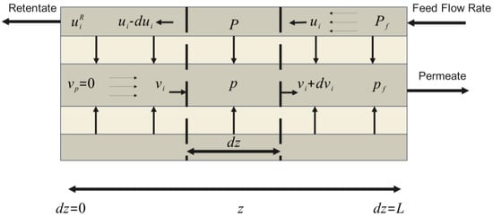
Figure 2. Countercurrent flow dynamics in an HFMM scheme.

To solve the differential equations, the MATLAB^® (version R2025b) function ode15s is used. This function employs an adaptive implicit method based on backward differentiation formulas (BDF). This approach is particularly suitable for stiff systems, as it can handle rapid and slow variations in a stable and efficient manner. First, the model equations and initial conditions were defined (see Table 3 and Table 4). Then, error tolerances and the integration interval were configured. This setup allowed for precise and stable numerical solutions for the system of interest. This model has proven valid with data from studies in [3,25,26].

Table 3. Initial conditions of the Process.

Parameter	Value	Unit
$P$	8	atm
$p$	1	atm
$T$	298.15	K
$v$	0.00135	mol/s
$D_i$	0.0002	m
$D_o$	0.0004	m
$\mathrm{N}$	3800	-
$D$	0.0381	m
$L$	0.27	m

Values of the conditions process were obtained from [5].

Table 4. Initial conditions of chemical species.

Parameter	Mole Fraction	Permeance (${\mathit{P}}_{\mathit{m}\mathit{i}}$) $\left[\mathbf{m}\mathbf{o}\mathbf{l}/({\mathbf{m}}^2·\mathbf{a}\mathbf{t}\mathbf{m}·\mathbf{s})\right]$
CO2	0.10	1.51 × 10−3
CH4	0.90	5.17 × 10−5

Values of permeance were obtained from [5].

2.1.1. Dynamic Determination of Viscosity

According to [27], the viscosity of a pure fluid can be determined using the Chapman-Enskog solution, which is based on the Boltzmann transport equation. This approach assumes that molecular interactions can be approximated by those of Lennard–Jones particles with a potential function. Dynamic viscosity of a gas ${\mu }_i$ is calculated using the kinetic theory of gases, which relates this property to temperature $T$, molar mass $M_i$, collision diameter σ, and collision integral ${\mathrm{\Omega }}_{\mu }$. The pure-component molecular weights used in the Wilke mixing rule are given in Appendix A, Table A1.

$${\mu }_i=2.669\times {10}^{-5}{\displaystyle \frac{\sqrt{T·M_i}}{{\sigma }^2·{\mathrm{\Omega }}_{\mu }}}$$

(5)

Reduced collision integral is calculated by considering the possible trajectories of particles during their approach. An empirical correlation relates ${\Omega }_{\mu }$ to temperature.

$${\Omega }_{\mu }={\displaystyle \frac{1.16145}{T^{\ast 0.14874}}}+{\displaystyle \frac{0.52487}{exp\left({0.77320T}^{\ast }\right)}}+{\displaystyle \frac{2.16178}{exp\left({2.43787T}^{\ast }\right)}}$$

(6)

where the reduced temperature $T^{\ast }$.

$$T^{\ast }={\displaystyle \frac{T}{\raisebox{1ex}{$\epsilon $}\!\left/ \!\raisebox{-1ex}{$k_B$}\right.}}$$

(7)

In this expression, $\epsilon$ is the depth of the Lennard–Jones potential well, and $k_B$ is the Boltzmann constant (1.380649 × 10⁻²³ J/K). The term ${\displaystyle \raisebox{1ex}{$\epsilon $}\!\left/ \!\raisebox{-1ex}{$k_B$}\right.}$ has units of kelvins, making $T^{\ast }$ dimensionless. Physically, $T^{\ast }$ represents the ratio of the system temperature to the characteristic energy of intermolecular interactions. The Lennard–Jones parameters adopted for collision-integral evaluations are summarized in Appendix A, Table A3.

According to [28] viscosity of a diluted gas is related to the mole fraction ${\mathrm{\chi }}_i$, and the viscosity of the diluted gas component $i$, following Wilke’s equation.

$${\mu }_{mix}=\sum _i{\displaystyle \frac{{\mathrm{\chi }}_i{\mu }_i}{\sum _j{\mathrm{\chi }}_j{\phi }_{ij}}}$$

(8)

Binary weighting factor ${\phi }_{ij}$ expressed as a function of gas viscosity and the molecular weight of component as follows:

$${\phi }_{ij}={\displaystyle \frac{{\left[1+{\left(\frac{{\mu }_i}{{\mu }_j}\right)}^{0.5}{\left(\frac{M_i}{M_j}\right)}^{0.25}\right]}^2}{{\left[8\left(1+\raisebox{1ex}{$M_i$}\!\left/ \!\raisebox{-1ex}{$M_j$}\right.\right)\right]}^{0.5}}}$$

(9)

2.1.2. Peng–Robinson Equation of State for Non-Ideal Gas Behavior

To accurately represent the non-ideal behavior of gas mixtures within the HFMM, Peng–Robinson (PR) cubic equation of state is implemented in the mathematical model. This approach allows for the calculation of the real molar volume for both the retentate and permeate streams at each spatial position along the membrane, thus providing a more rigorous description of volumetric and transport phenomena, particularly under elevated pressure conditions [29].

The Peng–Robinson equation of state is given by the following:

$$P={\displaystyle \frac{RT}{V_m-b_i}}-{\displaystyle \frac{a_i{\alpha }_i\left(T\right)}{V_m^2+2b_i{V}_m-{b_i}^2}}$$

(10)

where $P$ is the pressure, $T$ is the temperature, $V_m$ is the molar volume, and $R$ is the universal gas constant. The parameters $a_i$ and $b_i$ are determined from the critical temperature $T_c$, critical pressure $P_c$, and acentric factor $\omega$ of each species.

Computation of the parameters $a_i$ and $b_i$ for Peng–Robinson equation of state in multicomponent mixtures requires the use of appropriate mixing rules, as well as the estimation of temperature-dependent correction factors for each component.

First, for each pure component i, the parameters are defined as follows:

$$a_i=0.45724·{\displaystyle \frac{R^2{T}_{c,i}^2}{P_{c,i}}}$$

(11)

$$b_i=0.07780·{\displaystyle \frac{R{T}_{c,i}}{P_{c,i}}}$$

(12)

where $T_{c,i}$ and $P_{c,i}$ are the critical temperature and pressure of component i, respectively. The term ${\alpha }_i$ introduces temperature dependence, calculated as follows:

$${\alpha }_i\left(T\right)={\left[1+k_i\left(1-\sqrt{{\displaystyle \frac{T}{T_{c,i}}}}\right)\right]}^2$$

(13)

$$k_i=0.37464+1.54226{\omega }_i-0.26992{\omega }_i^2$$

(14)

For mixtures, global parameters $a_{mix}$ and $b_{mix}$ are obtained by classical mixing rules:

$$a_{mix}=\sum _i\sum _j{\mathrm{\chi }}_i{\mathrm{\chi }}_j\sqrt{a_i{\alpha }_i\left(T\right)a_j{\alpha }_j\left(T\right)}\left(1-k_{ij}\right)$$

(15)

$$b_{mix}=\sum _i{\mathrm{\chi }}_i{b}_i$$

(16)

In these equations, ${\mathrm{\chi }}_i$ and ${\mathrm{\chi }}_j$ are the mole fractions of components i and j, respectively. Binary interaction parameter $k_{ij}$ is an empirical coefficient used to account for non-ideal interactions between unlike pairs of molecules in the mixture, and it is usually obtained from experimental data or taken as zero in the absence of specific information.

Final values of $a_{mix}$ and $b_{mix}$ are then substituted into the cubic Peng–Robinson equation of state to compute the molar volume or compressibility factor for the mixture under the specified conditions of temperature, pressure, and composition [29].

The Peng–Robinson EoS is widely recognized as a robust model for CH₄/CO₂ mixtures under the moderate operating conditions (8 atm, 298.15 K) of this study. Its ability to provide an excellent compromise between simplicity and accuracy for CO₂-rich systems in the subcritical gas phase, with reported errors for compressibility below 1%, makes it a suitable choice for this application [30]. Furthermore, its successful implementation in recent molecular simulation studies of gas separation in membranes under comparable conditions validates its predictive capabilities [31]. The model’s robustness is also supported by its application in studies under even more demanding conditions of higher pressure [32]. The critical properties and acentric factors employed are listed in Appendix A, Table A2.

2.1.3. Permeance: Baseline Assumption and Post-Validation Exploration

The effective ${Pm}_i$ observed in operation can shift with temperature, pressure, and composition (competitive sorption, plasticization), as well as with the architecture/thickness of the selective layer and module non-idealities (pressure drops, film coefficients, non-isothermality). The specialized literature recommends, when reliable parameters are not available, conducting parametric evaluations to bound their impact on module performance and design [33].

At the material/architecture level, hollow-fiber TFC membranes with ultrathin selective layers have reported CO₂ permeances on the order of 2.6–2.7 × 10³ GPU with CO₂/N₂ selectivities of ~21; the authors note that thickness estimation assumed constant permeability despite evidence of thickness dependence and operating-condition variability, reinforcing that effective permeance is not static [34].

At the module/process level, performance depends on the integration of the separation unit (areas, stage cut, pressures) and its couplings with other units; these factors modify driving forces and fluxes, explicitly justifying the use of parametric scans when working with tabulated permeances [35].

Regarding constitutive modeling, frameworks that integrate molecular dynamic (MD)+ free-volume theory and pressure/composition-dependent permeability improve agreement with data but require nontrivial parameters; in parallel, non-ideal models (pressure-dependent permeability, substrate resistance, real-gas behavior) have been shown to reduce deviations relative to the ideal approach, supporting parametric evaluation when a full parametrization is not yet available [36].

Adopted protocol. Without introducing a new constitutive model at this stage, a post-validation exploration was carried out by varying only the CH₄ permeance in {0.1×, 1×, 10×} relative to its baseline. This approach was chosen as a first-order sensitivity analysis to evaluate the system’s response to perturbations in the less permeable species, a key factor controlling methane purity in the retentate. We acknowledge that a complete analysis would involve co-variation of CO₂ permeance to fully map the impact on selectivity, which remains a valuable direction for future studies. The scan reports eighteen outputs spanning: total volumes on each side (retentate and permeate); gas compositions on each side (CO₂ and CH₄ mole fractions); pressures on each side; component molar flows of CO₂ and CH₄ on each side; component volumes of CO₂ and CH₄ on each side; and the mixture viscosity on each side. Together, these metrics quantify the plausible impact on flow splits, compositions, and pressure profiles within a range bounded by the literature.

2.2. Statistical Method

This section details the systematic methodology, illustrated in Figure 3, used to reduce the initial set of 18 candidate predictors to a compact, high-quality subset for ANFIS modeling. The workflow is designed to ensure the final variables are not only statistically powerful but also physically meaningful.

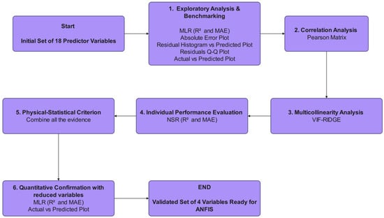
Figure 3. Statistical analysis framework for predictor dimensionality reduction.

The process begins with an Exploratory Analysis and Benchmarking phase, where a multiple linear regression (MLR) model incorporating all 18 variables is constructed. This initial model serves as a baseline, and its performance is evaluated using the coefficient of determination (R²) and mean absolute error (MAE). Its statistical validity is rigorously checked through a series of diagnostic plots, including residual analysis and Q-Q plots, to assess underlying assumptions like homoscedasticity and normality.

Subsequently, a Correlation and Multicollinearity Analysis is performed. A Pearson correlation matrix is generated to identify strong linear relationships between pairs of variables. This is complemented by a more robust multicollinearity assessment using the Variance Inflation Factor with a Ridge penalty (VIF-Ridge), which quantifies how much the variance of an estimated regression coefficient is increased due to collinearity with other predictors.

In parallel, an Individual Performance Evaluation is conducted for each predictor. By fitting a normalized simple linear regression (NSR) for each variable against the target output, we assess their individual predictive contributions, again using R² and MAE as key metrics.

The core of the selection process is the Physical-Statistical Criterion, where all the evidence is synthesized. The statistical findings—from the benchmark model, correlation matrix, VIF scores, and individual regressions—are combined with physical knowledge of the membrane separation process. This crucial step ensures that the selected variables are not just statistically independent but also mechanistically relevant.

Finally, a Quantitative Confirmation is performed. A new, reduced MLR model is built using only the four selected variables. Its performance is re-evaluated to confirm that the parsimonious model retains high predictive accuracy. This multi-stage filtering workflow systematically eliminates weak and redundant variables, guaranteeing that the final input set for the ANFIS model is both robust and interpretable.

All measurements are arranged into the standard regression form:

$$x=\left[\begin{array}{ccccc}{x}_{11}& x_{12}& x_{13}& \dots & x_{1k_0}\\ x_{21}& x_{22}& x_{23}& \dots & x_{2k_0}\\ x_{31}& x_{32}& x_{33}& \dots & x_{3k_0}\\ ⋮& ⋮& ⋮& & ⋮\\ x_{n1}& x_{n2}& x_{n3}& \dots & x_{n{k}_0}\end{array}\right]y=\left[\begin{array}{c}{y}_1\\ y_2\\ ⋮\\ y_n\end{array}\right]$$

(17)

where $n$ denotes the number of experimental observations (rows) and $k_0$ is the number of initial predictors ($k_0=18$). This succinct representation facilitates matrix-based computations and algorithmic efficiency.

To explore the relationships between variables, scatter plots are employed to visualize ordered pairs ($x_{s,q}$, $y_s$). It’s not just a graph but a visual representation of the relationship between the two variables. When most points align closely with a straight line, the correlation is classified as linear. Conversely, the correlation is considered nonlinear if the points follow a curved pattern. However, if no discernible pattern is observed among the ordered pairs, it indicates the absence of a relationship between the two variables. To depict the curve or regression line that best fits the distribution of the ordered pairs, Equation (18) is applied [36].

$$y={\beta }_0+{\beta }_1{x}_{s,1}+{\beta }_2{x}_{\mathrm{s},2}+\dots +{\beta }_q{x}_{s,q}$$

(18)

where ${\beta }_0$ is the intercept and ${\beta }_q$ are the regression coefficients associated with each predictor.

2.2.1. Data Normalization

To mitigate bias from differing variable scales, all features and the target variable are standardized to zero mean and unit variance:

$$x_{s,q}^{\left(n\right)}={\displaystyle \frac{x_{s,q}-{\mu }_{x_q}}{{\sigma }_{x_q}}},{ y}_s^{\left(n\right)}={\displaystyle \frac{y_s-{\mu }_y}{{\sigma }_y}}$$

(19)

where ${\mu }_{x_q}$ and ${\sigma }_{x_q}$ are vectors of column-wise means and standard deviations of the $q$ predictor across all $n$ samples. ${\mu }_y$ and ${\sigma }_y$ are the mean and standard deviation of the dependent variable $y$.

2.2.2. Normalized Multiple Linear Regression

A normalized multiple linear regression model was fitted to the standardized data:

$$y^{\left(n\right)}=X^{\left(n\right)}\beta$$

(20)

where $y^{\left(n\right)}$ is the vector of normalized predicted values. $X^{\left(n\right)}$ is the normalized design matrix (dimensions $n\times k_0$), with each column scaled to zero mean and unit variance, and $\beta$ is the vector (dimensions $k_0\times 1$).

2.2.3. Parameter Estimation via Gradient Descent

The coefficients $\beta$ were optimized by minimizing the mean squared error (MSE) cost function:

$$J\left(\beta \right)={\displaystyle \frac{1}{2n}}\sum _{s=1}^n{\left(y_s^{\left(n\right)}-{\widehat{y}}_s^{\left(n\right)}\right)}^2$$

(21)

Using stochastic gradient descent (SGD) with Learning rate $\alpha =0.01$, Iterations = 1000 (ensuring convergence to local minima) and an update rule according to the following:

$${\beta }^{\left(t+1\right)}={\beta }^{\left(t\right)}-\alpha {\nabla }_{\beta }J{\beta }^{\left(t\right)}$$

(22)

where the gradient $\nabla J$ is computed as follows:

$${\nabla }_{\beta }J=-{\displaystyle \frac{1}{n}}{\left(X^{\left(n\right)}\right)}^T\left(y^{\left(n\right)}-y^{\left(n\right)}\right)$$

(23)

Normalized predictions are transformed back to the original scale for direct comparison with experimental data. We evaluate performance with two metrics: the coefficient of determination (R²), defined in Equation (24), and the mean absolute error (MAE), defined in Equation (25). $R^2$ ∈ [0,1] quantifies the fraction of variance in the target explained by the model, values closer to 1 indicate a better fit. For completeness, the Pearson correlation coefficient $r$ ∈ [−1, 1] measures the strength and direction of linear association between variables [34].

$$R^2=1-{\displaystyle \frac{\sum _{s=1}^n{\left(y_s-{\widehat{y}}_s\right)}^2}{\sum _{s=1}^n{\left(y_s-\overline{y}\right)}^2}}$$

(24)

$$\mathrm{M}\mathrm{A}\mathrm{E}={\displaystyle \frac{1}{n}}\sum _{s=1}^n\left|y_s-{\widehat{y}}_s\right|$$

(25)

Normalized simple linear regression is additionally performed for each independent variable ${x;}_q^{\left(n\right)}$, repeating the same procedure and metric calculations to identify the individual contribution of each variable to the model.

2.2.4. Multicollinearity Analysis

Given that collinearity among predictors can inflate the variance of regression coefficients and undermine the numerical stability of the model. This procedure enabled the systematic elimination of highly collinear and weakly predictive variables, reducing the original pool of 18 candidate predictors to the four most informative and mutually independent inputs for ANFIS training.

Pearson’s correlation coefficients are computed according to [37] on the normalized predictor matrix $X^{\left(n\right)}$.

$${\rho }_{q\mathcal{l}}={\displaystyle \frac{\sum _{s=1}^n\left(x_{s,q}^{\left(n\right)}-{\overline{x}}_q^{\left(n\right)}\right)\left(x_{s,\mathcal{l}}^{\left(n\right)}-{\overline{x}}_{\mathcal{l}}^{\left(n\right)}\right)}{\sqrt{\sum _{s=1}^n{\left(x_{s,q}^{\left(n\right)}-{\overline{x}}_q^{\left(n\right)}\right)}^2}\sqrt{\sum _{s=1}^n{\left(x_{s,\mathcal{l}}^{\left(n\right)}-{\overline{x}}_{\mathcal{l}}^{\left(n\right)}\right)}^2}}}$$

(26)

With this, it was also possible to construct a correlation matrix which compacts all the ${\rho }_{ij}$ into a single object.

$$R_{xx}={\left[{\rho }_{q\mathcal{l}}\right]}_{q,\mathcal{l}=1}^{k_0}$$

(27)

Inspecting the correlation matrix quickly flags pairs with ${\rho }_{q\mathcal{l}}$ near 1, it remains a subjective heuristic and tells us nothing about how much multicollinearity is affecting our coefficient estimates. To quantify that impact, we turn to the variance inflation factor ${VIF}_i$ for predictor $q$, quantifying how much the variance of its estimated coefficient ${\widehat{\beta }}_q$ is inflated due to multicollinearity. Formally,

$${VIF}_q={\displaystyle \frac{Var\left(\left.{\widehat{\beta }}_q\right| with multicollinearity\right)}{Var\left(\left.{\widehat{\beta }}_q\right| no multicollinearity\right)}}={\left[{\left(R_{xx}\right)}^{-1}\right]}_{qq}$$

(28)

According to [38], ${VIF}_q$ is the $q-th$ diagonal element of ${\left(R_{xx}\right)}^{-1}$. Values ${VIF}_q$> 10 indicate severe collinearity. However, when there is severe collinearity, the correlation matrix $R_{xx}$ can become close to singular and lead to extreme or undefined values of ${VIF}_q$. To address this problem, we introduce a Ridge penalty in the collinearity diagnosis. Strictly speaking, we define the “penalized” version of the $VIF$ as follows:

$${VIF}_{q,ridge}={\left[{{\left(R_{xx}+\lambda I_{k_0}\right)}^{-1}R}_{xx}{\left(R_{xx}+\lambda I_{k_0}\right)}^{-1}\right]}_{qq}$$

(29)

Ridge penalty hyperparameter $\lambda$ controls the degree of regularization and was selected (λ = 0.03) via literature ${VIF}_{q,ridge}$. $I_{k_0}$ is the identity matrix of size $\left(k_0\times k_0\right)$, where $p$ is the number of original predictors.

2.2.5. Validation of Model Assumptions via Diagnostic Plots

To ensure that the normalized linear regression satisfies its underlying assumptions prior to ANFIS training, the following diagnostic plots are systematically generated:

• Residuals vs. Predicted Values: Plot the residual against the fitted value y_k. This visualization is used to assess homoscedasticity—constancy of error variance across the prediction range—and to detect any funnel-shaped or nonlinear patterns that would indicate model misspecification.
• Q-Q-Plot of Residuals: Construct a quantile-quantile plot comparing the empirical quantiles of the residuals to theoretical quantiles of a standard normal distribution. Close adherence of points to the 45° reference line will validate the assumption of approximate Gaussianity of the errors, which is important for subsequent inferential procedures.
• Histogram of Residuals: Generate a normalized histogram of residuals to examine the shape of their distribution—specifically symmetry, peakedness, and tail behavior. This complements the Q-Q-plot by visually confirming the presence (or absence) of skewness or heavy tails.
• Actual vs. Predicted Values: Plot observed responses $y_k$ versus predicted values ${\widehat{y}}_s$ alongside the identity line $y_s={\widehat{y}}_s$. A tight cluster of points around this line will demonstrate high overall predictive accuracy and minimal systematic bias.
• Absolute Error per Sample: Compute and plot the absolute error for each sample index. This plot helps to identify isolated outliers or regions where the model’s performance deteriorates, thereby guiding further data investigation or model refinement.

By applying these five diagnostic plots, one can confirm the validity of homoscedasticity and normality assumptions, quantify overall goodness-of-fit, and detect any influential observations that may warrant additional scrutiny before proceeding with ANFIS modeling.

2.3. Intelligent Modeling with ANFIS

The technique implemented in this study is the ANFIS, which integrates two intelligent methods: ANNs and fuzzy logic. This hybrid approach combines the learning capacity of ANNs with the interpretability of fuzzy systems, effectively addressing the limitations inherent to each individual technique as a universal approximator [39,40,41].

Classical ANFIS architecture, illustrated in Figure 4, consists of five layers:

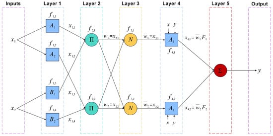
Figure 4. Architecture scheme of a two-input ANFIS network.

• Layer 1 (Membership Functions): Each input $x_j$ is fuzzified using membership functions (MFs) that transform crisp inputs into membership degrees $\mu$ ranging from 0 to 1. In this work, different membership functions were tested, such as Gaussian, triangular, sigmoidal, and bell functions. After a comparative analysis, the membership function with the best performance was the sigmoidal one, as presented and discussed later in Table 10. The sigmoidal membership function is defined as follows:

  $${\mu }_{MF}\left(x;a_{MF},c_{MF}\right)={\displaystyle \frac{1}{1+e^{-a_{MF}\left(x-c_{MF}\right)}}}$$

  (30)

where parameters $a_{MF}$ and $c_{MF}$ control the slope and center of the function, respectively.

• Layer 2 (Rule Firing Strength): Computes the firing strength $w_r$ of each fuzzy rule by aggregating membership degrees of all inputs via product:

  $$w_r=\prod _{m=1}^Q{\mu }_{MF}{A}_{rm}\left(x_m\right), r=1,\dots ,M,$$

  (31)

where $M$ is the number of fuzzy rules and $Q$ is number of inputs.

• Layer 3 (Normalization): Normalizes firing strengths:

  $${\overline{w}}_r={\displaystyle \frac{w_r}{\sum _{r^{’}=1}^M{w}_{r^{’}}}}$$

  (32)
• Layer 4 (Consequents): Each rule computes an output as a linear function of inputs weighted by ${\overline{w}}_r$:

  $$f_r={\overline{w}}_r·\left(\sum _{m=1}^Q{b}_{rm}{x}_m+c_r\right)$$

  (33)

where $b_{rm}$ and $c_r$ are consequent parameters.

• Layer 5 (Output Aggregation): Aggregates all outputs to produce final prediction:

  $$\widehat{y}=\sum _{r=1}^M{f}_r={\displaystyle \frac{\sum _{r=1}^M{w}_r{f}_r}{\sum _{r=1}^M{w}_r}}$$

  (34)

Neural network components enable continuous adjustment of weights and parameters during learning. The training method applied is a hybrid algorithm combining least squares estimation for the consequent parameters and gradient descent for nonlinear membership parameters $a_{MF}$, and $c_{MF}$ [39,40].

The error function minimized during training is the mean squared error:

$$E={\displaystyle \frac{1}{N_s}}\sum _{t=1}^{N_s}{\left(y_t-{\widehat{y}}_t\right)}^2$$

(35)

where $y_t$ and ${\widehat{y}}_t$ are actual and predicted outputs respectively. Update rule for any parameter $\alpha$ follows gradient descent:

$$\Delta \alpha =-\eta {\displaystyle \frac{\partial E_p}{\partial \alpha }}$$

(36)

with learning rate $\eta$ controlling step size.

To capture temporal dependencies, input vectors include up to 20 previous samples (lags), generating delayed inputs such as the following:

$${\widehat{v}}_{{CH}_4}^R\left(t\right)=f\left[\begin{array}{cccc}{V}^{Re}\left(t-d\right)& {Pm}_{{CH}_4}\left(t-d\right)& {{\mu }_{mix}}^{Re}\left(t-d\right)& P^{Re}\end{array}\left(t-d\right)\right], d=\mathrm{1,2},\dots ,20,$$

(37)

Data for these delayed inputs are generated from white-box membrane transport model and loaded for ANFIS training. Variable selection is performed as previously described using correlation analysis to ensure relevance and reduce redundancy.

To ensure a robust and interpretable ANFIS model, configuration and training parameters are summarized in Table 5. Model uses four selected input variables—permeance ${Pm}_{{CH}_4}$, retentate volume $V^{Re}$, retentate pressure $P^{Re}$, and retentate mixture viscosity ${\mu }_{mix}^{Re}$—with methane volume in retentate ${\widehat{v}}_{{CH}_4}^R$ as output. Temporal dependencies are incorporated by evaluating up to 20 time lags per input, allowing the model to capture the dynamic behavior of the membrane process. Sigmoidal membership functions are primarily used. Each input variable has one membership function, balancing simplicity and expressive power.

Table 5. Summary of ANFIS Model Configuration and Training Parameters.

Parameter	Description
xm	Permeance PmCH4, Retentate Volume VRe, Retentate Pressure PRe, Retentate Mixture Viscosity ${\mu }_{mix}^{Re}$
$\widehat{y}$	Methane volume in retentate ${\widehat{v}}_{{CH}_4}^R$
$d$	1 to 20 time lags to incorporate temporal dependencies in the inputs
Membership function type	Sigmoidal type
Number of Membership Functions	1 (sigmoidal)
Number or Fuzzy rules	1
Data Split	70% training, 30% testing, with no overlap between sets and cross valida-tion with 5 folds.
Training Method	Hybrid approach: linear parameter estimation via pseudoinverse combined with nonlinear optimization of parameters $a_{MF}$$\mathrm{and} c_{MF}$ by gradient descent using analytical derivatives
Parameter Initialization	Random initialization for parameters $a_{MF}$$\mathrm{and} c_{MF}$ within defined ranges.
Stopping Criteria	Maximum of 50 iterations.
Performance Metrics	Eval Time, MSE, RMSE, MAE, and coefficient of determination ($R^2$) calculated for training and testing datasets
Best Model Selection	Based on lowest test set MSE among all evaluated $d$
Validation	Graphical comparison of predicted vs. actual values in training and testing; residual error analysis

While a greater number of membership functions (MFs) can enhance an ANFIS model’s ability to capture complex nonlinearities, this typically comes at the cost of significantly increased processing time. Our findings indicate that for this application, a model with a minimal set of MFs is not only sufficient but optimal. The marginal gains in accuracy from more complex configurations did not justify the exponential increase in computational demand, rendering them impractical for the real-time estimation of CH₄ volume in the membrane retentate. Consequently, our chosen architecture strikes a robust balance between high predictive fidelity and operational efficiency.

Dataset is split into 70% training and 30% testing, maintaining strict separation to validate generalization. Training employs a hybrid method combining least squares estimation for linear consequent parameters and gradient descent for nonlinear membership parameters $a_{MF}$ and $c_{MF}$. Parameters $a_{MF}$ and $c_{MF}$ are initialized randomly within defined ranges. Training proceeds until the mean squared error (MSE) for a maximum of 50 iterations is reached. Likewise, evaluation time (Eval Time) is computed. Performance metrics (Eval Time, MSE, RMSE, MAE, and $R^2$) are computed for both training and testing sets to evaluate overall accuracy. Final model selection is based on the lowest test set MSE among all evaluated lag configurations, ensuring optimal predictive performance. Validation includes graphical comparisons of predicted versus actual values and residual analysis to confirm model reliability. This rigorous framework enables ANFIS to effectively capture the nonlinear and temporal characteristics of the HFMM. We propose implementing a real-time control scheme coupled with bio-inspired algorithms (e.g., PSO, Gray Wolf Optimizer (GWO), and DE) for process tuning and optimization [42].

3. Results

This section presents and analyzes the results obtained from the developed hybrid model, which integrates a mechanistic multicomponent transport model for hollow fiber membranes (HFMM) with an Adaptive Neuro-Fuzzy Inference System (ANFIS). The section is organized into three key subsections to demonstrate the model’s validity, the variable selection methodology, and the predictive performance of the final model.

3.1. Mathematical Modeling of HFMM Results and Validation

The accuracy and predictive capacity of the proposed mathematical model are first evaluated by comparing its results against experimental data and the reference Ko model, as shown in Figure 5. Comparison focuses on two primary performance indicators for the membrane system: methane purity (Figure 5a) and methane recovery (Figure 5b), both as functions of feed flow rate.

Figure 5. Validation of the proposed membrane model using experimental results and the Ko model. (a) Methane purity as a function of feed flow rate. (b) Methane recovery as a function of feed flow rate.

As observed in Figure 5a, all models predict a decreasing trend in methane purity with increasing feed flow rate, which is consistent with the expected reduction in separation efficiency at higher feed rates. Notably, the proposed model tracks the experimental data more closely than the Ko model, particularly at intermediate and high feed flow rates. While the Ko model significantly underestimates methane purity under these conditions, the proposed model shows smaller deviations and better alignment with experimental results, indicating a more accurate representation of the underlying transport mechanisms.

In terms of methane recovery (Figure 5b), both models reproduce the expected increasing trend as the feed flow rate rises. However, the proposed model displays improved agreement with experimental data across tested feed rates, especially at low and moderate flow values where the Ko model exhibits more pronounced discrepancies. This consistent agreement highlights the ability of the proposed model to capture both the magnitude and trend of experimental recovery data.

To provide a quantitative assessment of model accuracy, a detailed error analysis was conducted using the relative error and mean absolute error (MAE) metrics for each experimental case (Figure 6 and Figure 7). Relative error distributions for methane purity (Figure 6a) and methane recovery (Figure 6b) show that, although the Ko model achieves lower errors at the lowest feed flow rates, its accuracy diminishes as flow increases. In contrast, the proposed model shows higher errors at low flow but rapidly improves with increasing feed, outperforming the Ko model in the higher range of operational relevance.

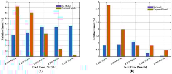
Figure 6. Relative error of the Ko model and the proposed model for the prediction of (a) methane purity and (b) methane recovery as a function of feed flow rate. Results correspond to the same experimental conditions as in Figure 5.

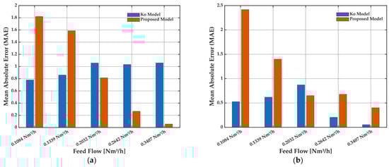
Figure 7. Mean absolute error (MAE) of the Ko model and the proposed model for the prediction of (a) methane purity and (b) methane recovery as a function of feed flow rate. Results correspond to the same experimental conditions as in Figure 5.

MAE analysis (Figure 7a,b) reinforces this observation: while the Ko model maintains a slight advantage at the lowest feed, the proposed model yields lower MAE values at moderate and high feed flows for both purity and recovery. These results confirm that the proposed model delivers robust and reliable predictions under practical operating conditions, supporting its suitability for process optimization and scale-up in HFMM.

3.2. Statistical Method Results

A comprehensive statistical analysis is carried out to evaluate the predictive performance and interrelationships of all candidate input variables considered for modeling. The objective is to identify informative and least redundant subsets of variables for training a subsequent ANFIS model. Table 6 summarizes the results of individual linear regressions, including coefficient of determination (R²), mean absolute error (MAE) and variance inflation factor ${VIF}_{q,ridge}$.

Table 6. Initial individual variable regression metrics for model reduction.

Variable	${\mathit{R}}^2$	MAE	${\mathit{V}\mathit{I}\mathit{F}}_{\mathit{q},\mathit{r}\mathit{i}\mathit{d}\mathit{g}\mathit{e}}$
Variable permeance	0.4883	3.93 × 10−6	3.70
Retentate volume	0.9998	5.47 × 10−8	0.52
Permeate volume	0.9998	5.47 × 10−8	0.52
Retentate fraction CO2	2.85 × 10−4	5.06 × 10−6	0.25
Retentate fraction CH4	2.85 × 10−4	5.06 × 10−6	0.25
Permeate fraction CO2	0.8520	1.76 × 10−6	0.24
Permeate fraction CH4	0.8520	1.76 × 10−6	0.24
Retentate pressure	0.8356	2.26 × 10−6	3.32
Permeate pressure	0.8039	2.36 × 10−6	5.62
Retentate flow CO2	0.8591	1.71 × 10−6	0.18
Retentate flow CH4	1.0000	2.21 × 10−10	0.58
Permeate flow CO2	0.8591	1.71 × 10−6	0.18
Permeate flow CH4	1.0000	2.21 × 10−10	0.58
Retentate volume CO2	0.8591	1.71 × 10−6	0.18
Permeate volume CO2	0.8591	1.71 × 10−6	0.18
Permeate volume CH4	1.0000	2.21 × 10−10	0.58
Retentate mix viscosity	0.4305	3.02 × 10−6	2.18
Permeate mix viscosity	0.8992	1.43 × 10−6	0.37

Among evaluated variables, Retentate volume and permeate volume showed near-perfect linearity ($R^2$ ≈ 0.9998–0.9999) and extremely low error (MAE = 5.47 × 10⁻⁸). However, their low ${VIF}_{q,ridge}$ values (0.52) and very high pairwise correlation (ρ > 0.93), as depicted in the Pearson correlation matrix (Figure 8), revealed significant redundancy. Including both would likely lead to multicollinearity without improving model expressiveness.

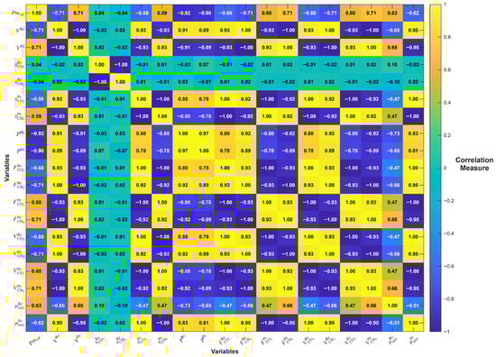
Figure 8. Pearson correlation matrix between all candidate retentate and permeate variables included in the variable selection procedure. The heatmap indicates the degree of linear relationship between each pair of variables.

Retentate Pressure demonstrated strong predictive ability ($R^2$ = 0.8356) and moderate ${VIF}_{q,ridge}$ (5.62), indicating it brings valuable and relatively unique information. Although its ${VIF}_{q,ridge}$ suggests some correlation with other inputs, it remained within an acceptable range for inclusion. On the other hand, permeance had a lower R² (0.4883) but was favored due to its meaningful physical interpretation, relatively low ${VIF}_{q,ridge}$ (3.70), and strong negative correlations with both Retentate Volume and Retentate Pressure (ρ ≈ −0.90), suggesting it captures orthogonal aspects of the system behavior.

Regarding viscosity, Permeate Mix Viscosity achieved a high R² (0.8992) and low MAE, indicating good predictive potential. However, its strong correlations with other variables (ρ > 0.9) signaled redundancy. Conversely, retentate mix viscosity showed moderate predictive performance ($R^2$ = 0.4305) and acceptable multicollinearity (${VIF}_{q,ridge}$ = 2.18) but is retained for its physical relevance and lower correlation with other selected variables (ρ < 0.5), supporting its role in improving model robustness.

The correlation matrix (Figure 8) provides a comprehensive overview of the linear interrelationships among all candidate variables. Several variables exhibited strong pairwise correlations (ρ > 0.93), indicating a high degree of redundancy in the information they convey. Notably, variables such as retentate CH₄ flow, permeate CH₄ flow, retentate CO₂ flow, and permeate CO₂ fraction were found to be tightly interrelated with other process variables—particularly retentate volume, permeate volume, and retentate pressure—all of which already captured the principal trends of the system.

Despite achieving near-perfect individual $R^2$ scores in their univariate regressions, these highly correlated variables were not selected for the final model due to their limited marginal contribution to the overall predictive power and their potential to introduce multicollinearity. This decision is further supported by their very low ${VIF}_{q,ridge}$ values (typically < 0.60), which mathematically reflect that variance in these predictors can be almost entirely explained by other variables in the model. Including such variables would not only complicate the model unnecessarily but also increase the risk of overfitting and reduce the generalizability of the final predictive tool, particularly in real-world conditions with process noise and variability.

Moreover, from a physical standpoint, flows and fractions are often dependent on the outcomes of pressure, volume, and permeance conditions, and not independent drivers of system behavior. Thus, their high correlation with physically meaningful variables such as retentate pressure and permeance reinforces the decision to exclude them in favor of more mechanistically grounded predictors.

To further validate the reliability of the selected model, residual diagnostics are conducted, as illustrated in Figure 9 and Figure 10. Figure 9a shows the absolute error per sample across the dataset. The majority of errors are small and centered, with some increase observed near sample boundaries. This pattern is consistent with edge effects, where predictive models may exhibit slightly reduced accuracy due to limited data density or extrapolation beyond the core data cloud.

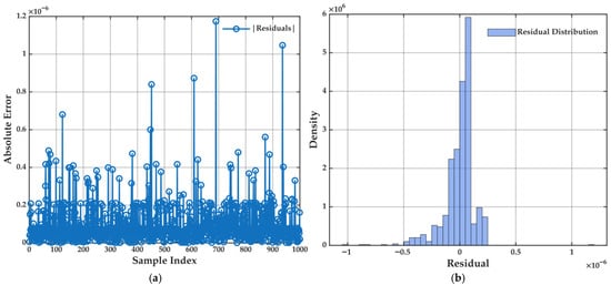
Figure 9. (a) Absolute error for each sample in the validation dataset for the multiple linear regression model. (b) Histogram of residuals showing the distribution and magnitude of errors across all samples. These visualizations provide a direct assessment of the model’s prediction accuracy and the normality of residuals, which are essential for evaluating regression model assumptions.

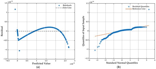
Figure 10. (a) Residuals as a function of predicted values for a multiple linear regression model, highlighting any trends or heteroscedasticity in model errors. (b) Q-Q plot of residuals, used to assess the normality of errors and the adequacy of linear model assumptions.

Figure 9b presents the histogram of residuals, which exhibits a nearly symmetric bell-shaped distribution, closely approximating normality. This supports the assumption of homoscedastic and unbiased residuals, essential conditions for the validity of linear regression estimators.

Further insight is offered by the residuals vs. predicted plot (Figure 10a), where a slight curvature is observed. While mostly centered around zero, this pattern suggests the presence of mild heteroscedasticity or a weak nonlinear component in data that a linear model may not fully capture. Nevertheless, deviation remains minor and does not compromise the model’s overall fit or its applicability for variable screening.

The scatter plot of actual versus predicted values (Figure 11a) provides a visual confirmation of the regression model’s predictive capability. Most data points align closely with the ideal 1:1 reference line, indicating a strong agreement between observed outputs and those estimated by the model. This tight clustering suggests that the regression model effectively captures dominant trends and intrinsic relationships among selected input variables. Only minimal deviations are observed at the extremes, which is typical in physicochemical models where non-linearities and edge-case behaviors may arise due to unmodeled secondary effects.

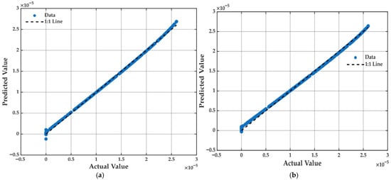
Figure 11. Comparison of actual vs. predicted values for the multiple linear regression models. (a) Performance of the model with the initial set of 18 variables. (b) Performance of the reduced model with the 4 selected variables. The dashed line indicates the ideal 1:1 relationship.

Statistical performance of regression model is further substantiated by quantitative metrics presented in Table 7. Model achieved a global coefficient of determination of $R^2$ = 0.999, indicating that 99.9% of the variability in the target variable is explained by selected predictors. Additionally, the normalized mean absolute error (MAE) is 1.292, reflecting a very low average deviation between predicted and actual values relative to the output scale. Together, these results support the robustness and high fidelity of regression models.

Table 7. Comparison of regression model performance metrics.

Metric	Value (18 Variables)	Value (4 Variables)
$R^2$	0.999	0.998
$\mathrm{M}\mathrm{A}\mathrm{E}$	1.159 × 10−7	2.279 × 10−7

To complement the visual and numerical analysis, final regression model’s structure, including linear, interaction, and higher-order terms, is presented in Table 8. This table lists the estimated coefficients ${\beta }_{\mathrm{q}}$, which quantifies the relative influence of each term used in the polynomial regression model. Inclusion of higher-order coefficients enables the model to capture subtle nonlinear dependencies without introducing excessive complexity, while preserving interpretability and numerical stability.

Table 8. The values of ${\beta }_{\mathrm{q}}$.

Parameter	MCS
${\beta }_0$	−0.035
${\beta }_1$	231
${\beta }_2$	0.162
${\beta }_3$	−0.162
${\beta }_4$	6.26 × 10−12
${\beta }_5$	−6.26 × 10−12
${\beta }_6$	5.46 × 10−8
${\beta }_7$	−5.46 × 10−8
${\beta }_8$	0.00437
${\beta }_9$	2.44 × 10−5
${\beta }_{10}$	0.00329
${\beta }_{11}$	0.00392
${\beta }_{12}$	−0.00329
${\beta }_{13}$	−0.00392
${\beta }_{14}$	0.147
${\beta }_{15}$	−0.147
${\beta }_{16}$	−0.175
${\beta }_{17}$	−0.0723
${\beta }_{18}$	0.0734

Following a comprehensive analysis that considered multiple statistical criteria—including $R^2$, MAE, ${VIF}_{k,ridge}$, and Pearson correlation coefficients—a reduced set of four variables was selected as optimal inputs for the subsequent ANFIS training process: Permeance, retentate volume, retentate pressure, and retentate mix viscosity. These variables were chosen based on their ability to capture complementary aspects of the process. Permeance represents the intrinsic transport property of the membrane, influenced by temperature, pressure, and composition. Retentate volume and retentate pressure reflect the operational state of the feed side and are strongly tied to driving forces for mass transfer. Retentate Mix Viscosity, while having moderate $R^2$, was retained for its mechanistic relevance and lower correlation with other selected inputs, thus contributing unique variance to the model. Importantly, the selected variables offer a balanced trade-off: they exhibit high predictive power, low to moderate multicollinearity (as evidenced by acceptable ${VIF}_{q,ridge}$ values), and are rooted in well-understood physical mechanisms governing membrane-based gas separation. This selection aligns with the principle of model parsimony—minimizing the number of inputs without compromising accuracy or generalizability.

Several other variables, despite exhibiting excellent individual regression metrics (e.g., Permeate Flow CH₄, Retentate Flow CO₂, Permeate Fraction CH₄), were deliberately excluded due to high pairwise correlations (ρ > 0.90), excessively low ${VIF}_{q,ridge}$ values (<0.6), or overlapping information content with already selected predictors. Additionally, some variables lacked direct mechanistic interpretability, which could hinder extrapolation or explainability of the model in broader operating domains.

Nonetheless, it is important to recognize that variable selection is inherently context-dependent. Current selection is optimized for the specific objective of training a robust, interpretable ANFIS model for this dataset and operating window. Future studies may consider evaluating alternative or expanded subsets of input variables—such as combinations including permeate mix viscosity or permeate fraction CH₄—to explore whether these configurations offer improved performance, particularly under varying process conditions, multicomponent mixtures, or in the presence of dynamic disturbances.

In summary, the selected reduced-input model demonstrates excellent agreement with observed data (see Table 9), both statistically and physically. This outcome provides a strong foundation for training intelligent models like ANFIS, while avoiding pitfalls of overfitting, multicollinearity, and loss of physical meaning.

Table 9. Criteria and Rationale for Selecting Input Variables for ANFIS Modeling.

Variable	Statistical Justification	Physical Justification	Multicollinearity	Reason for Selection
${Pm}_{{CH}_4}$	$\mathrm{Moderate} R^2$$\left(0.49\right), \mathrm{low} {VIF}_{q,ridge}$ (3.70), strong negative ρ with pressure and volume	Captures intrinsic membrane transport property	Low to moderate	Orthogonal information; essential transport parameter
$V^{Re}$	$\mathrm{Very} \mathrm{high} R^2$$\left(0.9998\right), \mathrm{low} \mathrm{MAE}, \mathrm{low} {VIF}_{q,ridge}$ (0.52)	Reflects process state, influences driving force	High with some variables	High predictive power; represents feed conditions
$P^{Re}$	$\mathrm{High} R^2$$\left(0.84\right), \mathrm{moderate} {VIF}_{q,ridge}$ (3.32)	Key driver for mass transfer, operationally controlled	Moderate	Adds unique, mechanistically important information
${\mu }_{mix}^{Re}$	Moderate $R^2$$\left(0.43\right), \mathrm{acceptable} {VIF}_{q,ridge}$ (2.18), low ρ with other selected variables	Influences mass transfer and flow resistance	Low	Mechanistic relevance; low redundancy

3.3. ANFIS Simulation Results

The dataset used for training the ANFIS model is characterized by its high complexity and variability, justifying the choice of an advanced modeling strategy.

Figure 12 presents the output variable used as the target for ANFIS training: ${\widehat{v}}_{{CH}_4}^R$ for each sample. Much like several of the input variables, the target output displays a highly scattered profile, characterized by frequent peaks and valleys and a lack of clear global trends across the dataset. Distribution is fairly symmetric, with values spanning a broad range; notably, there are no obvious outliers or missing data, though some points fall close to zero—most likely a result of diversity in simulated operating conditions or presence of measurement noise.

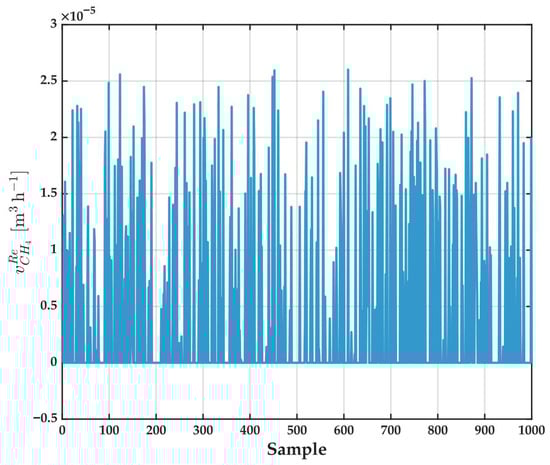
Figure 12. Experimental values of retentate ${\widehat{v}}_{{CH}_4}^{Re}$ ($\widehat{y}$) for all samples in the dataset. This variable is used as the output (target) in the ANFIS modeling.

This considerable variability in output further increases the challenge for any predictive model, as it must learn to map a set of complexes, nonlinear, and potentially noisy relationships between inputs and target values. When combined with highly variable input variables (as shown in Figure 13), this scattered output underscores the inherent complexity of the modeled gas separation process. Altogether, these figures highlight the necessity for advanced modeling strategies such as ANFIS, which are specifically designed to capture nonlinear dependencies and to provide robust predictions even in the presence of high data dispersion and noise—scenarios where traditional modeling approaches often struggle.

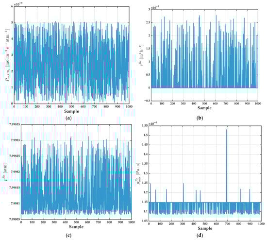
Figure 13. Input variables used for the ANFIS model: (a) ${Pm}_{{CH}_4}$ ($x_1$); (b) $V^{Re}$ ($x_2$); (c) $P^{Re}$ ($x_3$); (d) ${\mu }_{mix}^{Re}$ ($x_4$). Each plot shows the respective variable as a function of sample number for the entire dataset.

Figure 13 provides a comprehensive visualization input variables selected for the ANFIS model: (a) ${Pm}_{{CH}_4}$, (b) $V^{Re}$, (c) $P^{Re}$, and (d) ${\mu }_{mix}^{Re}$, each plotted as a function of sample number. This figure serves to illustrate both the dynamic range and variability present in the input dataset used for training and evaluating the ANFIS model.

The input variables depicted in Figure 13 show a combination of highly variable and relatively stable features, reflecting the multifaceted and sometimes unpredictable nature of real-world process data. This diversity underscores the need for robust and flexible modeling strategies—such as ANFIS—that are capable of learning complex, nonlinear, and context-dependent relationships in the presence of noisy or nonstationary inputs.

As shown, the majority of these variables exhibit marked dispersion and apparently random fluctuations throughout the entire sample set, without any discernible temporal trends, periodicities, or seasonality. This high degree of scatter highlights the complexity and nonstationary character of the system, emphasizing the modeling challenge posed by such input data.

Focusing on permeance and retentate volume, both variables display substantial variability and a wide dynamic range. These characteristics may reflect either a broad spectrum of operational scenarios—including changes in membrane properties, feed conditions, or process upsets—or the synthetic or experimental nature of the underlying dataset. The absence of smooth transitions or recurring patterns suggests that the data either samples a wide range of experimental data or intentionally incorporates variability to enhance the generality of the resulting model.

In sharp contrast, retentate pressure remains almost invariant across all samples, presenting only minor fluctuations around a stable mean value. This pattern is typical of processes where pressure is tightly controlled or regulated, ensuring that this variable does not introduce confounding effects in the modeling process. Such stability is often desirable in membrane systems to maintain separation efficiency and process safety.

Finally, retentate mix viscosity displays behavior that is generally stable, with values clustered around a central mean. Nonetheless, several isolated peaks are observed, which could be attributed to specific simulation scenarios, rare measurement anomalies, or occasional transient events in the process. These excursions, though infrequent, might provide a model with valuable information about edge-case behavior or process sensitivity.

Table 10 presents a comparative analysis considering different metrics using several ${\mu }_{MF}$, such as gaussian, sigmoidal, bell, and triangular. Likewise, datasets used are separated into 700 samples for training and 300 samples for validation. Full analysis can be consulted in Appendix A, in Table A4, Table A5 and Table A6. The results obtained show that sigmoidal ${\mu }_{MF}$ has better performance. Furthermore, sigmoidal ${\mu }_{MF}$ has only two parameters, which allows for a reduction in evaluation time.

Table 10. Comparative Analysis of Membership Function Performance in an ANFIS Model.

${\mathit{\mu }}_{\mathit{M}\mathit{F}}$	Delay	Eval Time (s)	MSETrain	RMSETrain	MAETrain	R2Train	MSETest	RMSETest	MAETest	R2Test
Gaussian	5	3.1722	7.4569 × 10−15	8.6354 × 10−8	4.3155 × 10−8	0.9998	3.4332 × 10−15	5.8594 × 10−8	3.6890 × 10−8	0.9999
Sigmoidal	4	0.0111	6.50 × 10−15	8.06 × 10−8	4.07 × 10−8	0.9998	5.83 × 10−15	7.64 × 10−8	4.39 × 10−8	0.9999
Bell	6	4.2737	7.2937 × 10−15	8.5403 × 10−8	4.4189 × 10−8	0.9998	3.8136 × 10−15	6.1755 × 10−8	3.9547 × 10−8	0.9999
Triangular	3	4.2068	5.4029 × 10−11	7.3505 × 10−6	3.328 × 10−6	−0.258	5.9828 × 10−11	7.7348 × 10−6	3.5508 × 10−6	−0.267

Table 10. Comparative Analysis of Membership Function Performance in an ANFIS Model.

${\mathit{\mu }}_{\mathit{M}\mathit{F}}$	Delay	Eval Time (s)	MSETrain	RMSETrain	MAETrain	R2Train	MSETest	RMSETest	MAETest	R2Test
Gaussian	5	3.1722	7.4569 × 10−15	8.6354 × 10−8	4.3155 × 10−8	0.9998	3.4332 × 10−15	5.8594 × 10−8	3.6890 × 10−8	0.9999
Sigmoidal	4	0.0111	6.50 × 10−15	8.06 × 10−8	4.07 × 10−8	0.9998	5.83 × 10−15	7.64 × 10−8	4.39 × 10−8	0.9999
Bell	6	4.2737	7.2937 × 10−15	8.5403 × 10−8	4.4189 × 10−8	0.9998	3.8136 × 10−15	6.1755 × 10−8	3.9547 × 10−8	0.9999
Triangular	3	4.2068	5.4029 × 10−11	7.3505 × 10−6	3.328 × 10−6	−0.258	5.9828 × 10−11	7.7348 × 10−6	3.5508 × 10−6	−0.267

Once sigmoidal ${\mu }_{MF}$ is selected, its graphical results are illustrated. Figure 14a presents a comparison between the experimental values and the predictions generated by the best ANFIS model (with $d$ = 4) for the ${\widehat{v}}_{{CH}_4}^{Re}$ across all samples. The used dataset is clearly divided by a vertical dashed line into two partitions: the initial 70% of samples are assigned to training, while the remaining 30% are reserved for testing and model validation. In both regions, model predictions (dashed lines) exhibit a remarkable alignment with actual experimental data (solid lines), capturing with high accuracy not only the general trends but also the intricate details—such as sharp peaks and deep valleys—that characterize the output signal.

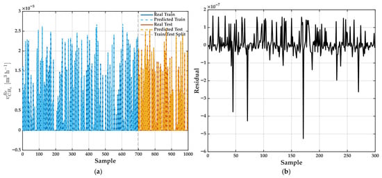
Figure 14. (a) Comparison between experimental (Real Train: solid blue line; Real Test: solid orange line) and predicted values (Predicted Train: dashed blue line; Predicted Test: dashed orange line) of ${\widehat{v}}_{{CH}_4}^{Re}$ obtained by the best ANFIS model ($d$ = 4). The model is trained using 70% of the data and tested on the remaining 30%. Vertical dashed line indicates train/test split. (b) Residuals (prediction errors) for test set using best ANFIS model ($d$ = 4).

A closer inspection reveals that the ANFIS model preserves this high fidelity even in segments where the process response is particularly volatile or shows abrupt fluctuations. This is especially noteworthy, as such regions typically pose significant challenges for both conventional and data-driven modeling approaches, often resulting in loss of precision or the introduction of systematic errors. Model’s consistent performance throughout both smooth and highly variable intervals suggests that it is not simply memorizing data (overfitting) but rather learning and internalizing the underlying process dynamics.

Moreover, near-perfect overlap between real and predicted curves in both training and testing subsets underscores the model’s ability to generalize to previously unseen data, which is critical for practical applications in real-world systems. This level of predictive accuracy, even under challenging conditions, highlights the effectiveness of the ANFIS approach when dealing with complex systems where interactions among variables are nonlinear, time-dependent, and potentially obscured by noise.

To complement this visual assessment, Figure 14b provides an in-depth analysis of the model’s predictive accuracy by displaying the residuals— pointwise errors between experimental and predicted values—over the entire test set. The vast majority of these residuals remain tightly clustered around zero, with only isolated instances where more substantial errors occur. Lack of persistent trends, recurring spikes, or clusters of large errors throughout the sample range indicates that the model does not introduce bias, nor does it fail systematically under any particular set of operating conditions. Such a balanced distribution of errors is a desirable attribute, as it suggests that the model’s occasional larger deviations are more likely attributable to inherent data noise or rare process events rather than to structural deficiencies in the model itself.

Another important aspect is that, despite the high degree of scatter and the presence of noise in both input and output variables (as illustrated in Figure 12 and Figure 13), the ANFIS model maintains robustness and does not suffer from degradation in predictive quality as data complexity increases. This robustness is particularly valuable in industrial settings, where sensor noise, process disturbances, and changes in operating regimes are common and can easily compromise the performance of less adaptive models.

Across all tested $d$ (see Table 11), ANFIS models achieved outstanding accuracy, with R² values of 0.999 for both subsets and extremely low error metrics (on the order of 10⁻¹⁵ for MSE and less than 10⁻⁷ for RMSE). These results reflect both the suitability of selected variables and the ability of ANFIS to model complex, nonlinear processes.

Table 11. Performance metrics for ANFIS models at different times, $d$. Metrics Eval Time, MSE, RMSE, MAE, R2 for both the training and test datasets. Best result is highlighted in bold.

Delay	Eval Time (s)	MSETrain	RMSETrain	MAETrain	R2Train	MSETest	RMSETest	MAETest	R2Test
1	0.0077	6.5682 × 10−15	8.1045 × 10−8	4.0207 × 10−8	0.9998	5.8827 × 10−15	7.6699 × 10−8	4.3855 × 10−8	0.9999
2	0.0078	6.5491 × 10−15	8.0926 × 10−8	4.0288 × 10−8	0.9998	5.8646 × 10−15	7.6581 × 10−8	4.3781 × 10−8	0.9999
3	0.0089	6.5080 × 10−15	8.0672 × 10−8	4.0305 × 10−8	0.9998	5.8353 × 10−15	7.6389 × 10−8	4.3838 × 10−8	0.9999
4	0.0111	6.4958 × 10−15	8.0597 × 10−8	4.0715 × 10−8	0.9998	5.8345 × 10−15	7.6384 × 10−8	4.3929 × 10−8	0.9999
5	0.0143	6.4895 × 10−15	8.0557 × 10−8	4.0732 × 10−8	0.9998	5.8459 × 10−15	7.6459 × 10−8	4.4128 × 10−8	0.9999
6	0.0142	6.4649 × 10−15	8.0405 × 10−8	4.0680 × 10−8	0.9998	5.8456 × 10−15	7.6457 × 10−8	4.4327 × 10−8	0.9999
7	0.0158	6.4602 × 10−15	8.0375 × 10−8	4.0815 × 10−8	0.9998	5.8696 × 10−15	7.6613 × 10−8	4.4559 × 10−8	0.9999
8	0.0188	6.4516 × 10−15	8.0322 × 10−8	4.1009 × 10−8	0.9998	5.9111 × 10−15	7.6884 × 10−8	4.4614 × 10−8	0.9999
9	0.0192	6.4121 × 10−15	8.0076 × 10−8	4.1117 × 10−8	0.9998	5.8620 × 10−15	7.6564 × 10−8	4.4542 × 10−8	0.9999
10	0.0215	1.7664 × 10−13	4.2029 × 10−7	1.9986 × 10−7	0.9958	2.3289 × 10−13	4.8259 × 10−7	2.5229 × 10−7	0.9952
11	0.0234	1.9624 × 10−12	1.4008 × 10−6	6.2475 × 10−7	0.9536	2.3208 × 10−12	1.5234 × 10−6	7.6129 × 10−7	0.9522
12	0.0260	3.4528 × 10−11	5.8760 × 10−6	2.5711 × 10−6	0.1844	4.2499 × 10−11	6.5192 × 10−6	3.2217 × 10−6	0.1263
13	0.0274	5.0096 × 10−11	7.0779 × 10−6	3.0953 × 10−6	−0.1821	6.1502 × 10−11	7.8423 × 10−6	3.8721 × 10−6	−0.2644
14	0.0289	4.8944 × 10−11	6.9960 × 10−6	3.0619 × 10−6	−0.1536	6.0004 × 10−11	7.7462 × 10−6	3.8249 × 10−6	−0.2336
15	0.0408	1.7002 × 10−12	1.3039 × 10−6	5.8830 × 10−7	0.9603	2.0688 × 10−12	1.4383 × 10−6	7.2201 × 10−7	0.9568
16	0.0436	5.1784 × 10−11	7.1961 × 10−6	3.1518 × 10−6	−0.2097	6.1707 × 10−11	7.8554 × 10−6	3.8599 × 10−6	−0.2889
17	0.0346	9.3228 × 10−12	3.0533 × 10−6	1.3496 × 10−6	0.7825	1.1175 × 10−11	3.3429 × 10−6	1.6535 × 10−6	0.7666
18	0.0360	8.3914 × 10−12	2.8968 × 10−6	1.2885 × 10−6	0.8044	9.7818 × 10−12	3.1276 × 10−6	1.5537 × 10−6	0.7957
19	0.0381	4.9418 × 10−8	2.2230 × 10−4	9.8204 × 10−5	−1150.4074	5.8296 × 10−8	2.4145 × 10−4	1.1864 × 10−4	−1213.9289
20	0.0397	3.9225 × 10−11	6.2629 × 10−6	2.7594 × 10−6	0.0871	4.6493 × 10−11	6.8186 × 10−6	3.3415 × 10−6	0.0311

As $d$ increases from 1 to 20, only minor variations are observed in the error metrics. MSE and MAE remain low and relatively stable for $d$ between 1 and 9, with a gradual increase in error from $d$ = 10 onward. Best predictive performance in the test set is obtained with a $d$ of 4, where the lowest MSE and MAE values are recorded. This indicates that incorporating a moderate memory of previous samples enables the model to optimally capture temporal dependencies without introducing unnecessary complexity or overfitting.

To rigorously evaluate the model’s generalization capability, a cross-validation was performed, with the results summarized in Table 12. This analysis confirms the exceptional predictive performance and stability of the ANFIS architecture.

Table 12. Performance metrics for ANFIS models with different time $d$ using cross-validation. Metrics Eval Time, MSE, RMSE, MAE, R² for both the training and test datasets. The best result is highlighted in bold.

Delay	Eval Time (s)	MSE Test (Avg ± Std)	RMSE Test (Avg ± Std)	MAE Test (Avg ± Std)	R2 Test (Avg ± Std)
1	0.0021	7.735 × 10−15 ± 3.356 × 10−15	8.642 × 10−8 ± 1.824 × 10−8	3.890 × 10−8 ± 4.691 × 10−9	0.9998 ± 0.0001
2	0.0014	8.301 × 10−15 ± 3.746 × 10−15	8.957 × 10−8 ± 1.865 × 10−8	4.036 × 10−8 ± 2.922 × 10−9	0.9998 ± 0.0001
3	0.0018	7.256 × 10−15 ± 4.286 × 10−15	8.276 × 10−8 ± 2.255 × 10−8	4.006 × 10−8 ± 2.732 × 10−9	0.9998 ± 0.0001
4	0.0027	8.387 × 10−15 ± 3.983 × 10−15	8.945 × 10−8 ± 2.193 × 10−8	4.145 × 10−8 ± 3.036 × 10−9	0.9998 ± 0.0001
5	0.0026	7.565 × 10−15 ± 3.810 × 10−15	8.472 × 10−8 ± 2.202 × 10−8	4.098 × 10−8 ± 3.133 × 10−9	0.9998 ± 0.0001
6	0.0030	7.581 × 10−15 ± 4.334 × 10−15	8.470 × 10−8 ± 2.257 × 10−8	4.087 × 10−8 ± 4.583 × 10−9	0.9998 ± 0.0001
7	0.0032	7.568 × 10−15 ± 3.840 × 10−15	8.508 × 10−8 ± 2.030 × 10−8	4.187 × 10−8 ± 2.673 × 10−9	0.9998 ± 0.0001
8	0.0034	7.524 × 10−15 ± 3.731 × 10−15	8.462 × 10−8 ± 2.132 × 10−8	4.169 × 10−8 ± 3.158 × 10−9	0.9998 ± 0.0001
9	0.0037	8.011 × 10−15 ± 3.050 × 10−15	8.812 × 10−8 ± 1.754 × 10−8	4.281 × 10−8 ± 3.534 × 10−9	0.9998 ± 0.0001
10	0.0040	7.718 × 10−15 ± 3.231 × 10−15	8.649 × 10−8 ± 1.720 × 10−8	4.302 × 10−8 ± 2.830 × 10−9	0.9998 ± 0.0001
11	0.0044	6.149 × 10−12 ± 9.529 × 10−12	1.681 × 10−6 ± 2.039 × 10−6	8.087 × 10−7 ± 1.019 × 10−6	0.8764 ± 0.1741
12	0.0049	1.210 × 10−11 ± 1.793 × 10−11	2.259 × 10−6 ± 2.957 × 10−6	1.056 × 10−6 ± 1.399 × 10−6	0.7511 ± 0.3601
13	0.0054	1.184 × 10−11 ± 1.856 × 10−11	2.788 × 10−6 ± 2.255 × 10−6	1.253 × 10−6 ± 9.445 × 10−7	0.7058 ± 0.4847
14	0.0056	1.527 × 10−11 ± 1.386 × 10−11	3.359 × 10−6 ± 2.234 × 10−6	1.573 × 10−6 ± 1.078 × 10−6	0.6688 ± 0.2729
15	0.0060	1.627 × 10−10 ± 3.052 × 10−10	9.206 × 10−6 ± 9.873 × 10−6	4.044 × 10−6 ± 4.061 × 10−6	−3.3766 ± 8.4932
16	0.0066	3.130 × 10−11 ± 2.162 × 10−11	5.273 × 10−6 ± 2.088 × 10−6	2.396 × 10−6 ± 9.865 × 10−7	0.2707 ± 0.4788
17	0.0067	3.619 × 10−11 ± 1.319 × 10−11	5.938 × 10−6 ± 1.077 × 10−6	2.706 × 10−6 ± 4.863 × 10−7	0.1866 ± 0.2695
18	0.0070	2.568 × 10−11 ± 2.965 × 10−11	4.008 × 10−6 ± 3.468 × 10−6	1.840 × 10−6 ± 1.585 × 10−6	0.4516 ± 0.6191
19	0.0074	7.472 × 10−10 ± 1.654 × 10−9	1.424 × 10−5 ± 2.608 × 10−5	6.721 × 10−6 ± 1.244 × 10−5	−14.9436 ± 35.2595
20	0.0082	9.743 × 10−12 ± 1.215 × 10−11	2.649 × 10−6 ± 1.846 × 10−6	1.213 × 10−6 ± 7.754 × 10−7	0.7801 ± 0.2853

The results demonstrate outstanding and consistent accuracy for models with short time lags. For delays between $d$ = 1 and $d$ = 10, the models achieved average R² values of 0.9998 and Mean Square Errors (MSE) on the order of 10−15, indicating high reliability regardless of the data partition.

However, a drastic degradation in performance is observed for lags greater than 10 ($d$ > 10), where the R² decreases and errors increase by several orders of magnitude. This behavior suggests that an excess of historical information introduces noise, causing model instability and a loss of its generalization capability.

Based on this analysis, the model with a time lag of $d$ = 3 is identified as the optimal configuration. It offers the best balance between near-perfect accuracy, demonstrated by the lowest average MSE (7.256 × 10⁻¹⁵) and computational efficiency, validating its robustness for real-time prediction and control applications.

The architecture of the optimal ANFIS model, corresponding to a time lag of $d$ = 3, is illustrated in Figure 15. This structure is notable for its parsimony; although neuro-fuzzy systems can house significant complexity, the preceding statistical analysis demonstrated that a model with a single fuzzy rule (Equation (38)) was sufficient to capture the dynamic process with exceptional precision. The rule follows a first-order Sugeno structure, where if the four input variables (Permeance, Retentate Volume, Retentate Pressure, and Retentate Mix Viscosity) meet their respective membership functions, then the output (methane volume in the retentate) is calculated as a linear combination of those inputs. The fact that such a simple architecture achieves such high performance underscores the effectiveness of the variable selection and the synergy between the mechanistic model and the neuro-fuzzy approach.

$$\begin{gathered} \mathrm{I}\mathrm{F}{x}_{1 }\mathrm{i}\mathrm{s} {MF}_1 \mathrm{A}\mathrm{N}\mathrm{D} x_{2 }\mathrm{i}\mathrm{s} {MF}_2 \mathrm{A}\mathrm{N}\mathrm{D} x_{3 }\mathrm{i}\mathrm{s} {MF}_3 \mathrm{A}\mathrm{N}\mathrm{D} x_{4 }\mathrm{i}\mathrm{s} {MF}_{4 }\mathrm{T}\mathrm{H}\mathrm{E}\mathrm{N} \\ y=b_1{x}_{1 }+b_2{x}_{2 }+b_3{x}_3+b_4{x}_{4 }+c_1 \end{gathered}$$

(38)

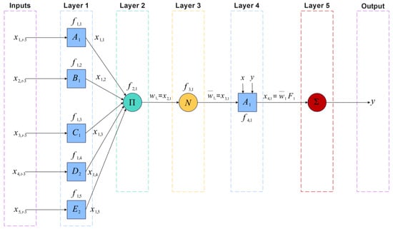
Figure 15. Architecture of the single-rule ANFIS model for the optimal time lag (d = 3). This title specifies that the diagram represents the structure of the best-performing model identified through cross-validation, which uses a single fuzzy rule and a time delay of three samples.

To conclusively validate the robustness of this optimal model, Table 13 presents a detailed breakdown of the performance metrics for each of the five folds of the cross-validation. The results demonstrate remarkable stability and consistency. Across all folds, the coefficient of determination (R²) remains above 0.999, while the Mean Squared Error (MSE) and Mean Absolute Error (MAE) stay at extremely low orders of magnitude (10⁻¹⁵ and 10⁻⁸, respectively). The minimal deviation in these metrics across the different test subsets confirms that the model’s superior performance is not an artifact of a fortunate data partition but the result of a genuine generalization capability.

Table 13. Cross-validation performance metrics by fold for the optimal ANFIS model ($d$ = 3).

Fold	MSE Test	RMSE Test	MAE Test	R2 Test
1	6.781 × 10−15	8.235 × 10−8	4.209 × 10−8	0.9999
2	3.406 × 10−15	5.836 × 10−8	3.532 × 10−8	0.9999
3	6.108 × 10−15	7.815 × 10−8	3.996 × 10−8	0.9999
4	1.430 × 10−14	1.196 × 10−7	4.307 × 10−8	0.9996
5	7.742 × 10−15	8.799 × 10−8	4.179 × 10−8	0.9998

Figure 16a illustrates the evolution of the two main learning algorithm parameters: the step size (k), which is updated using heuristic rules proposed by Jang in [41], and the learning rate (η). Unlike an approach with fixed parameters, a dynamic behavior is observed. The learning rate (η), associated with the gradient descent method for nonlinear parameters, exhibits significant fluctuations throughout the 50 epochs. This indicates that the algorithm actively adjusts the magnitude of the updates to efficiently navigate the error surface. Simultaneously, the step size (k), associated with the adjustment of the linear parameters, decreases in a stepwise fashion, suggesting progressive stabilization as the model approaches the optimal solution.

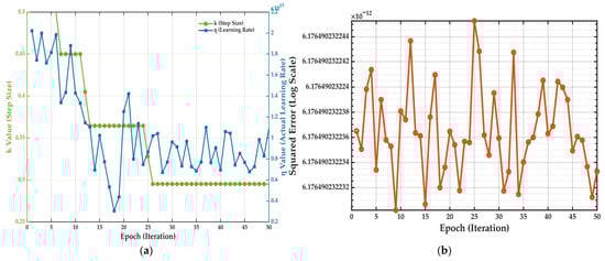
Figure 16. (a) Evolution of the adaptive step size (k) and learning rate (η) across 50 training epochs. (b) Squared error per epoch, illustrating the model’s convergence behavior.

Meanwhile, Figure 16b shows the evolution of the squared error per epoch. Notably, the error converges almost instantaneously to an extremely low error valley (on the order of 10⁻¹²) without showing a typical steep descent curve. The low-amplitude, high-frequency fluctuations observed from that point onward do not indicate instability but are a direct reflection of the micro-adjustments made by the adaptive learning rate shown in Figure 16a. This behavior demonstrates that after a very rapid initial convergence, the algorithm continues a fine-tuning process to ensure the model settles in a deep and stable error minimum.

Taken together, both graphs confirm the efficiency and sophistication of the hybrid training method. The adaptive mechanism allows for swift convergence and precise parameter adjustment, which justifies the superior performance and robustness of the final selected model.

Figure 17 provides a compelling visual validation of the ANFIS model’s performance. It displays a near-perfect superposition of the actual methane volume in the retentate (solid blue line) and the values predicted by the model (dashed yellow line). This exceptional fit is maintained across the entire dataset, capturing with high fidelity not only the general trends but also the abrupt fluctuations and volatility of the process.

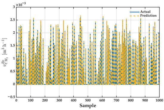
Figure 17. Validation of the Optimal ANFIS Model’s Predictive Performance. The plot shows the superposition of the actual (solid blue) and model-predicted (dashed yellow) values for the methane volume ${\widehat{v}}_{{CH}_4}^{Re}$ in the retentate across the entire dataset, demonstrating a near-perfect fit.

The model’s ability to precisely track the sharp peaks and valleys demonstrates that it has successfully learned the complex, nonlinear dynamics of the membrane system. This excellent visual agreement is the graphical representation of the quantitative metrics previously reported, such as a coefficient of determination (R²) close to 0.999. In summary, the plot confirms the model’s robustness and high precision.

The viability of a model for real-time applications depends not only on its accuracy but also on its computational efficiency. Therefore, the inference latency of the optimal ANFIS model was evaluated, and the results are presented in Table 14. This analysis quantifies the time required by the model to generate predictions as a function of the number of samples processed simultaneously (in a batch).

Table 14. Inference Time Analysis for the Optimal ANFIS Model.

# Samples	Average Time	Standard Deviation	Minimum Time	Maximum Latency
1	0.3930 ms	0.0000 ms	0.3930 ms	0.3930 ms
10	0.1252 ms	0.2486 ms	0.0080 ms	0.8190 ms
100	0.0085 ms	0.0025 ms	0.0080 ms	0.0250 ms
500	0.0086 ms	0.0023 ms	0.0070 ms	0.0370 ms

For a single sample, the model demonstrates exceptional responsiveness, generating a prediction in just 0.3930 ms. This speed is fundamental for control systems that require immediate decisions. A key finding is the notable gain in efficiency achieved through batch processing; as the number of samples increases, the average inference time per sample decreases drastically. Specifically, when processing a batch of 100 samples, the average time per prediction is reduced to 0.0085 ms, representing an improvement of over 97% compared to individual processing.

It is observed that performance stabilizes for batches of 100 and 500 samples, indicating that the model’s maximum computational efficiency has been reached under these conditions. In addition to speed, the stability of the performance is notable, as the standard deviation significantly decreases for larger batches, which confirms that the prediction times are highly consistent and reliable. Taken together, these results confirm that the ANFIS model is computationally efficient, validating its implementation in real-time monitoring and control applications where response speed is a critical factor.

4. Conclusions

In this work, it has been demonstrated that combining a first-principles transport model with an ANFIS produces a tool that is both powerful and interpretable for modeling CH₄/CO₂ separation in HFMM. By systematically reducing eighteen candidate predictors to only four—permeance, retentate volume, retentate pressure, and mixture viscosity of the retentate—via Pearson correlation, VIF (with ridge regularization), and normalized regression diagnostics, it is also ensured a parsimonious input set that balances physical insight and statistical rigor. This hybrid framework not only preserves mechanistic transparency but also injects flexibility of data-driven learning, so that the “fuzzy” part of ANFIS remains strictly in the logic layer—never clouding our understanding of underlying physics!

While an initial analysis training on 70% of the simulated dataset and validating on the remaining 30% suggested the best ANFIS configuration was the one with a time lag of $d$ = 4, a more robust cross-validation was performed to get a more reliable estimate of the model’s generalization capability. This more rigorous method revealed that the model with a time lag of $d$ = 3 was the true optimum, and this final configuration achieved an R² of 0.999 and an RMSE below 8 × 10⁻⁸ m³/h for retentate methane volume prediction. Such near-perfect agreement, across both smooth regimes and abrupt dynamics, confirms that the model is anything but “fuzzy” in its accuracy.

Validity is restricted by the assumptions and the training domain. For validation, permeances were assumed constant; strong dependencies on T, P, or composition (e.g., competitive sorption, plasticization, aging/moisture) or module non-idealities (maldistribution, external film resistances) not explicitly parameterized can degrade accuracy. The hydrodynamics are 1D and laminar (Hagen–Poiseuille) with non-deformable fibers; deviations are expected under transitional/turbulent flow, slip/Knudsen regimes at very low pressure, or fiber compaction at high pressure drop. PR-EOS and Wilke/Chapman–Enskog viscosity models are adequate across broad ranges but may require corrections near critical regions, under incipient condensation, or for strongly associating/heavy/impure mixtures (e.g., C3+, H₂S, high humidity). The ANFIS was trained on physics-generated data. While performance was initially evaluated with a 70/30 train/test split, a cross-validation was also implemented to ensure a more reliable estimate of the model’s generalization capability. To this end, future work will focus on the development of a pilot-scale plant to obtain our own experimental data. This will allow for a direct validation of the model’s generalization to real-world conditions and enable further calibration of the intelligent system, bridging the gap between simulation and industrial application.

From an applied standpoint, this hybrid approach fully aligns with Industry 4.0 objectives: it reduces parameter uncertainty, adapts in real time to process disturbances, and serves as an interpretable “soft sensor” for advanced monitoring and control.

In this context, the interpretability of the ANFIS component provides actionable insight for process engineers in two key ways. First, as a decision-support tool, the ANFIS model distills the complex set of differential equations from the mechanistic model into a single, intuitive “IF-THEN” fuzzy rule. This rule acts as a transparent soft sensor, allowing an operator without modeling expertise to gain a qualitative, cause-and-effect understanding of how input variables (such as permeance or retentate pressure) influence the final methane volume, thereby guiding operational adjustments. Second, its simplicity and high computational speed make it the foundation for advanced process optimization. The model is designed to be integrated into an optimization loop coupled with bio-inspired algorithms, using its predictions within a cost function to determine the optimal operating conditions that maximize methane purity or recovery.

That a single membership function per input sufficed to capture complex nonlinearities underscores the wisdom of marrying white-box equations with neuro-fuzzy learning—delivering high precision without unnecessary model bloat. Moreover, this white-box model can be substituted by a data-collection system in physical plants, enabling empirical calibration and adjustment of the Intelligent Model under real operating conditions.

Looking ahead, integrating this ANFIS-enhanced model into multi-objective optimization routines or closed-loop control schemes promises to further boost the efficiency and resilience of gas separation processes. Specifically, and as a key priority for our next investigation, we will conduct the sensitivity analysis on fiber compaction. This analysis will quantify how potential reductions in fiber diameter impact pressure drop and CH₄ recovery, thereby directly addressing the model’s utility for industrial scale-up. Future work could also explore online parameter adaptation under real plant noise, extension to multicomponent mixtures beyond CH₄/CO₂, and pilot-scale validation.

References

- Agwu, O.E.; Alatefi, S.; Azim, R.A.; Alkouh, A. Applications of artificial intelligence algorithms in artificial lift systems: A critical review. Flow Meas. Instrum. 2024, 97, 102613. [Google Scholar] [CrossRef]
- Lu, H.; Guo, L.; Azimi, M.; Huang, K. Oil and gas 4.0 era: A systematic review and outlook. Comput. Ind. 2019, 111, 68–90. [Google Scholar] [CrossRef]
- Chu, Y.; Lindbråthen, A.; Lei, L.; He, X.; Hillestad, M. Mathematical modeling and process parametric study of CO2 removal from natural gas by hollow fiber membranes. Chem. Eng. Res. Des. 2019, 148, 45–55. [Google Scholar] [CrossRef]
- Gu, B. Mathematical modelling and simulation of CO2 removal from natural gas using hollow fibre membrane modules. Korean Chem. Eng. Res. 2022, 60, 51–61. [Google Scholar] [CrossRef]
- Ko, D. Development of a dynamic simulation model of a hollow fiber membrane module to sequester CO2 from coalbed methane. J. Membr. Sci. 2018, 546, 258–269. [Google Scholar] [CrossRef]
- Gbadamosi, A.O.; Junin, R.; Manan, M.A.; Agi, A.; Yusuff, A.S. An overview of chemical enhanced oil recovery: Recent advances and prospects. Int. Nano Lett. 2019, 9, 171–202. [Google Scholar] [CrossRef]
- Baghban, A.; Azar, A.A. ANFIS modeling of CO2 separation from natural gas using hollow fiber polymeric membrane. Energy Sources Part A Recovery Util. Environ. Eff. 2017, 40, 193–199. [Google Scholar] [CrossRef]
- Rezakazemi, M.; Azarafza, A.; Dashti, A.; Shirazian, S. Development of hybrid models for prediction of gas permeation through FS/POSS/PDMS nanocomposite membranes. Int. J. Hydrogen Energy. 2018, 43, 17283–17294. [Google Scholar] [CrossRef]
- Alibak, A.H.; Alizadeh, S.M.; Davodi Monjezi, S.; Alizadeh, A.; Alobaid, F.; Aghel, B. Developing a hybrid neuro-fuzzy method to predict carbon dioxide (CO2) permeability in mixed matrix membranes containing SAPO-34 zeolite. Membranes 2022, 12, 1147. [Google Scholar] [CrossRef]
- Abdollahi, S.A.; Ranjbar, S.F. Modeling the CO2 separation capability of poly(4-methyl-1-pentane) membrane modified with different nanoparticles by artificial neural networks. Sci. Rep. 2023, 13, 8812. [Google Scholar] [CrossRef]
- Kim, N.E.; Basak, J.K.; Kim, H.T. Application of hollow fiber membrane for the separation of carbon dioxide from atmospheric air and assessment of its distribution pattern in a greenhouse. Atmosphere 2023, 14, 299. [Google Scholar] [CrossRef]
- Ames, A.; Flores-López, L.Z.; Rogel-Hernandez, E.; Castro, J.R.; Wakida, F.T.; Espinoza-Gomez, H. Electro-cross-flow ultrafiltration system for the rejection of nickel ions from aqueous solution, and Sugeno fuzzy model simulation. Chem. Eng. Commun. 2015, 202, 936–945. [Google Scholar] [CrossRef]
- Fathi, S.; Rezaei, A.; Mohadesi, M.; Nazari, M. PSO-ANFIS and ANN modeling of propane/propylene separation using Cu-BTC adsorbent. J. Chem. Pet. Eng. 2019, 53, 191–201. [Google Scholar] [CrossRef]
- Dashti, A.; Raji, M.; Azarafza, A.; Rezakazemi, M.; Shirazian, S. Computational simulation of CO2 sorption in polymeric membranes using genetic programming. Arab. J. Sci. Eng. 2020, 45, 7655–7666. [Google Scholar] [CrossRef]
- Babanezhad, M.; Nakhjiri, A.T.; Shirazian, S. Changes in the number of membership functions for predicting the gas volume fraction in two-phase flow using grid partition clustering of the ANFIS method. ACS Omega 2020, 5, 16284–16291. [Google Scholar] [CrossRef]
- Pishnamazi, M.; Babanezhad, M.; Nakhjiri, A.T.; Rezakazemi, M.; Marjani, A.; Shirazian, S. ANFIS grid partition framework with difference between two sigmoidal membership functions structure for validation of nanofluid flow. Sci. Rep. 2020, 10, 15395. [Google Scholar] [CrossRef]
- Sodeifian, G.; Niazi, Z. Prediction of CO2 absorption by nanofluids using artificial neural network modeling. Int. Commun. Heat Mass Transf. 2021, 123, 105193. [Google Scholar] [CrossRef]
- Aghilesh, K.; Mungray, A.; Agarwal, S.; Ali, J.; Garg, M.C. Performance optimisation of forward-osmosis membrane system using machine learning for the treatment of textile industry wastewater. J. Clean. Prod. 2021, 289, 125690. [Google Scholar] [CrossRef]
- Ansarian, O.; Beiki, H. Nanofluids application to promote CO2 absorption inside a bubble column: ANFIS and experimental study. Int. J. Environ. Sci. Technol. 2022, 19, 9979–9990. [Google Scholar] [CrossRef]
- Banik, A.; Majumder, M.; Biswal, S.K.; Bandyopadhyay, T.K. Polynomial neural network-based group method of data handling algorithm coupled with modified particle swarm optimization to predict permeate flux (%) of rectangular sheet-shaped membrane. Chem. Pap. 2022, 76, 79–97. [Google Scholar] [CrossRef]
- Nait Amar, M.; Djema, H.; Belhaouari, S.B.; Zeraibi, N. Toward robust models for predicting carbon dioxide absorption by nanofluids. Greenh. Gases Sci. Technol. 2022, 12, 537–551. [Google Scholar] [CrossRef]
- Cooley, I.; Boobier, S.; Hirst, J.D.; Besley, E. Machine learning insights into predicting biogas separation in metal–organic frameworks. Commun. Chem. 2024, 7, 102. [Google Scholar] [CrossRef] [PubMed]
- Amirkhani, F.; Dashti, A.; Abedsoltan, H.; Mohammadi, A.H.; Zhou, J.L.; Altaee, A. Modeling and estimation of CO2 capture by porous liquids through machine learning. Sep. Purif. Technol. 2025, 359, 130445. [Google Scholar] [CrossRef]
- Chen, B.; Dai, Y.; Ruan, X.; Xi, Y.; He, G. Integration of molecular dynamic simulation and free volume theory for modeling membrane VOC/gas separation. Front. Chem. Sci. Eng. 2018, 12, 296–305. [Google Scholar] [CrossRef]
- Medi, B.; Vesali-Naseh, M.; Haddad-Hamedani, M. A generalized numerical framework for solving cocurrent and counter-current membrane models for gas separation. Heliyon 2022, 8, e09053. [Google Scholar] [CrossRef]
- Khalilpour, R.; Abbas, A.; Lai, Z.; Pinnau, I. Analysis of hollow fibre membrane systems for multicomponent gas separation. Chem. Eng. Res. Des. 2013, 91, 332–347. [Google Scholar] [CrossRef]
- Wang, Z.; Han, Y.; Cao, W. Simplified mixing rules for calculating transport coefficients of high-temperature air. Int. J. Aerosp. Eng. 2023, 2023, 7644738. [Google Scholar] [CrossRef]
- Yerumbu, N.; Sahoo, R.K.; Sivalingam, M. Multiobjective optimization of membrane in hybrid cryogenic CO2 separation process for coal-fired power plants. Environ. Sci. Pollut. Res. 2023, 30, 108783–108801. [Google Scholar] [CrossRef]
- Khaghani, A.; Moghaddam, M.S.; Kheshti, M.F. Investigation of the liquid-vapor equilibrium in the mixture of carbon dioxide and normal alkanes in binary systems using the Peng–Robinson equation of state modified with mixing rules. Chem. Thermodyn. Therm. Anal. 2025, 17, 100161. [Google Scholar] [CrossRef]
- Araújo, O.F.; de Medeiros, J.L.; Alves, R.M.B. CO2 Utilization: A Process Systems Engineering Vision. In CO2 Sequestration and Valorization; Morgado, C.R.V., Esteves, V.P.P., Eds.; IntechOpen: London, UK, 2014. [Google Scholar] [CrossRef]
- Dasgupta, S.; Rajasekaran, M.; Roy, P.K.; Thakkar, F.M.; Pathak, A.D.; Ayappa, K.G.; Maiti, P.K. Influence of chain length on structural properties of carbon molecular sieving membranes and their effects on CO2, CH4 and N2 adsorption: A molecular simulation study. J. Membr. Sci. 2022, 664, 121044. [Google Scholar] [CrossRef]
- Castellani, B.; Gambelli, A.M.; Nicolini, A.; Rossi, F. Energy and Environmental Analysis of Membrane-Based CH4-CO2 Replacement Processes in Natural Gas Hydrates. Energies 2019, 12, 850. [Google Scholar] [CrossRef]
- Da Conceicao, M.; Nemetz, L.; Rivero, J.; Hornbostel, K.; Lipscomb, G. Gas separation membrane module modeling: A comprehensive review. Membranes 2023, 13, 639. [Google Scholar] [CrossRef] [PubMed]
- Hillman, F.; Wang, K.; Liang, C.Z.; Seng, D.H.L.; Zhang, S. Breaking the permeance–selectivity tradeoff for post-combustion carbon capture: A bio-inspired strategy to form ultrathin hollow fiber membranes. Adv. Mater. 2023, 35, 2305463. [Google Scholar] [CrossRef] [PubMed]
- Chen, B.; Yang, T.; Xiao, W.; Nizamani, A.K. Conceptual design of pyrolytic oil upgrading process enhanced by membrane-integrated hydrogen production system. Processes 2019, 7, 284. [Google Scholar] [CrossRef]
- Ruz-Hernandez, J.A.; Matsumoto, Y.; Arellano-Valmaña, F.; Pitalúa-Díaz, N.; Cabanillas-López, R.E.; Abril-García, J.H.; Herrera-López, E.J.; Velázquez-Contreras, E.F. Meteorological Variables’ Influence on Electric Power Generation for Photovoltaic Systems Located at Different Geographical Zones in Mexico. Appl. Sci. 2019, 9, 1649. [Google Scholar] [CrossRef]
- Šverko, Z.; Vrankić, M.; Vlahinić, S.; Rogelj, P. Complex Pearson correlation coefficient for EEG connectivity analysis. Sensors 2022, 22, 1477. [Google Scholar] [CrossRef]
- Salmerón Gómez, R.; García Pérez, J.; López Martín, M.D.M.; García, C.G. Collinearity diagnostic applied in ridge estimation through the variance inflation factor. J. Appl. Stat. 2016, 43, 1831–1849. [Google Scholar] [CrossRef]
- Pitalúa-Díaz, N.; Arellano-Valmaña, F.; Ruz-Hernandez, J.A.; Matsumoto, Y.; Alazki, H.; Herrera-López, E.J.; Hinojosa-Palafox, J.F.; García-Juárez, A.; Pérez-Enciso, R.A.; Velázquez-Contreras, E.F. An ANFIS-Based Modeling Comparison Study for Photovoltaic Power at Different Geographical Places in Mexico. Energies 2019, 12, 2662. [Google Scholar] [CrossRef]
- Eliwa, E.H.I.; El Koshiry, A.M.; Abd El-Hafeez, T.; Omar, A. Optimal gasoline price predictions: Leveraging the ANFIS regression model. Int. J. Intell. Syst. 2024, 2024, 8462056. [Google Scholar] [CrossRef]
- Jang, J.S.R.; Sun, C.T.; Mizutani, E. Neuro-fuzzy and soft computing-a computational approach to learning and machine intelligence [Book Review]. IEEE Trans. Autom. Control. 1997, 42, 1482–1484. [Google Scholar] [CrossRef]
- Fetimi, A.; Merouani, S.; Khan, M.S.; Asghar, M.N.; Yadav, K.K.; Jeon, B.-H.; Hamachi, M.; Kebiche-Senhaji, O.; Benguerba, Y. Modeling of textile dye removal from wastewater using innovative oxidation technologies (Fe(II)/chlorine and H2O2/periodate processes): Artificial neural network–particle swarm optimization hybrid model. ACS Omega 2022, 7, 13818–13825. [Google Scholar] [CrossRef]
- Bird, R.B.; Stewart, W.E.; Lightfoot, E.N. Transport Phenomena, 2nd ed.; John Wiley: Hoboken, NJ, USA, 2002. [Google Scholar]
Disclaimer/Publisher’s Note: The statements, opinions and data contained in all publications are solely those of the individual author(s) and contributor(s) and not of MDPI and/or the editor(s). MDPI and/or the editor(s) disclaim responsibility for any injury to people or property resulting from any ideas, methods, instructions or products referred to in the content. |
© 2025 by the authors. Licensee MDPI, Basel, Switzerland. This article is an open access article distributed under the terms and conditions of the Creative Commons Attribution (CC BY) license (https://creativecommons.org/licenses/by/4.0/).