A Bayesian Optimization Approach for Tuning a Grouping Genetic Algorithm for Solving Practically Oriented Pickup and Delivery Problems

Abstract

Background: The Multi Depot Pickup and Delivery Problem with Time Windows and Heterogeneous Vehicle Fleets (MDPDPTWHV) is a strongly practically oriented routing problem with many real-world constraints. Due to its complexity, solution approaches with sufficiently good quality ideally contain several operators with certain probabilities.Thus, automatically selecting the best parameter configurations enhances the overall solution quality. Methods: To solve the MDPDPTWHV, we present a Grouping Genetic Algorithm (GGA) framework with several operators and population management variants. A Bayesian Optimization (BO) approach is introduced to optimize the GGA’s parameter configuration. The parameter tuning is evaluated on five data sets which differ in several structural characteristics and contain 1200 problem instances. The outcomes of the parameter-tuned GGA are compared to both the initial GGA parameter configuration and a state-of-the-art Adaptive Large Neighborhood Search (ALNS). Results: The presented GGA framework achieves a better solution quality than the ALNS, even for the initial parameter configuration used. The mean value of the relative error is less than 0.9% and its standard deviation is less than 1.31% for every problem class. For the ALNS, these values are up to three times higher and the GGA is up to 38% faster than the ALNS. Conclusions: It is shown that the BO, as a parameter tuning approach, is a good choice in improving the performance of the considered meta-heuristic over all instances in each data set. In addition, the best parameter configuration per problem class with the same characteristics is able to improve both the frequency of finding the best solution, as well as the relative error to this solution, significantly.

1. Introduction

The less-than-truckload (LTL) transport sector typically involves large to medium-sized carriers. This sector is characterized by the fact that several transport requests are transported together in one vehicle. The freight of each request is transported from a specific starting point (pick-up customer) to a specific destination (delivery customer). As part of the vehicle routing, it must then be determined which customer is to be visited on which tour and in which order. The goods must be loaded and unloaded by employees at each customer. In order to ensure that employees and loading ramps are available and waiting times can be reduced, customer time windows are introduced as an addition. Since different types of goods are transported, e.g., palletized goods, but also pallet cages or cable drums, LTL carriers must have different types of vehicles in terms of capacity, speed or even pollutant emissions. Furthermore, carriers usually have several depot locations and vehicles are available at each depot from which they start and end their routes [1].

The described problem can be modeled as a Multi-Depot Pickup and Delivery Problem with Time Windows and Heterogeneous Vehicle Fleets (MDPDPTWHV). Due to the problem’s complexity (it is $\mathcal{NP}$-hard), an extensive solution approach must be applied to achieve good solution quality (see Section 5.3). To do so, the Grouping Genetic Algorithm (GGA) presented in [1] has proven to be a good solution approach, which has shown promising results and solution quality.

Since the solution quality of a stochastic algorithm strongly depends on the correct combination of the executed operators, configuring the parameters that control the probabilities for the operator selection in the GGA is essential. The automatic optimization of these parameter configurations is defined as a Parameter Tuning Problem (PTP) (see Section 3.2). There are currently various solution approaches available for automated parameter configuration whose solution quality and suitability depends on the problem to be solved. In general, iterative parameter configurators, such as ParamILS or the Sequential Model-based Algorithm Configuration (SMAC), are state-of-the-art parameter tuning approaches [2], whereas model-based algorithms, such as SMAC, are very promising since they can be potentially executed more efficiently. Hence, an efficient configuration approach to tackle the PTP is sequential model-based Bayesian Optimization (BO), which was introduced in [3] and is a global optimization approach that is suitable for parameter tuning due to its convergence properties [4]. However, BO has not yet been applied as a parameter tuning approach in the context of meta-heuristics for solving vehicle routing problems (VRPs).

The main contributions of this paper are the introduction of a GGA for solving the MDPDPTWHV efficiently, which has been adopted from [1] and extended by new mutation and repair operators in order to enhance the solution quality for especially large and complex problem instances (see Section 4.1 and Section 5.3). Moreover, an efficient configuration approach, based on Bayesian Optimization, to tackle the PTP is introduced and evaluated. The BO uses Gaussian Processes (GP) as probabilistic surrogate models for optimizing the function that predicts the utility of evaluating unknown parameter settings in the solution space (see Section 4.2.1). The results of the initial and tuned GGA are compared on 12 problem instance classes to a state-of-the-art Adaptive Large Neighborhood Search (ALNS) for the closely related Pickup and Delivery Problem with Time Windows (PDPTW). The classes differ regarding problem characteristics such as the distribution of customer locations (e.g., clustered or random) or size and position of time windows. Additionally, each class containing 1000 instances has been generated with 5 different numbers of depots (1, 4, 6, 8, and 9 depots) so that, in total, 6000 problem instances are used for the evaluation. It can be shown that the solution quality of the GGA can be improved by the implemented BO regarding both overall performance and for each problem instance class.

The paper is structured as follows. In Section 2, an extensive literature review of the related work regarding the Pickup and Delivery Problem contributions (cf. Section 2.1) and Parameter Tuning Problem methods (cf. Section 2.2) is given. The problems considered in this paper are defined in Section 3. In doing so, a new mathematical model formulation for the MDPDPTWHV is introduced in Section 3.1 and the Parameter Tuning Problem is specified in Section 3.2. The proposed methods for solving the studied problems are presented in detail in Section 4, whereas Section 4.1 details the concept of the implemented Grouping Genetic Algorithm; an explanation of the Bayesian Optimization approach with Gaussian Processes used as parameter configuration approach can be found in Section 4.2. The results, and a comprehensive discussion about them, are presented in Section 5. Finally, the paper closes with a short conclusion in Section 6, providing a summary, pointing out the limitations, and indicating avenues for future research.

2. Related Work

In recent decades, many approaches have been developed to efficiently solve Pickup and Delivery Problems (PDPs) with various (practically relevant) extensions or constraints. Due to the numerous contributions in this field over the years, Section 2.1 gives an overview of the solution methods that solve a PDP similar to MDPDPTWHV or that belong to the same class of meta-heuristics as the methods used in this paper. Extensive literature reviews are given in references [5,6].

All parameterizable approaches are to be optimized regarding the control parameters in order to enhance the solution quality. To do so, from the end of the last century, a number of approaches have been developed for automated parameter tuning. In Section 2.2, an overview of solution approaches in the field of automated parameter configuration is given. The focus is on parameter tuning approaches that were designed specifically for evolutionary algorithms (EAs). We aloso refer to important literature sources on parameter tuning in a more general context. An overview of parameter tuning methods for EAs is given in [7]. A more general overview of automatic parameter tuning for meta-heuristics can be found in [2]. It is worth mentioning that the contribution of this paper focuses on static parameter configuration. Other subjects, e.g., dynamic or adaptive parameter tuning, are not covered here (cf. [8]).

2.1. Pickup and Delivery Problems

In [9], a Pickup and Delivery Problem with Time Windows (PDPTW) is considered and several construction methods for an initial vehicle routing plan are developed. The presented methods differ, on the one hand, in whether the insertion is performed sequentially or in parallel, and, on the other hand, in which acceptance criterion (First Insertion or Best Insertion) is used. In another proposed approach, ref. [9] simply insert a request with a pickup and delivery node pair at the end of a route and transform this route into a feasible one via reasonable swap operators. A hill-climbing approach is applied as an acceptance criterion for each node swap. The presented methods are compared with the best known solutions of the PDPTW instances of [10]. In [11], the authors have developed an insertion heuristic for the PDPTW based on the time buffer before and after a service (attempted to be maximized for each insertion), in order to keep the most flexibility for the following insertions. As a second optimization criterion, ref. [11] uses the percentage of the length of intersecting paths, since a short vehicle routing plan intuitively contains few intersecting routes. The developed heuristic is evaluated using the PDPTW instances of [10]. A framework with operators for local neighborhood search is presented in [12] to solve several rich VRPs. Operators include swap, Or-Opt, 2-Opt, node relocation or string exchange. It should be noted that the approach presented can be easily embedded in a meta-heuristic, such as Simulated Annealing (SA) or Tabu Search (TS). The operators of the framework have been evaluated for the PDPTW on the [10] instances.

A reactive TS approach is presented by [13] in order to solve the PDPTW. Here, the tabu list stores which are positioned within a route are excluded for a customer node, while ’reactive’ means that the parameters of the solution approach, such as the length of the tabu list, are adjusted depending on the current behavior of the procedure. The authors of ref. [13] apply three simple local neighborhood operators and an Escape operator, if none of the neighborhood operators generate a new solution. The approach is evaluated on self-generated problem instances. The authors of ref. [14] implement a SA approach for a PDPTW and one vehicle. To generate the start solution, several randomly generated solutions are considered and the best one is chosen. Furthermore, the generated solutions are used to choose the starting temperature. In order to improve the start solution, two randomly selected nodes are swapped at exactly the point when the time precedence specified for the upper, lower or middle time window value is not met. This approach is evaluated with self-generated problem instances and compared with two other implemented methods: a genetic algorithm and a hill-climbing approach.

The authors of [15] present a two-stage algorithm for solving PDPTW in which Simulated Annealing and Large Neighborhood Search (LNS) are implemented. In the first stage of the procedure, the number of vehicles required is first minimized. In the second stage, an LNS is presented to optimize the vehicle routing. The evaluation is carried out with the PDPTW instances of [10] and their best known solutions. In [16], the Pickup and Delivery Problem with Time Windows is investigated, whereby the objective function here is the weighted sum of the distance, the duration of the tour, and a penalty term for the non-served requests. The authors present an Adaptive Large Neighborhood Search (ALNS). Several destroy (Worst, Random, and Shaw Removal) and repair operators (Basic Greedy and Regret-k) are used to determine the neighborhood under consideration. A simulated annealing approach is selected as the acceptance criterion for a new solution. The results of the ALNS are compared with the PDPTW problem instances from [10], among others. In addition, the authors present an extension of the ALNS in [17]. Here, they further develop destroy operators (e.g., Cluster and Historical Node-Pair Removal) and formulate these for Rich PDPTW. In [18], a slightly different PDP is presented: a PDP with transfer points to exchange cargo or people. The authors implement the ALNS of [16] and extend it with several destroy and repair operators to efficiently include transfer points. The approach is evaluated on 10 self-generated data sets, which are based on the practical application. The authors of ref. [19] present a PDP with heterogeneous vehicle types, whereby the vehicles have different configurations, e.g., to be able to carry wheelchair users. An ALNS is applied to several already calculated start solutions. The ALNS is adapted and extended on the basis of [16]. The approach is tested on Dial-a-Ride Problem (DARP) instances from the literature, among others.

In [20], an early Genetic Algorithm (GA) approach for solving the PDPTW is presented, whereby heterogeneous vehicles are also included in the considered formulation of the mathematical model. The authors choose a Random Key solution representation, in which each node is assigned a four-digit key. Based on the solution representation, a classic Two-Point crossover can be implemented. During the mutation, the vehicle index (which is the first digit of the four-digit key) is randomly changed for a pickup and delivery node pair. In order to minimize the number of vehicles, the vehicle with the smallest number of requests is deleted as in [1,21]. For each of the operators, the new individual is checked for feasibility and discarded if this is not the case. The GA is evaluated on self-generated problem instances. In [14], a GA for solving a PDPTW with one vehicle is developed. The authors use a path solution representation in which pickup and delivery nodes have the same expression, i.e., duplicate gene representation. The mutation operators implemented are a random exchange of two genes and a problem-specific operator that only permutes two randomly selected genes if the precedence with respect to the upper time window limits is not held. Since the implied order, given by the time windows, can become infeasible by conventional crossover operators, the authors of ref. [14] employ a special merge crossover. A steady-state GA variant is implemented, i.e., the generated children are inserted directly into the current population. The authors use self-generated test instances and compare two GA variants with different methods, such as hill-climbing, in their evaluation. A GA for Multi-Depot PDPTW with homogeneous vehicles is presented in [22]. The GA uses a path representation, i.e., the order of the customers is stored in the genotype. In order to increase diversification at the beginning, three variants are implemented to generate individuals for the initial population, whereby repair heuristics are used due to the solution representation. The genetic operators used include a one-point crossover and a mutation operator that randomly swaps two customers in the solution. The authors of [23] consider a slightly different route planning problem—a VRPTW with simultaneous delivery and pickup—and solve this problem with a GA. For this purpose, the authors use two parallel populations, for each of which different operators were developed. One population is responsible for diversification and the other for intensification. For the first population, there is only a recombination performed, which removes randomly selected nodes from the solution and re-inserts them again. To the second population, a crossover which copies entire routes from the parents and 11 mutation variants are applied. The selection of individuals is based on fitness and the best individuals are transferred to the new population using an elite mechanism. The evaluation is carried out with self-generated test instances and is additionally compared with CPLEX results. In reference [24], a Genetic Algorithm for PDPTW is presented, which also uses a path representation for the examined individuals. The selection of the parents is carried out using a tournament. Two crossover variants are implemented, each of which generates a child and exchanges either parts of the routes or the entire routes of the parents. The solutions can become infeasible, which means that a repair operator is required or the crossover is discarded in these cases. There are two additional mutation variants applied. The first variant dissolves a random vehicle and inserts the released requests into the remaining vehicles. The second variant selects a vehicle at random and tries to place each request on the associated route in a better position. The approach is evaluated on the PDPTW instances of [10] and compared with the best known solutions.

The authors of [21] also consider the PDP with Time Windows. As noted in the previous contributions, classical path representations can often lead to infeasible solutions as soon as genetic operators are executed. In order to eliminate this issue, and since the clustering of vehicle routing problems has a bigger impact on the solution quality, the authors of ref. [21] implement a Grouping Genetic Algorithm for the solution of the PDPTW. This means that the genotype uses a group-oriented representation. Thus, a gene is the set of all requests that are served by a vehicle. The presented group-oriented crossover is similar to a typical two-point crossover. During the mutation, a randomly selected gene is resolved and the requests from the associated vehicle are inserted into the remaining routes. For insertion, a classical double insertion heuristic is used, which operates on the phenotype or the route plan, respectively. The GGA is tested on the PDPTW data sets of [10], among others, using the best known solutions. In order to solve the Multi-Depot PDPTW with Heterogeneous Vehicle Fleets, the authors of ref. [1] adapt the GGA of [21] in order to consider the problem constraints, such as multiple depots and heterogeneous vehicles, properly. To do so, the group-oriented solution representation is adjusted and new mutation operators are introduced which take heterogeneous vehicles into account. The approach is evaluated on self-generated Multi-Depot PDPTWHV instances which are generated on the basis of the well-known [10] problem instances.

Pickup and Delivery Problems are widely investigated in several variants and solved with numerous approaches. However, contributions which tackle precisely this routing problem at hand cannot be found. Probably the most considered variant is the PDPTW which is closely related to the Multi-Depot Pickup and Delivery Problem with Time Windows and Heterogeneous Vehicles. For this problem, the GGA has proven its advantages compared to typical GA methods. Compared to existing contributions, the present paper introduces an adaption of the GGA presented in [1], which incorporates the problem constraints of the MDPDPTWHV through additional mutation operator types and a control parameter to manage when to use which type. In this way, the GGA becomes more efficient (cf. Section 4.1). Moreover, this contribution includes a new compact two-index model formulation of the MDPDPTWHV, with which the application of exact solvers (such as CPLEX) will be improved even for medium instance sizes due to the complexity reduction of the search space (cf. Section 3.1).

2.2. Parameter Tuning Problems

In [25], the Relevance Estimation and Value Calibration (REVAC), a population-based Estimation of Distribution Algorithm (EDA), is introduced for EAs. It is based on the principle of solving parameter tuning problems by estimating parameter relevance with normalized Shannon entropy. REVAC is an iterative algorithm starting with the assumption of a uniform distribution regarding the EDA and estimates the distributions of promising parameter values for each parameter within the configuration space. A different continuous black box optimization method is the Covariance Matrix Adaptation Evolution Strategy (CMA-ES) which is based on the concepts of self-adapting evolution strategies and is applied in [26]. In each of its iterations, a set of candidate configurations from a multivariate Gaussian distribution is sampled, whose co-variance matrix is adapted cumulatively. In [7], the authors compare REVAC and CMA-ES for tuning EA parameters. Here, they also combine the approaches with racing, e.g., Iterated F-Race from [27]. In Iterated F-Race, a small set of parameter configurations is sampled according to a probabilistic model and executed on several instances. Thereby, parameters are discarded as soon as enough statistical evidence is gathered against them. A Bayesian Optimization method to tune the parameter configuration of an EA solving a flow-shop scheduling problem is introduced in [28]. The authors show that the approach is able to improve the efficiency of the meta-heuristic by optimizing the six EA parameters considered.

The following literature focuses on parameter tuning for algorithms which do not necessarily belong to the EA class. In [29], an Iterative Local Search approach, called ParamILS, for the parameter configuration of algorithms is introduced, which basically chooses each parameter to be optimized step-by-step and individually. The ParamILS is evaluated on several configuration scenarios, e.g., parameter tuning on the CPLEX solver. In doing so, various benchmark instances are used, which are separated into training and test instances, in order to find sufficiently generalized algorithm parameters for a set of benchmark instances. While model-free parameter tuning approaches like ParamILS are relatively simple and can be applied out-of-the-box, model-based techniques (e.g., Bayesian Optimization) show very promising results for algorithm configuration. In [30], the Sequential Model-Based Optimization (SMBO) is extended for solving algorithm configuration problems with a large number of numerical as well as categorical parameters. The approach constructs a regression model in order to predict the performance of a certain parameter configuration on the algorithm to be optimized. After running the target algorithm with these parameters, the output is applied as additional data to enhance the model. The SMBO approaches developed are compared to ParamILS and a Genetic Algorithm, improving the performance of a local search and tree search algorithm and solving the Satisfiability Problem (SAT), as well as optimizing the performance of the Mixed-Integer Problem solver CPLEX. The irace package, a software package which provides several iterated racing approaches for improving parameter configuration, is introduced in [31]. In general, racing consists of three basic steps: (i) sampling new configurations regarding a certain distribution, (ii) performing racing and choosing the best configuration, and (iii) updating the sampling distribution in order to converge to an optimum. In [31], multiple variants of iterated racing methods are presented, e.g., an elitist racing procedure to ensure that the best configurations returned in racing are also the best ones over all racing rounds performed or a soft-restart approach in order to escape from local optima. They are compared regarding, e.g., an Ant Colony Optimization method solving the symmetric Travelling Salesman Problem. A heterogeneous vehicle routing problem with automatic guided ground and aerial vehicles is considered in [32]. The authors present a parameter tuning approach in order to improve the parameter configuration of the local search heuristics used to solve the routing problem. Thereby, a Bayesian Optimization approach and a Genetic Algorithm are compared for parameter tuning. It is shown that both approaches achieve solution quality enhancements; however, the BO is more efficient in doing so. In [33], a comprehensive study of the parameter configuration of the (meta-)heuristics for two Vehicle Routing Problems is considered, in which seven state-of-the-art parameter tuning approaches are compared. It can be shown that, overall, automated parameter configuration enhances the solution quality of the approaches considered. Moreover, there is no best known parameter configuration which provides the best solution quality over the entire benchmark (cf. [34]). For the Capacitated Arc Routing Problem, the authors of ref. [35] introduce a Bayesian Optimization approach in order to enhance the solution quality of a special meta-heuristic through automatic parameter configuration. The authors demonstrate that the tuned algorithm improves both the solution quality as well as the convergence speed.

Regarding the related work, Bayesian Optimzation has shown its strength in automatic parameter configuration in several fields of routing problems. Nevertheless, tuning a sophisticated GA for solving a high-complex routing problem is paramount, as the MDPDPTWHV has not yet been tackled using a BO approach in the literature. Hence, in this paper, we consider improving the solution quality of the GGA framework (cf. Section 4.2), i.e., for solving the Parameter Tuning Problem (cf. Section 3.2). However, in contrast to most of the former contributions, the focus in this paper is, additionally, to improve parameter configurations with the BO on different problem instance classes with regards to the data structure of each class (cf. Section 5.1).

3. Problem Definition

In this section, both problems considered in this paper are specified. In Section 3.1, a new compact two-index mathematical model formulation for the Multi-Depot Pickup and Delivery Problem with Time Windows and Heterogeneous Vehicle Fleets is introduced, whereas the Parameter Tuning Problem is described in detail in Section 3.2.

3.1. Mathematical Model for the Multi-Depot Pickup and Delivery Problem with Time Windows and Heterogeneous Vehicle Fleets

The pickup and delivery problem, which LTL carriers solve on a daily basis (cf. Section 1), is described on the basis of a smart two-index model formulation. The main advantage of this formulation compared to a typical three-index formulation is the significantly lower number of decision variables. Using this model, solutions with exact solvers can also be found for large, complex problem instances [1]. Moreover, the heterogeneity, in terms of capacity and speed, is modeled with a concept based on real-valued variables (cf. [36,37]). To do so, capacity and speed variables $w_i,u_i\in {\mathbb{R}}^{\ge 0}$ are introduced, the values of which are associated with the vehicle serving the customer i and forwarded to the following customer on the same route $v_i\in {\mathbb{R}}^{\ge 0}$. For solvers like CPLEX, this formulation provides support, since the relaxation of the problem is easier due to more real and less binary variables [38]. As a consequence, compared to [1], there is only the decision of whether an arc $(i,j)$ is used or not with a binary variable $x_{ij}$ model. The sets, parameters, and variables are listed in detail in Table 1.

Table 1. Parameters and variables for a compact two-index model formulation of the MDPDPTWHV.

indices and sets:
$d\in \mathcal{D}$	set of depots, whereas each vehicle is modeled as an artificial depot with a start depot $d_s$ and end depot $d_e=2n+\delta +d_s$; $\delta$ is the number of depots (and vehicles) ⇒ set of start depots ${\mathcal{D}}_s=\{0,\dots ,\delta -1\}$, set of end depots ${\mathcal{D}}_e=\{2n+\delta ,\dots ,2n+2\delta -1\}$
$i,j\in \mathcal{N}$	set of customer nodes, $\mathcal{N}={\mathcal{N}}_p\cup {\mathcal{N}}_d=\{\delta ,\dots ,2n+\delta -1\}$
$i,j\in {\mathcal{N}}_p$	set of pickup locations, ${\mathcal{N}}_p=\{\delta ,\dots ,n+\delta -1\}$
$i,j\in {\mathcal{N}}_d$	set of delivery locations, ${\mathcal{N}}_d=\{n+\delta ,\dots ,2n+\delta -1\}$
$i,j\in \mathcal{V}$	set of nodes, $\mathcal{V}=\mathcal{N}\cup \mathcal{D}=\{0,\dots ,2n+2\delta -1\}$; in addition, $\overline{\mathcal{V}}={\mathcal{D}}_s\cup \mathcal{N}$ and $\overline{\mathcal{V}}=\mathcal{N}\cup {\mathcal{D}}_e$ are declared
parameters:
$[a_i,b_i]$	time window at node $i\in \mathcal{N}$ in which the service has to start
$c_{ij}$  $\left(d_{ij}\right)$	variable costs (distance) for travelling from i to $j\in \mathcal{V};c_{ii}=\infty$
$d_i$	delivery demand at customer $i\in \mathcal{N}$, where $d_i>0,\forall i\in {\mathcal{N}}_d,$ and $d_i=0,\forall i\in {\mathcal{N}}_p$; note that $d_{i+n}=p_i,\forall i\in {\mathcal{N}}_p$ holds
$f_d$	fixed costs for using a vehicle associated with depot $d\in \mathcal{D}$
${\kappa }_d$	capacity of vehicle at depot $d\in \mathcal{D}$
$\overline{\kappa }$	maximum capacity of all vehicles, i.e., $\overline{\kappa }={max}_{d\in \mathcal{D}}\left\{{\kappa }_d\right\}$
l	load factor for vehicle loading measured in time per quantity unit
$l^{\mathrm{const}}$	additional loading time to model preparations before service
M	big M for linearization of time window constraints
${\nu }_d$	reciprocal speed of the vehicle at depot $d\in \mathcal{D}$
$\overline{\nu }$	max. reciprocal speed of all vehicles, i.e., $\overline{\nu }={max}_{d\in \mathcal{D}}\left\{{\nu }_d\right\}$
$p_i$	pickup demand at customer $i\in \mathcal{N}$, where $p_i>0,\forall i\in {\mathcal{N}}_p,$ and $p_i=0,\forall i\in {\mathcal{N}}_d$
$s_i$	service time at node $i\in \mathcal{V}$ holding $s_i=l·(d_i+p_i)+l^{\mathrm{const}},$ $\forall i\in \mathcal{N}$, and $s_d=0,\forall d\in \mathcal{D}$
decision variables:
$L_i$	current load of the visiting vehicle after serving node $i\in \mathcal{V}$
$T_i$	beginning of the service at node $i\in \mathcal{V}$
$v_i$	route number on which customer $i\in \mathcal{V}$ is assigned
$w_i$	capacity of the vehicle which serves customer $i\in \mathcal{V}$
$u_i$	reciprocal speed of the vehicle which serves customer $i\in \mathcal{V}$
$x_{ij}$	binary variable which indicates whether a vehicle uses the arc between nodes i and $j\in \mathcal{V}$ ($x_{ij}=1$) or not ($x_{ij}=0$)

With the introduced notation, the model for the problem at hand has the following form:

$$\begin{array}{ccccc}& & \hfill min\sum _{i,j\in \mathcal{V}}{c}_{ij}{x}_{ij}+& \sum _{d\in {\mathcal{D}}_s}\sum _{j\in {\mathcal{N}}_p}{f}_d{x}_{dj}\hfill & \hfill \end{array}$$

(1)

$$\begin{array}{cccccc}& & \hfill \mathrm{s}.\mathrm{t}.\sum _{j\in \mathcal{N}\cup {\mathcal{D}}_e}{x}_{ij}& =1\hfill & & \forall i\in \mathcal{N}\hfill \end{array}$$

(2)

$$\begin{array}{cccccc}& & \hfill \sum _{i\in \mathcal{N}\cup {\mathcal{D}}_s}{x}_{ij}& =1\hfill & & \forall j\in \mathcal{N}\hfill \end{array}$$

(3)

$$\begin{array}{cccccc}& & \hfill \sum _{j\in {\mathcal{N}}_p}{x}_{dj}& \le 1\hfill & & \forall d\in {\mathcal{D}}_s\hfill \end{array}$$

(4)

$$\begin{array}{cccccc}& & \hfill \sum _{j\in {\mathcal{N}}_p}{x}_{d_{s}j}-\sum _{i\in {\mathcal{N}}_d}{x}_{i{d}_e}& =0\hfill & & \forall d_e,d_s\in \mathcal{D}\hfill \end{array}$$

(5)

$$\begin{array}{cccccc}& & \hfill j{x}_{dj}-v_j& \le 0\hfill & & \forall d\in {\mathcal{D}}_s,j\in {\mathcal{N}}_p\hfill \end{array}$$

(6)

$$\begin{array}{cccccc}& & \hfill v_j-j{x}_{dj}& \le n(1-x_{dj})\hfill & & \forall d\in {\mathcal{D}}_s,j\in {\mathcal{N}}_p\hfill \end{array}$$

(7)

$$\begin{array}{cccccc}& & \hfill v_i-v_j& \le n(1-x_{ij})\hfill & & \forall i\in \mathcal{N},j\in \overline{\mathcal{V}}\hfill \end{array}$$

(8)

$$\begin{array}{cccccc}& & \hfill w_d& ={\kappa }_d\hfill & & \forall d\in {\mathcal{D}}_s\hfill \end{array}$$

(9)

$$\begin{array}{cccccc}& & \hfill w_j-w_i& \le \overline{\kappa }(1-x_{ij})\hfill & & \forall i\in \overline{\mathcal{V}},j\in \overline{\mathcal{V}}\hfill \end{array}$$

(10)

$$\begin{array}{cccccc}& & \hfill u_d& ={\nu }_d\hfill & & \forall d\in {\mathcal{D}}_s\hfill \end{array}$$

(11)

$$\begin{array}{cccccc}& & \hfill u_j-u_i& \le \overline{\nu }(1-x_{ij})\hfill & & \forall i\in \overline{\mathcal{V}},j\in \overline{\mathcal{V}}\hfill \end{array}$$

(12)

$$\begin{array}{cccccc}& & \hfill v_i-v_{i+n}& =0\hfill & & \forall i\in {\mathcal{N}}_p\hfill \end{array}$$

(13)

$$\begin{array}{cccccc}& & \hfill w_i-w_{i+n}& =0\hfill & & \forall i\in {\mathcal{N}}_p\hfill \end{array}$$

(14)

$$\begin{array}{cccccc}& & \hfill u_i-u_{i+n}& =0\hfill & & \forall i\in {\mathcal{N}}_p\hfill \end{array}$$

(15)

$$\begin{array}{cccccc}& & \hfill v_{d_s}-v_{d_e}& =0\hfill & & \forall d_s,d_e\in \mathcal{D}\hfill \end{array}$$

(16)

$$\begin{array}{cccccc}& & \hfill w_{d_s}-w_{d_e}& =0\hfill & & \forall d_s,d_e\in \mathcal{D}\hfill \end{array}$$

(17)

$$\begin{array}{cccccc}& & \hfill u_{d_s}-u_{d_e}& =0\hfill & & \forall d_s,d_e\in \mathcal{D}\hfill \end{array}$$

(18)

$$\begin{array}{cccccc}& & \hfill T_i+s_i+d_{ij}{u}_i-T_j& \le M(1-x_{ij})\hfill & & \forall i\in \overline{\mathcal{V}},j\in \overline{\mathcal{V}}\hfill \end{array}$$

(19)

$$\begin{array}{cccccc}& & \hfill a_i\le T_i& \le b_i\hfill & & \forall i\in \mathcal{V}\hfill \end{array}$$

(20)

$$\begin{array}{cccccc}& & \hfill T_i+s_i+d_{i,i+n}{u}_i& \le T_{i+n}\hfill & & \forall i\in {\mathcal{N}}_p\hfill \end{array}$$

(21)

$$\begin{array}{cccccc}& & \hfill L_i-d_j+p_j-L_j& \le \overline{\kappa }(1-x_{ij})\hfill & & \forall i\in \overline{\mathcal{V}},j\in \overline{\mathcal{V}}\hfill \end{array}$$

(22)

$$\begin{array}{cccccc}& & \hfill L_i& \le w_i\hfill & & \forall i\in \mathcal{V}\hfill \end{array}$$

(23)

$$\begin{array}{cccccc}& & \hfill x_{ij}& \in \{0,1\}\hfill & & \forall i,j\in \mathcal{V},i\ne j\hfill \end{array}$$

(24)

$$\begin{array}{cccccc}& & \hfill L_i,T_i,v_i,w_i,u_i& \in {\mathbb{R}}^{\ge 0}\hfill & & \forall i\in \mathcal{V}\hfill \end{array}$$

(25)

In the objective function (1), the variable costs and the fixed costs for the vehicles used are minimized. Constraints (2) and (3) ensure that each customer is served exactly once. Each vehicle may start, at most, once (4). Restrictions (5) model that each started vehicle must arrive at the corresponding end depot. The conditions (6) and (7) set the route index $v_j$ to the index of the customer j served first. The unique route index $v_j$ is passed by the inequalities (8) from customer i to j if j directly follows i. Capacity variables $w_d$ are set by the conditions (9) of the vehicle’s capacity associated with the depot $d\in \mathcal{D}$. This is passed from customer i to j by means of restrictions (10) if they are directly consecutive. The reciprocal speed $u_i$ is set for the starting vehicles by restrictions (11). For a vehicle using arc $(i,j)$, the reciprocal speed is passed from node i to j with constraints (12). Equations (13), (14), and (15) ensure the coupling of pickup and delivery on the same vehicle. Similarly, this is modeled for the corresponding start and end depots by (16), (17), and (18). If customer j is visited directly after i, the service start time at j must not be earlier than the service end time at i, plus the travel time between i and j due to (19). Further, the service start time has to start within the specified time window $[a_i,b_i]$ of customer i (20). The time precedence relationship between pickup and delivery nodes is modeled using inequalities (21) through the service start at node i and $i+n$. Restrictions (22) ensure that the load $L_j$ is correctly updated after the customer i is visited. In addition, (23) guarantees that the capacity of the vehicle associated with the served customer i is not exceeded. Finally, the decision variables $x_{ij}$ describing the transport over the arc $(i,j)$ are defined as binary (24). All other variables (i.e., time variables $S_i,T_i$, loading variables $L_i$, variables for route indices $v_i$, capacity variables $w_i$, and (reciprocal) speed variables $u_i$) are restricted to non-negative real numbers (25).

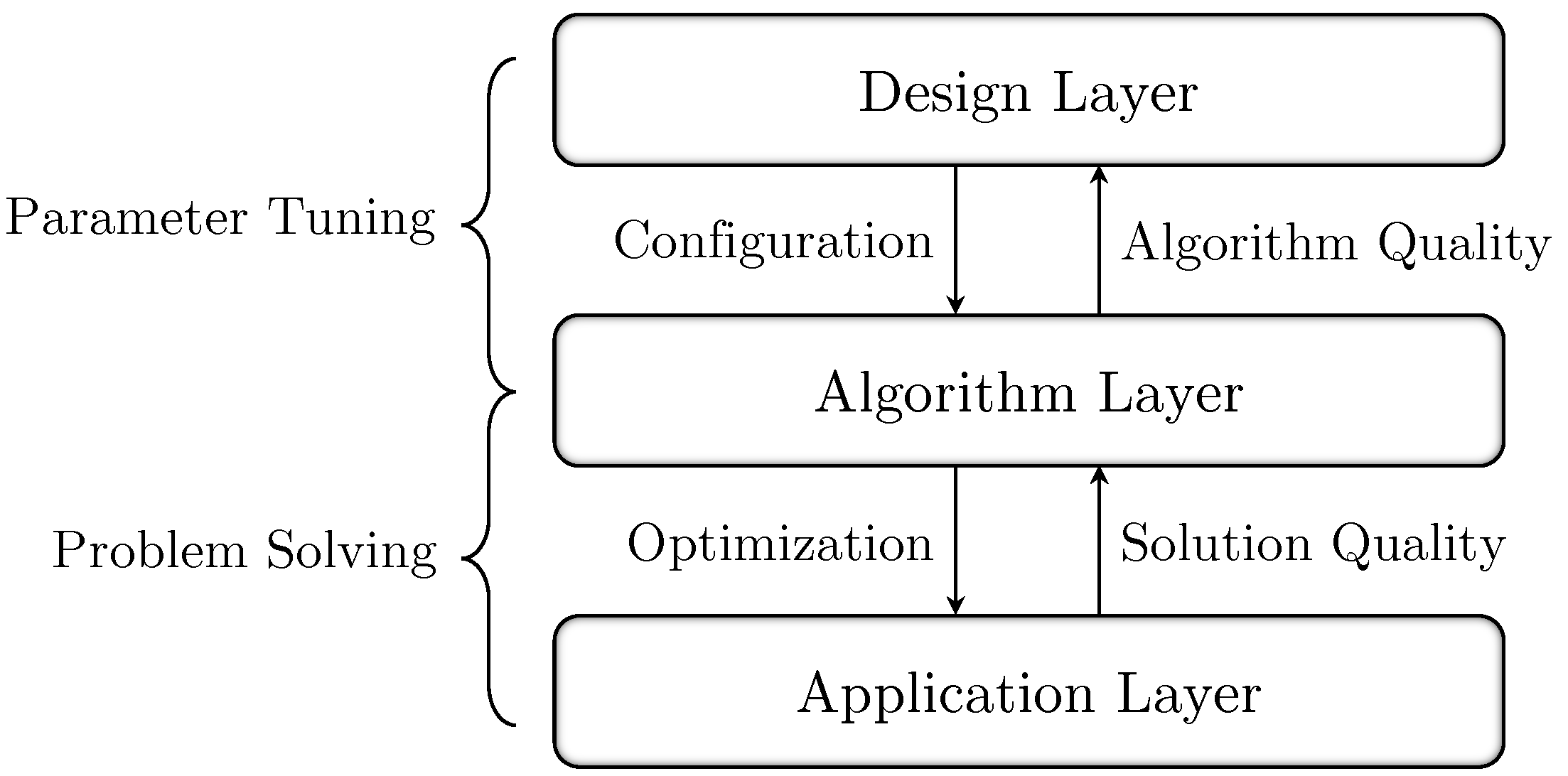
3.2. Parameter Tuning Problem

The choice of parameters for algorithms is essential for their effectiveness and efficiency. The determination of suitable parameters for algorithms can be approached using the parameter tuning (or parameter configuration) problem [2]. The parameter tuning problem can be specified according to Eiben and Smit [7].

As Figure 1 demonstrates, different layers of the problem structure are considered and these are connected with a control and an information flow. The application layer describes the given optimization problem (here, the MDPDPTWHV, as in Section 3.1), which is solved by an algorithm (algorithm layer, here, e.g., the GGA from Section 4.1). How this particular algorithm is designed with respect to parameter configuration is described in the design layer. The quality of the parameter configuration chosen for an algorithm is evaluated in terms of solution quality.

Figure 1. Control flow (left) and information flow (right) through the different layers in parameter tuning [7].

The PTP arises, among others, in the optimization of parameter settings for meta-heuristics [2]. Thus, many optimization methods such as a Genetic Algorithm depend on various known parameters that can be optimally chosen so that their performance can be improved in terms of finding good solutions [4]. Obviously, the performance of a meta-heuristic depends on the configuration of its parameters. Nevertheless, the configuration problem has not been formally considered in scientific publications for a long time [39]. The authors of ref. [40] describe how, until around 1999, parameter selection in the development of meta-heuristics was carried out manually. After evaluating various configurations, the one that delivered the best result was selected. The selection was thus often made on the basis of expert knowledge about the respective optimization problem. However, according to the No Free Lunch Theorem, there is no universal algorithm whose computations have the same solution quality for all optimization problems [34], so parameter tuning is by no means a one-time problem and it definitely makes sense to automate it [2].

It is worth pointing out that, besides the static parameter configuration, there are also dynamic, adaptive or self-adaptive approaches (cf. [8]). For these techniques, Machine Learning (ML) approaches are often reasonably applied due to their promising results. An overview of which meta-heuristic-related configuration problems can arise, and how ML techniques are applied to solve them for algorithms solving combinatorial optimization problems, can be found in [41]. A review of such learn-heuristics, especially for routing problems, is given by [42], while, in [43], a literature review for adaptive parameter configuration for evolutionary algorithms is given.

4. Proposed Methods

The methods to solve the considered problems, the MDPDPTWHV and the Parameter Tuning Problem, are presented in this section. In Section 4.1, a detailed overview of the Grouping Genetic Algorithm is given, followed by a comprehensive description of the Bayesian Optimization approach in Section 4.2.

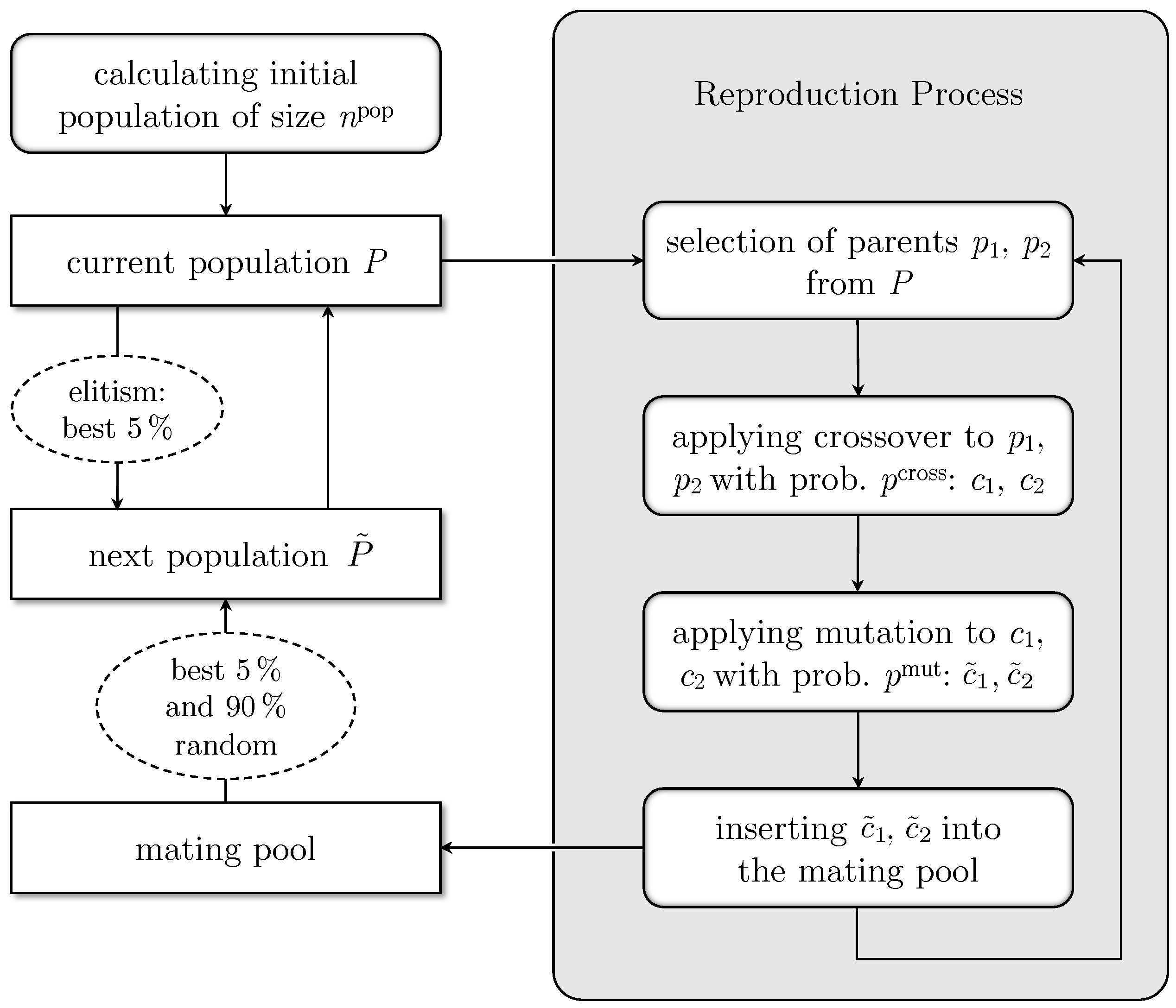
4.1. Grouping Genetic Algorithm Framework

Genetic algorithms go back to [44]. They iteratively apply certain operators to a population of solutions so that, on average, each new generation tends to be better than the previous one, according to a predefined fitness criterion. The fitness criterion measures the ability of an individual to survive in a population and the algorithm strives to maximize fitness. The stop criterion is usually specified as a fixed number of generations or as a time limit for execution. In the end, the best solution found is returned. Genetic algorithms generally provide good results for complex routing problems (see, e.g., [14,21]), so it makes sense to focus on these.

In particular, the Grouping Genetic Algorithm presented in [1] produces adequate results for the MDPDPTWHV. Here, the authors show that the considered GA variants with population management regarding general replacement with elitism promise a good solution quality for the presented problem. However, the complexities of the problem instance’s data structure can be various. Hence, in this paper, the GGA is extended by new mutation and repair operators in order to investigate which combination of operators is suitable for a given data structure. The GGA’s general replacement version with binary tournament selection is used. In addition, the GGA of [1] has been enhanced through the permission of infeasible solutions by which the entire search space is investigated more effectively. An overview of the procedure of the GGA is given in Figure 2. For all terms and concepts of Genetic Algorithms, we kindly refer readers to [45].

Figure 2. Grouping Genetic Algorithm framework with population management: general replacement with elitism.

The procedure of the GGA can be explained as follows: at the beginning, a population P of $n^{\mathrm{pop}}$ individuals is determined. It is assumed that each individual has a fitness value. This is equal to the sum of the variable and fixed costs of the vehicle routing solution (see objective function (1)) and also integrates a penalty term for non-served requests. The fitness value is to be minimized in the proposed GA variant and can be written as follows:

$$\begin{array}{c}\hfill \sum _{i,j\in \mathcal{V}}{c}_{ij}{x}_{ij}+\sum _{d\in {\mathcal{D}}_s}\sum _{j\in {\mathcal{N}}_p}{f}_d{x}_{dj}+\gamma \sum _{i\in {\mathcal{N}}_p}\left(1-\sum _{j\in \mathcal{N}}{x}_{ij}\right).\end{array}$$

(26)

In general, for the penalty term in (26), the weight $\gamma$ is to be chosen in such a way that the consideration of non-served requests results in the worst possiblesolution [46]. In order to achieve this constraint, $\gamma$ is empirically chosen as follows:

$$\begin{array}{c}\hfill \gamma ≔2·\underset{i,j\in \mathcal{V}}{max}\{c_{ij}+c_{ji}\}+\underset{d\in \mathcal{D}}{max}\left\{f_d\right\}.\end{array}$$

(27)

Please note that, if the GGA is implemented in a variant that only allows feasible solutions according serving all requests in an instance, $\gamma$ in (27) has to be set to $\gamma ≔0$. However, in preliminary studies, it has been found out that, the MDPDPTWHV allowing infeasible solutions in the manner of unserved requests, together with the fitness function (26) and penalty term (27), leads to an improved solution quality of the GGA.

Each individual is computed by using several sequential double-insertion heuristics that create routes one after another by inserting customers at their best possible position. To enhance the diversity of the initial population, 25% of the individuals are generated with Best Insertion, which starts the route with one request and inserts the best corresponding request in each iteration; 50% with Random Insertion, which chooses a random request for insertion in every iteration (cf. [1]); and 25% with a Regret-k heuristic (cf. [16]), which calculates a regret value to evaluate how much a greedy insertion will cost in the end and selects the request that has the highest costs (see Equation (30) in Section 4.1.5). A high level of diversity is achieved, as no duplicates are allowed within the population. The percentage values for applying the insertion heuristics considered have been determined in preliminary studies (cf. [1]).

As long as the maximum number of generations ${\gamma }^{max}$ has not been met, two parents $p_1,p_2$ for generating offsprings are selected (cf. Section 4.1.2). With a probability of $p^{\mathrm{cross}}$, one crossover operator variant is applied to $p_1$ and $p_2$, as in [1], in order to create two children $c_1$ and $c_2$ (cf. Section 4.1.3). Moreover, each child is modified by using one of the mutation operators with probability $p^{\mathrm{mut}}$ and so two mutated children ${\tilde{c}}_1$ and ${\tilde{c}}_2$ are generated (see Section 4.1.4). In case no operator is applied, the created offsprings are just clones of their ancestors. Generated individuals are stored in a mating pool from which the next population is selected. Finally, the best individual regarding its fitness is returned. Please note that $n^{\mathrm{pop}},{\gamma }^{max},p^{\mathrm{cross}}$, and $p^{\mathrm{mut}}$ are parameters that are set manually. These parameters have have been determined in preliminary tests (cf. [1]).

The most difficult part of a GA is to find a good solution representation or genotype encoding, respectively, so that the crossover and mutation operators do not have to be too complex and decoding from genotype to phenotype is not time-consuming. For this reason, the approach of [1] is implemented as a Grouping GA in which each vehicle is represented by a gene and the pickup and delivery customers are grouped with their request index. A genotype encoding then stores the assignment of a request to the executing vehicle and can be represented by a vector of integers.

Figure 3 shows that the vehicles are represented by negative index values. All subsequent positive integers indicate the requests served by the corresponding vehicle. This encoding implies that a route for each vehicle (e.g., route 2 in Figure 3) has to be calculated, whenever the genotype decoding is necessary, e.g., for the determination of the fitness value. Since this is very time-consuming and not necessarily deterministic with regard to the applied heuristics, the corresponding phenotype of an individual is also be stored (cf. [1]), i.e., the vehicle routing solution. Thus, it is less likely that good features of an individual are removed from the phenotype when applying crossover or mutation operators. Please note that the phenotype must always be modified together with the genotype during the solution process.

Figure 3. Genotype encoding for the Grouping Genetic Algorithm.

The following Section 4.1.1, Section 4.1.2, Section 4.1.3, Section 4.1.4 and Section 4.1.5 describe in detail the operators extended compared to [1] and those whose control parameters are to be optimized, i.e., mutation and repair operators. The selection and crossover operators, as well as population management, are adopted from the GGA of [1].

4.1.1. Population Management

Due to the promising results of the GGA with general replacement as population management [1], this variant was implemented in the present framework. Hence, a mating pool of 1.5 times the generation size is filled with children, whereas duplicates are prevented. In order to keep the best solutions from the last generation, elitism is applied by copying the best 5% of the generation into the next. Subsequently, the best 5% of individuals from the mating pool are selected and the rest of the next generation is randomly filled with individuals from the mating pool (cf. Figure 2).

4.1.2. Selection

In order to select parents without duplicates for offspring generation, binary tournament is used, since this selection approach has provided the most promising results. Here, two individuals, called a tournament, are chosen randomly from the population and the best individual is used as the first parent. The second parent is selected analogously.

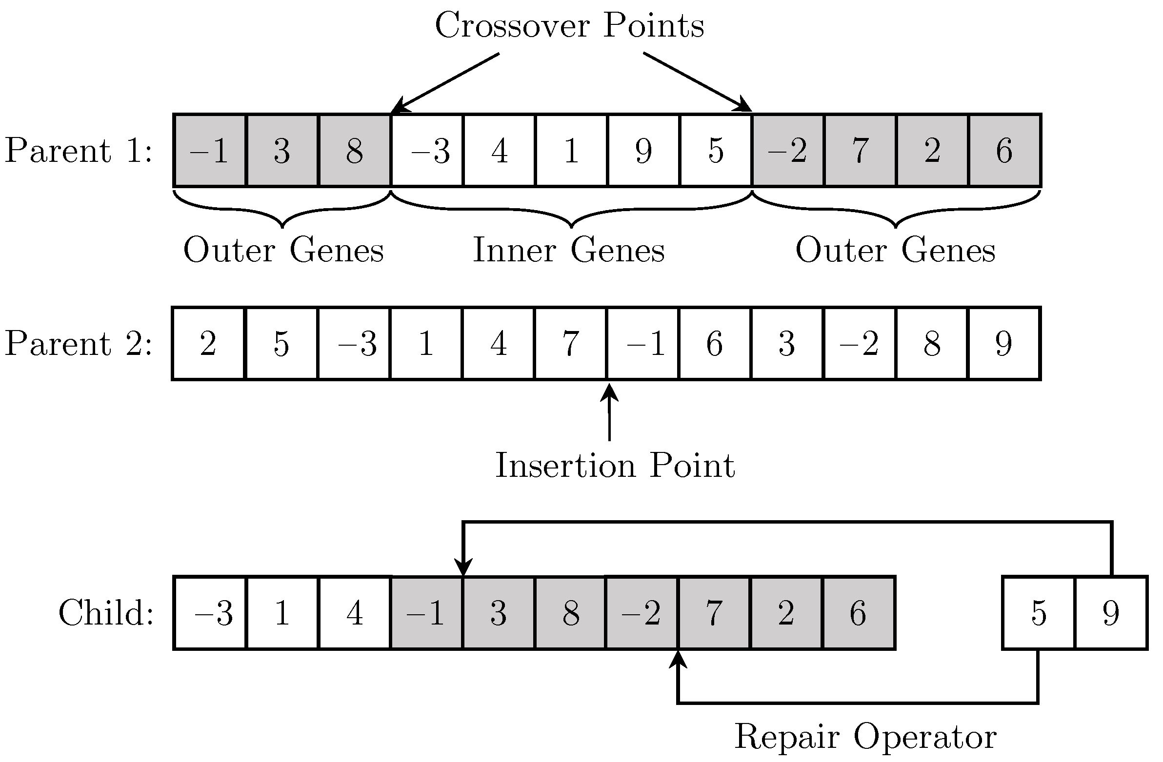
4.1.3. Crossover Operator

The implemented group-oriented crossover variants are adopted from the GGA of [1]. A simplified illustration of how the crossover works for a representation with nine requests distributed over three possible vehicles is given in Figure 4. Two crossover points (both of them between two genes) are randomly chosen for parent 1. Then, all genes between the two crossover points (inner genes) are transferred with a probability of 50% and, otherwise, the genes outside of them (outer genes) are chosen at a randomly chosen insertion point into parent 2 to generate a child. This requires double-served requests and double-used vehicles coming from parent 2 to be deleted from the child. In doing so, non-served requests have to be re-inserted into the child by repair operators (see Section 4.1.5). In Figure 4, the inner genes are not transferred into the child. The outer genes mean that vehicles 1 and 2 have to be eliminated from the child. In addition, requests 2 and 7 must be removed. Finally, requests 5 and 9 remain and have to be re-inserted by a repair operator again. For a detailed explanation, we kindly refer readers to [1].

Figure 4. Crossover operator when transferring genes from parent 1 to parent 2.

4.1.4. Mutation Operators

Contrary to [1], the mutation operators are basically classified in vehicle-based and request-based mutations. The selection of the operator class is carried out by a specific probability value $p^{\mathrm{choice}}\left(n\right)$ that models the likelihood for choosing request-based mutation in generation n:

$$\begin{array}{c}\hfill p^{\mathrm{choice}}\left(n\right)=0.1·exp\left(ln\left(8\right)\frac{n}{{\gamma }^{max}}\right).\end{array}$$

(28)

In this way, the value $p^{\mathrm{choice}}$ of Equation (28) prefers vehicle-based operators in the beginning of the Genetic Algorithm and request-based operators at the end (the value $p^{\mathrm{choice}}$ starts at 0.1 in the first generation, $n=0$, and ends at 0.8 in the last generation, $n={\gamma }^{max}$). In this manner, the trade-off is controlled between solution quality and computational time, since the vehicle-based mutation has a faster and broader investigation in the search space, while request-based mutation has a slower and more accurate search behaviour, which, in general, describes exploration vs. exploitation. Please note that, due to the choice of probability $p^{\mathrm{choice}}$, vehicle-based and request-based mutation are not equally weighted.

The vehicle-based mutation is executed through selecting a vehicle index. The corresponding vehicle is deleted from the genotype and phenotype. Afterwards, all requests served by the erased vehicle must be reinserted, which is carried out by a repair operator (see Section 4.1.5), such that the solution holds all constraints. Here, a new vehicle may also have to be introduced. A simplified scheme of the mutation operator is given at the top of Figure 5. As in [1], the following four vehicle selection mechanisms are applied in order to tackle the problem of heterogeneity:

Figure 5. Mutation operators and mutated child to be repaired (using an additional empty vehicle if needed) with vehicle-based mutation (top) and request-based mutation (bottom).

• Costs/Number-of-Request Ratio. The ratio of route costs and the number of served requests is calculated for each vehicle and used to generate a roulette wheel. By spinning the roulette wheel, a vehicle index is selected. In particular, expensive routes with a small number of requests are preferred for removal.
• Number of Requests. The vehicle with the minimum number of requests is used for deletion.
• Random Vehicle Index. Here, a random vehicle index is selected, thus all vehicles are equally likely to be chosen.
• Random Genotype Position. The variant chooses a random position within the genotype and selects the respective vehicle index. Hence, vehicles with many requests are preferred.

Request-based mutation is a newly added concept. Particularly if instances have many requests per vehicle or if in the course of the search the solution space must be examined more precisely for intensification, it is useful to remove individual requests from the genotype or phenotype, respectively. Basically, a number of requests to be released is randomly determined and then eliminated from the individual with one of the mechanisms described below. A simplified procedure is shown at the bottom of Figure 5.

• Historical Request Pair. This concept is adopted from the approach of [17] and uses a matrix ${\left(h_{ij}\right)}_{i,j\in \mathcal{R}}$ of weights for all requests $\mathcal{R}$. The matrix stores how promising a combination of two requests on the same vehicle is. To do so, the elite is evaluated after each generation and a matrix element $h_{ij}$ is increased by one if the requests i and j are served together on one vehicle. The matrix ${\left(h_{ij}\right)}_{i,j\in \mathcal{R}}$ can be interpreted as long-term memory. Since combinations with high quality in a certain generation do not necessarily have to be globally optimal, the matrix is adjusted during each generation through reducing $h_{ij}$ by a factor $\tau \in (0,1)$, i.e., $h_{ij}≔\tau h_{ij}$. To determine the requests to be eliminated, a score ${\sigma }_i$ is specified in which $h_{ij}$ values are summed up if request j is served with i on the same vehicle in the considered individual. Requests with low ${\sigma }_i$ are non-promising combinations on the same vehicle and, consequently, are removed from the individual.
• Similarity Measure. The variant is derived from the similarity-measure-based removal operator of [16]. Here, the first request is chosen randomly and, additionally, those requests are removed which are similar with respect to the measure ${\tilde{\rho }}_{ij}$ from Equation (29), i.e., those that have the smallest values. Please note that $i,j\in \mathcal{R}$ and request i have pickup customer i and delivery customer $i+n$ (see Section 3.1).

  $$\begin{array}{cc}\hfill {\tilde{\rho }}_{ij}=& {\alpha }_1(c_{ij}+c_{i+n,j+n})+{\alpha }_2\left(\right|a_i-a_j|+|a_{i+n}-a_{j+n}\left|\right)\hfill \\ \hfill & +{\alpha }_3\left(\right|b_i-b_j|+|b_{i+n}-b_{j+n}\left|\right)+{\alpha }_4\left(\right|p_i-p_j\left|\right)\hfill \end{array}$$

  (29)

Thus, those requests are defined as similar whose pickup and delivery nodes, start and end time windows, and demands to be transported are close to each other, since, for these, the exchange to another vehicle offers potential for direct insertion and, therefore, an improvement in the fitness value. For comparability, all values are scaled to the interval $[0,1]$. The weights ${\alpha }_k,k=1,\dots ,4$ are elements of ${\mathbb{R}}^{\ge 0}$.

Additionally, a so-called swap operator with a probability of 20% is applied, after one of the six mutation variants is taken into account. This operator tries to swap used and free vehicles to minimize the sum of fixed costs. In order to keep the search in the solution space broad, the choice of vehicles to be swapped is guided by a roulette wheel.

4.1.5. Repair Operator

When applying crossover or mutation operators, the individual has often to be repaired due to removed requests. During repair, requests need to be re-inserted. Here, several insertion methods are used that determine the best insertion positions for each request with respect to a cost value. Contrary to [1], a Regret-k insertion method beside the greedy insertion is implemented. The approaches are quite similar to the double insertion heuristics used for generating the initial population. However, the proposed repair operators are parallel insertion heuristics, i.e., the possible insertion positions are evaluated for all available vehicles. If there are requests that cannot be served by available vehicles, a new (empty) vehicle has to be introduced whenever feasible.

• Greedy Insertion. For each request, the insertion costs for all possible positions in each vehicle are calculated and the position with the lowest costs is chosen (cf. [1]).
• Regret-$\mathbf{k}$ Insertion. For each request r, the difference in how much worse it is to insert a request in the k-th best vehicle $v_k$ instead of the best one $v_1$ is calculated, while the differences from the best to the k-th best vehicle are summed up. The request $\tilde{r}$ with the maximum value is supposed to be inserted into its best position in the current iteration, since, later on, the insertion costs increase (cf. [16]). Formally, this can be written as in (30):

  $$\begin{array}{c}\hfill \tilde{r}=arg\underset{r}{max}\left\{\sum _{l=1}^k({\mathsf{\Delta }}_r^{v_l}-{\mathsf{\Delta }}_r^{v_1})\right\}.\end{array}$$

  (30)

The Regret-k insertion is applied for $k=2,3,4,\delta$. Additionally, in order to avoid repeated solutions from one individual to another, a tabu list can be applied which includes the vehicle in which a request should preferably not be inserted again.

Both the two new request-based mutation variants, as well as the Regret-k repair operator (with possible tabu list), effect the GGA in the manner that the exploration of a known area in the solution space will be improved. This is very important in the context of the MDPDPTWHV in comparison to related, less complex vehicle routing problems, since, with higher problem complexity, the challenge of finding a sufficiently good solution with only simple operators intensifies. Hence, the rough searching intended by deleting an entire vehicle leads, rather, to new areas than does investigating a complex smaller part of the solution space.

4.2. Bayesian Optimization for Tuning the Parameters of the Grouping Genetic Algorithm

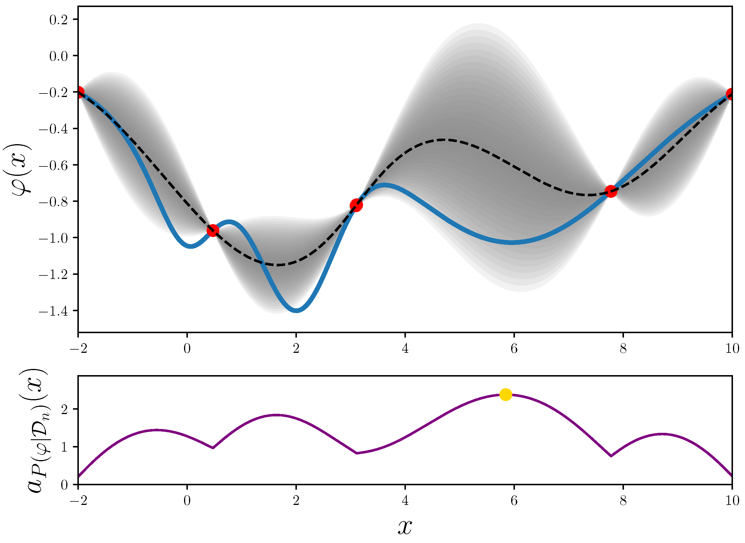
As depicted in Figure 1, the Parameter Tuning Problem is the optimization problem which is embedded in the top layer above the solution approach for solving the origin problem. Due to this fact, the considered origin problem’s solution algorithm has to be executed reasonably often, according to the PTP, in order to find a sufficient algorithm parameter configuration (see Section 3.2). Hence, a common drawback of many parameter tuning approaches for meta-heuristics (see, e.g., the methods in Section 2) is the considerable number of evaluations of the objective function required to determine the best parameter configuration [28].

As the performance of a Genetic Algorithm is sensitive to the parameter setting and the structure of a problem instance, the evaluation of specific parameter configurations can be very time-consuming. Moreover, optimizing the parameters of meta-heuristics is a black box problem, since the relationship between the parameter configurations of the algorithm and its performance cannot be measured metrically [2].

Altogether, Bayesian Optimization is a reasonable choice as a parameter tuning algorithm, since this method manages to cope with few evaluations of the objective function to be optimized, which also need not be known [28,47]. Furthermore, BO is well applicable to functions defined in a solution space with dimension $D\le 20$ (number of parameters) and tolerates noise with respect to the function evaluation [48], which is typical behaviour for stochastic methods like a GA. Last but not least, the results of [28] show that BO is, in general, a good approach in solving the Parameter Tuning Problem for EAs. For a detailed overview of Bayesian Optimization, we kindly refer readers to [47,48,49].

Let $\phi :\mathbb{X}\to \mathbb{R}$ be an unknown black box function that cannot be modeled in closed form, i.e., for an argument $\mathit{x}\in \mathbb{X}\subseteq {\mathbb{R}}^D$, the function value $\phi \left(\mathit{x}\right)$ can only be determined by evaluating $\phi$. In the Parameter Configuration Problem, $\phi$ describes the utility of a parameter vector $\mathit{x}\in \mathbb{X}$, which can be, e.g., the mean of the objective values over all the considered instances. The goal of Bayesian Optimization is to find a configuration ${\mathit{x}}^{\ast }=arg{min}_{\mathit{x}\in \mathbb{X}}\phi \left(\mathit{x}\right)$ describing the global minimum of $\phi$. The method iteratively learns a probabilistic model that estimates the utility function $\phi$ by known function values $\phi \left(\mathit{x}\right)$ of different points $\mathit{x}\in \mathbb{X}$ in the parameter space. For this purpose, an a priori probability distribution $P\left(\phi \right)$ over the utility function $\phi$ and an acquisition function $a_{P\left(\phi \right)}:\mathbb{X}\to \mathbb{R}$, that quantifies the utility of evaluating the function $\phi$ at each parameter configuration $\mathit{x}$, are required [50]. Let n data points in the set ${\mathcal{D}}_n={({\mathit{x}}_i,y_i)}_{i=1,\dots ,n}$ with $y_i=\phi \left({\mathit{x}}_i\right)+{\epsilon }_i$ be known for function $\phi$. Then, Bayesian Optimization iteratively repeats the following three steps [47]:

• Find the next configuration ${\mathit{x}}_{n+1}$ whose evaluation is most promising, i.e., which maximizes the acquisition function under the condition of the known data points ${\mathcal{D}}_n$:

  $${\mathit{x}}_{n+1}=arg\underset{\mathit{x}\in \mathbb{X}}{max}{a}_{P(\phi \mid {\mathcal{D}}_n)}\left(\mathit{x}\right).$$
• Determine $y_{n+1}=\phi \left({\mathit{x}}_{n+1}\right)+{\epsilon }_{n+1}$ with possible noise ${\epsilon }_{n+1}$ and add $({\mathit{x}}_{n+1},y_{n+1})$ to the previous data points: ${\mathcal{D}}_{n+1}={\mathcal{D}}_n\cup \left\{({\mathit{x}}_{n+1},y_{n+1})\right\}$.
• Update the probability model $P(\phi \mid {\mathcal{D}}_{n+1})$ and, consequently, the acquisition function $a_{P(\phi \mid {\mathcal{D}}_{n+1})}$.

Here, the update of the probabilistic model is carried out in step (3) via the Bayes’ Theorem (31), where

$$\begin{array}{c}\hfill P(\phi \mid {\mathcal{D}}_{n+1})\propto P({\mathcal{D}}_{n+1}\mid \phi )P\left(\phi \right).\end{array}$$

(31)

The theorem states that the posteriori probability distribution $P(\phi \mid {\mathcal{D}}_{n+1})$ for the new data points ${\mathcal{D}}_{n+1}$ is proportional to the a priori model $P\left(\phi \right)$ multiplied by the similarity of the data points ${\mathcal{D}}_{n+1}$ to the assumed model for $\phi$.

In condition (31), $P({\mathcal{D}}_{n+1}\mid \phi )$ consequently expresses how likely the data are under the model assumptions that are known a priori. If the assumption is that the utility function $\phi$ is very smooth and noise-free, data with high variance should be recognized as less likely than data that hardly deviate from the mean [47].

Figure 6 shows an iteration of Bayesian Optimization. The black box function $\phi \left(x\right)$ to be optimized is drawn here in blue and the mean estimated function $m\left(x\right)$ is dashed in black. At each point $x\in \mathbb{X}$ the estimated utility function value $m\left(x\right)$ with a variance of $k(x,x)$, which is described by the confidence interval in y-direction (gray), can be determined depending on the already evaluated data points ${\mathcal{D}}_n$ (red) and the used a priori model $P\left(\phi \right)$. These data are incorporated into the acquisition function (shown below), which determines a score for evaluating the possible x vectors. Here, the selected value $x_{n+1}$ receives a high score because the knowledge about the range containing $x_{n+1}$ is not yet enough for a sufficiently good estimation, as the variance is high.

Figure 6. Bayesian Optimization with Gaussian Processes as a priori model (top) and acquisition function $a_{P(\phi \mid {\mathcal{D}}_n)}$ (bottom).

The solution quality of Bayesian Optimization significantly depends on the choice of the a priori probability distribution (see Section 4.2.1) and on the evaluation of the utility by a surrogate model, i.e., the acquisition function (see Section 4.2.2). Both components are described in the following subsections.

4.2.1. Gaussian Processes

For a priori distributions, possible models are Gaussian Processes, Random Forests or Bayesian Neural Networks [50]. Gaussian Processes are most commonly chosen in the literature [48] and also provide promising results in [28,35,50]. Therefore, a Gaussian Process (GP) is used in the presented Bayesian Optimization approach. In the following, some insights into the GP used here are given. For a detailed description of Gaussian Processes, we kindly refer readers to [51,52].

For a Gaussian Process, a covariance function (also called a kernel) has to be defined. It can be assumed that the utility function $\phi$ for the problem at hand is non-smooth (cf. Section 4.1). This is because different function values $\phi \left(\mathit{x}\right)$ can be obtained due to the uniform distributed randomly chosen operators, even if $\phi$ is evaluated several times with the same parameters $\mathit{x}$. Thus, kernel functions coming from the class of Automatic Relevance Determination (ARD) Matérn kernels are appropriate for the Parameter Tuning Problem presented, since they can model non-smooth functions [53]. In the BO approach used in this paper, the ARD Matérn $\frac{5}{2}$ kernel is applied, which is defined as follows:

$$\begin{array}{c}\hfill k_{\mathrm{M}52}(\mathit{x},{\mathit{x}}^{\prime })={\theta }_0\left(1+\sqrt{z}+\frac{z}{3}\right)exp\left(-\sqrt{z}\right)\end{array}$$

(32)

with $z=5r^2(\mathit{x},{\mathit{x}}^{\prime })$, while the function $r^2$ is defined as $r^2(\mathit{x},{\mathit{x}}^{\prime })={\sum }_{d=1}^D\frac{{(x_d-x_d^{\prime })}^2}{{\theta }_d^2}$. Since the influence of the individual parameters on the solution quality is not known a priori, the parameter ${\theta }_d=1$ is set for all $d=0,\dots ,D$ within $r^2(\mathit{x},{\mathit{x}}^{\prime })$ in the presented approach.

Due to the stochastic nature of the GGA to be optimized, the solution for a given parameter configuration is expected to be subject to noise [2]. To model this noise, the kernel function (33) is additionally used [51]:

$$\begin{array}{c}\hfill k_{\mathrm{Noise}}(\mathit{x},{\mathit{x}}^{\prime })=\left\{\begin{array}{cc}{\sigma }_n^2\hfill & ,\mathit{x}={\mathit{x}}^{\prime }\hfill \\ 0\hfill & ,\mathrm{sonst}\hfill \end{array}\right..\end{array}$$

(33)

The parameter ${\sigma }_n^2$ describes the variance of the modeled noise. Altogether, the covariance function $k(\mathit{x},{\mathit{x}}^{\prime })$ (34), considered for the Gaussian Process in the BO approach at hand, is composed of (32) and (33) (cf. defining GP kernels in [51]):

$$\begin{array}{cc}\hfill k(\mathit{x},{\mathit{x}}^{\prime })& =k_{\mathrm{M}52}(\mathit{x},{\mathit{x}}^{\prime })+k_{\mathrm{Noise}}(\mathit{x},{\mathit{x}}^{\prime }).\hfill \end{array}$$

(34)

In order to purposefully design the choice of the next parameter configuration to be evaluated in step (1), a reasonable acquisition function must be defined. This function makes use of the model assumed by the Gaussian Process to predict the utility for evaluating certain parameter settings $\mathit{x}\in \mathbb{X}$.

4.2.2. Acquisition Function

The acquisition function $a_{P\left(\phi \right)}$ is designed to estimate, based on the current data ${\mathcal{D}}_n$, which areas of the parameter space $\mathbb{X}$ to investigate in order to improve the model’s prediction of the Gaussian Process. Therefore, the acquisition function should be constructed to achieve a high value at parameters $\mathit{x}\in \mathbb{X}$, where the predicted utility function value $\phi \left(\mathit{x}\right)$ is low or the prediction’s quality is poor, i.e., there is too little information available on that part of the considered parameter space for a sufficiently accurate estimation [47]. These two cases describe the classical problem of exploitation vs. exploration. This is tackled in several acquisition functions that can be found in the literature, such as Probability of Improvement, GP Upper Confidence Bound, and Expected Improvement (EI) [53]. Since EI automatically controls the balance between exploitation and exploration, and achieves sufficiently good results in BO approaches [28], it is also used in the approach at hand. With respect to the currently observed data ${\mathcal{D}}_n$, the acquisition function with EI is defined as follows:

$$\begin{array}{c}\hfill a_{P(\phi \mid {\mathcal{D}}_n)}^{\mathrm{EI}}\left(\mathit{x}\right)=(\phi \left({\mathit{x}}^{\ast }\right)-m\left(\mathit{x}\right))\mathsf{\Phi }\left(z\right)+\sigma \left(\mathit{x}\right)\varphi \left(z\right)\end{array}$$

(35)

with $z=\frac{\phi \left({\mathit{x}}^{\ast }\right)-m\left(\mathit{x}\right)-\xi }{\sigma \left(\mathit{x}\right)}$, where ${\mathit{x}}^{\ast }$ is the best parameter configuration so far, i.e., ${\mathit{x}}^{\ast }=arg{min}_{\mathit{x}\in {\mathcal{D}}_n}\phi \left(\mathit{x}\right)$, and ${\sigma }^2\left(\mathit{x}\right)$ describes the predicted variance $k(\mathit{x},\mathit{x})$. The function $\varphi$ represents the density function and $\mathsf{\Phi }$ the cumulative distribution function of the normal distribution $\mathcal{N}\left(m\right(\mathit{x}),k(\mathit{x},\mathit{x}\left)\right)$. By the acquisition function $a_{P(\phi \mid {\mathcal{D}}_n)}^{\mathrm{EI}}$ in (35), $\mathit{x}\in \mathbb{X}$ are preferred if $m\left(\mathit{x}\right)<\phi \left({\mathit{x}}^{\ast }\right)$, i.e., $\mathit{x}$ could reduce the utility function value, or if there is a high variance ${\sigma }^2\left(\mathit{x}\right)$, i.e., the utility function value for $\mathit{x}$ cannot be estimated with sufficient quality based on the current data ${\mathcal{D}}_n$. To influence exploitation and exploration in addition to the intrinsic control by the two summands of (35), a parameter $\xi \ge 0$ can be selected. The larger $\xi$ is, the more exploration is preferred. Therefore, it is recommended to start with a sufficiently large $\xi$ and to let it approach zero over the Bayesian Optimization process [47].

To approximate the best parameter configuration determined by the acquisition function ${\mathit{x}}_{n+1}=arg{max}_{\mathit{x}\in \mathbb{X}}{a}_{P(\phi \mid {\mathcal{D}}_n)}^{\mathrm{EI}}\left(\mathit{x}\right)$, which has to be evaluated next for $\phi$, $a_{P(\phi \mid {\mathcal{D}}_n)}^{\mathrm{EI}}$, is evaluated on a sufficiently large number of random parameter configurations $\mathit{x}\in \mathbb{X}$. The best configuration is chosen as ${\mathit{x}}_{n+1}$.

5. Results and Discussion

In this section, the results of the Bayesian Optimization approach regarding the parameter configuration for the Grouping Genetic Algorithm are presented. In doing so, the most promising GGA variant of [1] (described in Section 4.1) is compared to a state-of-the-art algorithm developed to solve a related Pickup and Delivery Problem, the Adaptive Large Neighbourhood Search (ALNS) from [16]. In addition, an approach which randomly selects several parameter configurations and chooses the parameters with best fitness values of the GGA is applied in order to show that the BO performs the optimization of the parameter configuration in a goal-oriented manner.

Please note that the parameter configuration of the ALNS has not been optimized by the Bayesian Optimization approach, since the GGA, with its initial and optimized parameter configuration, is supposed to be compared to a state-of-the-art algorithm regarding the considered Pickup and Delivery Problem. Moreover, the ALNS does not offer the feature to tune the parameter configuration used, since it adjusts the parameters adaptively during the optimization process (cf. [16]).

At first, we describe how the benchmark data sets are created (see Section 5.1). Then, the results for the initial and parameter optimized GGA compared to the ALNS are presented (see Section 5.2). Finally, the different parameter configurations, as well as improvements in each problem class, are highlighted (see Section 5.3).

5.1. Data Generation

The evaluation of the meta-heuristics is performed using self-generated problem instances. These were created with a single-depot data set generator and on the basis of practical circumstances and experience (cf. [1]), so that several practically oriented single-depot problem instances with different depot positions are built and layered on top of one another for the generation of multi-depot instances. In this way, data sets with 1200 instances each, and 1, 4, 6, 8, and 9 depots, are constructed. According to our cooperation partner, these data sets represent the structures in reality. Each of the data sets contains 12 problem classes including 100 instances created with the same parameters in the data set generator. Thus, 60 classes with different characteristics regarding, e.g., number of depots, time window size, vehicle capacity or the constellation of the customer positions, are provided [1]. All data sets are available in [54].

5.2. Parameter Configuration

The initial parameters used for the GGA have been determined in preliminary studies during the development of the solution approach. They are displayed in Table 2.

Table 2. Initial parameters for evaluating the GGA variants.

Param.	Value	Description
$n^{\mathrm{pop}}$	50	population size
$p^{\mathrm{cross}}$	1.0	crossover rate
$p^{\mathrm{mut}}$	0.3	mutation rate
${\gamma }^{max}$	250	maximum number of generations
$\omega$	1.5	relative mating pool size with respect to population size (i.e., $n^{\mathrm{pop}}=50$ results in 75 individuals)
$\lambda$	0.05	proportion of the elite within the population
$p_i^{\mathrm{cross}}$	0.5	probability of applying one of the crossover variants, $i=1,2$
$p_1^{{\mathrm{mut}}_v}$	0.4	probability of applying vehicle-based mutation Costs/Number-of-Request Ratio
$p_2^{{\mathrm{mut}}_v}$	0.4	probability of applying vehicle-based mutation Number of Requests
$p_3^{{\mathrm{mut}}_v}$	0.1	probability of applying vehicle-based mutation Random Vehicle Index
$p_4^{{\mathrm{mut}}_v}$	0.1	probability of applying vehicle-based mutation Random Genotype Position
$p_1^{{\mathrm{mut}}_r}$	0.6	probability of applying request-based mutation Historical Request Pair
$p_2^{{\mathrm{mut}}_r}$	0.4	probability of applying request-based mutation Similarity Measure Selection
$p_1^{\mathrm{repair}}$	0.55	probability for using the Greedy Insertion Repair Operator
$p_2^{\mathrm{repair}}$	0.25	probability for using the Regret-2 Repair Operator
$p_3^{\mathrm{repair}}$	0.10	probability for using the Regret-3 Repair Operator
$p_4^{\mathrm{repair}}$	0.05	probability for using the Regret-4 Repair Operator
$p_5^{\mathrm{repair}}$	0.05	probability for using the Regret-$\delta$ Repair Operator

For optimizing the parameters (see Table 2), the Bayesian Optimization is applied on the probabilities for mutation and repair operators, since tuning parameters such as $n^{\mathrm{pop}},{\gamma }^{max},\omega$, and $\lambda$ particularly affect the number of individuals to be generated. Therefore, previous investigations have shown that optimizing these parameters results in the intuitive solution of setting these values to their maximum. Furthermore, the choice for crossover and mutation rates is reasonable with respect to the problem at hand. Finally, due to the similarity of the crossover operators, optimizing the selection probabilities of these variants will not have a huge impact on the solution quality.

In order to determine the best configuration of parameters to be optimized, the BO is performed with 20 iterations. Beforehand, for modeling a sufficiently good a priori probability distribution, the utility function values are determined for 10 randomly drawn parameter combinations. In this way, the Bayesian Optimization is applied to 10 randomly chosen problem instances (i.e., the training data) from each class to identify parameters with which the GGA has the best solution quality regarding the mean of the objective value over these instances. Since the GGA is a stochastic meta-heuristic, each instance is additionally evaluated five times to obtain a stable parameter configuration. In preliminary studies, it was established that a larger set of training data yields worse GGA results, as well as an increased computational time for the BO approach. Hence, the number of instances used for training data is chosen with respect to efficiency. Since the selection of training instance data sets is also a combinatorial optimization problem, it is evident that the manual tests for finding the best training sets represent a limitation in this study. Altogether, the described procedure means, according to Figure 1, that the BO, as the parameter tuning approach optimizing the design layer, executes the GGA (associated with the algorithm layer) 150 times in total for each instance.

Finally, the quality of the optimized parameters is tested on the multi-depot data sets by evaluating the GGA with the best found parameters class-wise over all problem instances (which can be seen as the test data).

To find parameter configurations with the random optimization, 30 iterations are performed in which a parameter configuration is chosen randomly and applied to the problem instances known as training data. Here, the GGA is also evaluated five times on each instance. The parameter configurations that obtained the best fitness are used to evaluate the GGA class-wise for all problem instances of a multi-depot data set as in the BO approach.

5.3. Evaluation and Discussion

For evaluating the considered algorithms, they were compared with respect to their computational time and relative error. The latter was calculated for each problem instance $\mathcal{I}$ and each approach $A\in \mathcal{A}=\{{\mathrm{GGA}}_{\mathrm{BO}},{\mathrm{GGA}}_{\mathrm{Rand}},\mathrm{ALNS}\}$ using

$$\begin{array}{c}\hfill {ϵ}_{\mathcal{I}}\left(A\right)≔\frac{f_{\mathcal{I}}\left(A\right)-f_{\mathcal{I}}^{\ast }}{f_{\mathcal{I}}^{\ast }},\end{array}$$

(36)

where $f_{\mathcal{I}}^{\ast }$ describes the objective function value of the best known solution for the problem instance $\mathcal{I}\in {\mathcal{I}}_{\mathcal{D}}$ (cf. [1]), i.e., $f_{\mathcal{I}}^{\ast }≔{min}_{A\in \mathcal{A}}{f}_{\mathcal{I}}\left(A\right)$. Furthermore, ${\mu }_{ϵ}\left(A\right)$ specifies the mean value and ${\sigma }_{ϵ}\left(A\right)$ the standard deviation of the relative error (36) for an approach A over all instances $\mathcal{I}$ of a data set ${\mathcal{I}}_{\mathcal{D}}=\{1\mathrm{D},4\mathrm{D},6\mathrm{D},8\mathrm{D},9\mathrm{D}\}$.

It is worth mentioning that the best known solution $f_{\mathcal{I}}^{\ast }$ is not necessarily the optimal solution of the instance $\mathcal{I}$. Due to the complexity of the optimization problem of Section 3.1 (the MDPDPTWHV is $\mathcal{NP}$-hard), it is natural in the field of combinatorial optimization that exact solvers can only guanrantee the exact solution for small instances. Therefore, this is an evident limitation of the results: only heuristic solutions can be compared to each other due to the large amount and sizes of the problem instances.

In Table 3, the mean values and standard deviations of the relative error with respect to (36) are displayed for all five data sets. In doing so, the initial and optimized parameter configurations can be compared. First of all, it is worth mentioning that the solution quality of the GGA, even with the initial parameter setting, is better than that of the ALNS (with initial parameters), since ${\mu }_{ϵ}^{\mathrm{init}}$ is smaller for all data sets. Respecting the parameter configuration, it can be seen that both the mean value ${\mu }_{ϵ}$ as well as standard deviation ${\sigma }_{ϵ}$ decrease for the GGA from initial to optimized parameters for all data sets. This shows that optimizing the parameter configuration for the GGA further improves the solution quality in comparison to the ALNS. Moreover, the GGA becomes more stable in finding sufficiently good solutions, which is shown by the smaller standard deviation ${\sigma }_{ϵ}$ of the relative error. Since the corresponding mean and standard deviation values for the ALNS also increase, the GGA finds more best known solutions than it did initially. In addition, the mean value of the optimized GGA’s computational time $t_{\mathrm{cpu}}^{\mathrm{opt}}$ is up to 38% faster than that of the ALNS. Finally, the parameter configurations tuned by the BO result in better and more stable solutions for the GGA than the ones of the randomized optimization. Especially when the complexity of the problem instances increases, i.e., with larger numbers of depots, the gap between the mean value ${\mu }_{ϵ}^{\mathrm{opt}}$ and the standard deviation ${\sigma }_{ϵ}^{\mathrm{opt}}$ of the relative error becomes larger. Hence, parameter configuration with the proposed Bayesian Optimization approach is purposeful and reasonable.

Table 3. Mean value and standard deviation of the relative error for the initial and optimized GGA parameter configuration in comparison to the ALNS, as well as mean computational time.

	Approach		${\mathit{\mu }}_{\mathit{ϵ}}^{\mathbf{init}}$	${\mathit{\sigma }}_{\mathit{ϵ}}^{\mathbf{init}}$	${\mathit{\mu }}_{\mathit{ϵ}}^{\mathbf{opt}}$	${\mathit{\sigma }}_{\mathit{ϵ}}^{\mathbf{opt}}$	${\mathit{t}}_{\mathbf{cpu}}^{\mathbf{opt}}$
1D	GGA	BO	0.79%	1.48%	0.89%	1.31%	15.49 s
		Random			0.99%	1.39%	14.67 s
	ALNS		1.08%	1.48%	1.99%	1.95%	17.49 s
4D	GGA	BO	0.48%	1.06%	0.61%	1.08%	17.48 s
		Random			0.66%	1.12%	17.45 s
	ALNS		0.86%	1.42%	1.50%	1.91%	19.10 s
6D	GGA	BO	0.63%	1.34%	0.66%	1.11%	34.82 s
		Random			0.80%	1.24%	33.15 s
	ALNS		1.01%	1.51%	2.00%	2.15%	48.07 s
8D	GGA	BO	0.79%	1.49%	0.72%	1.19%	66.77 s
		Random			0.88%	1.23%	55.56 s
	ALNS		0.97%	1.40%	2.18%	2.24%	100.05 s
9D	GGA	BO	0.84%	1.55%	0.78%	1.25%	83.64 s
		Random			0.91%	1.30%	73.14 s
	ALNS		1.00%	1.48%	2.26%	2.23%	135.94 s

Nevetheless, the results in Table 3 also show that there is a slight trade-off in computational time when improving solution quality. The slightly worse random parameter configuration is a bit faster with regards to the mean of the computatonal time $t_{\mathrm{cpu}}^{\mathrm{opt}}$. However, comparing this value with the corresponding result of the PDPTW state-of-the-art solution approach, ALNS, it can be seen that that this effect is less severe. Finally, it is worth pointing out that the various mutation and repair operators are reasonable for solving the MDPDPTWHV, as they tackle the complexity of the considered Pickup and Delivery Problem in the right manner, since the initial solutions ${\mu }_{ϵ}^{\mathrm{init}}$ in Table 3 also show better results for the GGA than for the ALNS.

The fact that the solution quality of the GGA is improved by the parameter configuration carried out by the BO approach can also be seen in each problem class. In Figure 7, for the four-depot data set, the frequency of how often an approach found the best solution within each of the 12 problem classes is depicted. It can be observed that parameter tuning improves the solution quality of the GGA per class, since the frequency of the best solution found increases from the initial (top) to the optimized (bottom) parameter configuration. Similar effects can be shown for the other four data sets.

Figure 7. Frequencies of best solution found by the approaches within the 12 problem classes with 4 depots: initial parameter configuration (top) and optimized parameters (bottom).

In Figure 8, the probability distribution for selecting one of the (vehicle-/request-based) mutation or repair operators is displayed for each optimized problem instance class for the four-depot data set. Additionally, the initial parameter configuration is depicted. Here, it becomes clear, at least for the four-depot data set configurations, that the selection probabilities of the operators have to be varied over the problem classes in order to enhance the solution quality within each class. This is due to the different data structures across the different classes. Similar effects regarding the selection probabilities can be seen in the results for the other multi-depot data sets.

Figure 8. Different parameter configurations for each problem class compared to the initial parameter setting (class init) for the GGA with binary tournament evaluated on the 4-depot data set.

6. Conclusions

In this paper, a Bayesian Optimization approach with Gaussian Processes was considered for the parameter tuning of a Grouping Genetic Algorithm solving practically oriented Pickup and Delivery Problems. In order to evaluate improvements in solution quality for the optimized parameter configurations, the BO found the best parameters for each of the five data sets (with 1, 4, 6, 8, and 9 depots) and considered problem classes (with 100 instances each). Thus, 60 parameter configurations were determined, which were then adopted to solve all instances of the same corresponding class.

It could be shown that the BO is able to improve the solution quality of the considered GGA significantly, while the computational time of the GGA is kept low in comparison to a state-of-the-art solution approach (see Table 3). Additionally, the BO results in better parameter configurations for the GGA than randomly choosing parameters, which can be seen as brute-force parameter configuration in comparison. Thus, this is a purposeful approach for improving the solution quality of the GGA. Moreover, the existence of various mutation and repair operators could be proven to be appropriate, since different structures within the instances have to be tackled in different ways (see Figure 8). This resulted in a solution method for carriers in the LTL market that reliably generates a good solution for the MDPDPTWHV in a short time. The result is a considerable competitive advantage over the competition, who only solve the routing problems at hand with the help of less effective methods.

A limitation of this paper is that only one parameter tuning approach was used to improve a GGA solving the MDPDPTWHV. The purpose of our work was to show that optimizing parameters of different problem instance classes is useful due to the complexity of the pickup and delivery problem to be solved. Nevertheless, it is worth comparing Bayesian Optimization with other methods for automatic parameter configuration, such as SMAC or ParamILS (see Section 2.2).

The Genetic Algorithm itself also has limitations. The search process of the GGA strongly depends on the quality of the initial solutions or the request sequence within the associated representation. The generation of the initial population is therefore an important process. In addition, good (feasible) solutions are particularly characterized by the fact that all customer locations are served and the capacity of the vehicles is highly filled. Starting from such a good solution, the application of an operator can quickly lead to an infeasible solution, because meeting the customer time windows then requires the use of another vehicle that is not available. Moreover, even if the probabilities for a certain problem class are determined as best as possible on average, there can always be outlier instances that do not react well to the corresponding choice.

In future research, the proposed BO approach should be compared to other meta-heuristic parameter tuning methods. In doing so, characteristics such as solution quality, convergence properties, and computational efficiency, as well as scalability, should be analyzed. Applying dynamic or adaptive parameter tuning techniques in comparison to static methods should also be considered (cf. [42,43]). Furthermore, the knowledge that similar instances (within a class) can be solved efficiently in the same manner is supposed to be included in an a priori parameter selection approach. To do so, key performance indicators which identify similar instances have to be developed in order to define problem classes in a general way. Then, the best parameter configuration can be determined for each class and be applied on new classified instances. The classification task can be carried out by, e.g., neural networks. For each new problem instance that occurs due to daily changing customers and changing demands, LTL carriers can then immediately determine the corresponding class and apply the appropriate algorithm for the solution. A basic idea for such an approach using a BO for the parameter tuning can be found in [55]. Finally, how the BO approach behaves for the automated parameter configuration of solution approaches for other routing problems should be checked in practice. For example, a VRPTWHV could be solved or even an MDVRPTWHV (even with the GGA introduced in this paper).

References

1. Rüther, C.; Rieck, J.A. Grouping Genetic Algorithm for Multi Depot Pickup and Delivery Problems with Time Windows and Heterogeneous Vehicle Fleets. In Evolutionary Computation in Combinatorial Optimization (EvoCOP); Paquete, L., Zarges, C., Eds.; Springer: Cham, Switzerland, 2020; pp. 148–163. [Google Scholar]
2. Huang, C.; Li, Y.; Yao, N.X. A Survey of Automatic Parameter Tuning Methods for Metaheuristics. IEEE Trans. Evol. Comput. 2020, 24, 201–216. [Google Scholar] [CrossRef]
3. Jones, D.R.; Schonlau, M.; Welch, W.J. Efficient Global Optimization of Expensive Black-Box Functions. J. Glob. Optim. 1998, 13, 455–492. [Google Scholar] [CrossRef]
4. Mockus, J. Bayesian Global Optimization. In Encyclopedia of Optimization; Floudas, C.A., Pardalos, P.M., Eds.; Springer: Berlin/Heidelberg, Germany, 2001; pp. 123–127. [Google Scholar]
5. Berbeglia, G.; Cordeau, J.-F.; Gribkovskaia, I.; Laporte, G. Static Pickup and Delivery Problems: A Classification Scheme and Survey. Top 2007, 15, 1–31. [Google Scholar] [CrossRef]
6. Parragh, S.N.; Doerner, K.F.; Hartl, R.F. A Survey on Pickup and Delivery Problems—Part II: Transportation Between Pickup and Delivery Locations. J. Betriebswirtschaft 2008, 58, 81–117. [Google Scholar] [CrossRef]
7. Smit, S.K.; Eiben, A.E. Comparing Parameter Tuning Methods for Evolutionary Algorithms. In Proceedings of the IEEE Congress on Evolutionary Computation, Trondheim, Norway, 18–21 May 2009; pp. 399–406. [Google Scholar]
8. Drake, J.H.; Kheiri, A.; Özcan, E.; Burke, E.K. Recent advances in selection hyper-heuristics. Eur. J. Oper. Res. 2019, 285, 405–428. [Google Scholar] [CrossRef]
9. Hosny, M.I.; Mumford, C.L. Constructing Initial Solutions for the Multiple Vehicle Pickup and Delivery Problem with Time Windows. J. King Saud Univ. Comput. Inf. Sci. 2012, 24, 59–69. [Google Scholar] [CrossRef]
10. Li, H.; Lim, A. A Metaheuristic for the Pickup and Delivery Problem with Time Windows. Int. J. Art. Intell. Tools 2001, 12, 160–167. [Google Scholar]
11. Lu, Q.; Dessouky, M.M. A New Insertion-Based Construction Heuristic for Solving the Pickup and Delivery Problem with Time Windows. Eur. J. Oper. Res. 2006, 175, 672–687. [Google Scholar] [CrossRef]
12. Irnich, S. A Unified Modeling and Solution Framework for Vehicle Routing and Local Search-Based Metaheuristics. INFORMS J. Comp. 2008, 20, 270–287. [Google Scholar] [CrossRef]
13. Nanry, W.P.; Barnes, J.W. Solving the Pickup and Delivery Problem with Time Windows using Reactive Tabu Search. Transport. Res B-Meth. 2000, 34, 107–121. [Google Scholar] [CrossRef]
14. Hosny, M.I.; Mumford, C.L. The Single Vehicle Pickup and Delivery Problem with Time Windows: Intelligent Operators for Heuristic and Metaheuristic Algorithms. J. Heuristics 2010, 16, 417–439. [Google Scholar] [CrossRef]
15. Bent, R.; Hentenryck, P.V. A Two-Stage Hybrid Algorithm for Pickup and Delivery Vehicle Routing Problems with Time Windows. Comp. Oper. Res. 2006, 33, 875–893. [Google Scholar] [CrossRef]
16. Ropke, S.; Pisinger, D. An Adaptive Large Neighborhood Search Heuristic for the Pickup and Delivery Problem with Time Windows. Trans. Sci. 2006, 40, 455–472. [Google Scholar] [CrossRef]
17. Pisinger, D.; Ropke, S. A General Heuristic for Vehicle Routing Problems. Comput. Oper. Res. 2007, 34, 2403–2435. [Google Scholar] [CrossRef]
18. Masson, R.; Lehuédé, F.; Péton, O. An Adaptive Large Neighborhood Search for the Pickup and Delivery Problem with Transfers. Trans. Sci. 2013, 47, 344–355. [Google Scholar] [CrossRef]
19. Qu, Y.; Bard, J.F. The Heterogeneous Pickup and Delivery Problem with Configurable Vehicle Capacity. Trans. Res. Part C Emerg. Tech. 2013, 32, 1–20. [Google Scholar] [CrossRef]
20. Jung, S.; Haghani, A. Genetic Algorithm for a Pickup and Delivery Problem with Time Windows. Transp. Res. Record 2000, 1733, 1–7. [Google Scholar] [CrossRef]
21. Pankratz, G. A Grouping Genetic Algorithm for the Pickup and Delivery Problem with Time Windows. OR Spectr. 2005, 27, 21–41. [Google Scholar] [CrossRef]
22. Alaia, E.B.; Dridi, I.H.; Borne, P.; Bouchriha, H. A Comparative Study of the PSO and GA for the m-MDPDPTW. Int. J. Comput. Commun. Control 2018, 13, 8–23. [Google Scholar] [CrossRef]
23. Wang, H.F.; Chen, Y.Y. A Genetic Algorithm for the Simultaneous Delivery and Pickup Problems with Time Window. Comp. Ind. Eng. 2012, 62, 84–95. [Google Scholar] [CrossRef]
24. Crèput, J.-C.; Koukam, A.; Kozlak, J.; Lukasik, J. An evolutionary approach to pickup and delivery problem with time windows. In Proceedings of the Computational Science (ICCS 2004), Kraków, Poland, 6–9 June 2004; Bubak, M., van Albada, G.D., Sloot, P.M.A., Dongarra, J., Eds.; Springer: Berlin/Heidelberg, Germany, 2004; pp. 1102–1108. [Google Scholar]
25. Nannen, V.; Eiben, A.E. Relevance Estimation and Value Calibration of Evolutionary Algorithm Parameters. In Proceedings of the IJCAI International Joint Conference on Artificial Intelligence, Hyderabad, India, 6–12 January 2007; pp. 975–980. [Google Scholar]
26. Hansen, N. The CMA evolution strategy: A comparing review. In Towards a New Evolutionary Computation: Advances in the Estimation of Distribution Algorithms; Lozano, J.A., Larranaga, P., Inza, I., Bengoetxea, E., Eds.; Springer: Berlin/Heidelberg, Germany, 2006; pp. 75–102. [Google Scholar]
27. Balaprakash, P.; Birattari, M.; Stützle, T. Improvement strategies for the F-race algorithm: Sampling design and iterative refinement. In Hybrid Metaheuristics; Bartz-Beielstein, T., Blesa Aguilera, M.J., Blum, C., Naujoks, B., Roli, A., Rudolph, G., Sampels, M., Eds.; Springer: Berlin/Heidelberg, Germany, 2007; pp. 108–122. [Google Scholar]
28. Roman, I.; Ceberio, J.; Mendiburu, A.; Lozano, J.A. Bayesian Optimization for Parameter Tuning in Evolutionary Algorithms. In Proceedings of the IEEE Congress on Evolutionary Computation (CEC), Vancouver, BC, Canada, 24–29 July 2016; pp. 4839–4845. [Google Scholar]
29. Hutter, F.; Hoos, H.H.; Leyton-Brown, K.; Stützle, T. ParamILS: An Automatic Algorithm Configuration Framework. J. Artif. Int. Res. 2009, 36, 267–306. [Google Scholar] [CrossRef]
30. Hutter, F.; Hoos, H.H.; Leyton-Brown, K. Sequential model-based optimization for general algorithm configuration. In Learning and Intelligent Optimization; Coello, C.A., Ed.; Springer: Berlin/Heidelberg, Germany, 2011; pp. 507–523. [Google Scholar]
31. López-Ibáñez, M.; Dubois-Lacoste, J.; Pérez Cáceres, L.; Birattari, M.; Stützle, T. The Irace Package: Iterated Racing for Automatic Algorithm Configuration. Oper. Res. Perspect. 2016, 3, 43–58. [Google Scholar] [CrossRef]
32. Ramasamy, S.; Mondal, M.S.; Reddinger, J.-P.F.; Dotterweich, J.M.; Humann, J.D.; Childers, M.A.; Bhounsule, P.A. Heterogenous Vehicle Routing: Comparing Parameter Tuning Using Genetic Algorithm and Bayesian Optimization. In Proceedings of the International Conference on Unmanned Aircraft Systems (ICUAS), Dubrovnik, Croatia, 21–24 June 2022; pp. 104–113. [Google Scholar]
33. Rasku, J.; Musliu, N.; Kärkkäinen, T. On Automatic Algorithm Configuration of Vehicle Routing Problem Solvers. J. Veh. Rout. Alg. 2019, 2, 1–22. [Google Scholar] [CrossRef]
34. Wolpert, D.H.; Macready, W.G. No Free Lunch Theorems for Optimization. IEEE Trans. Evol. Comput. 1997, 1, 67–82. [Google Scholar] [CrossRef]
35. Huang, C.; Yuan, B.; Li, Y.; Yao, X. Automatic Parameter Tuning using Bayesian Optimization Method. In Proceedings of the IEEE Congress on Evolutionary Computation (CEC), Wellington, New Zealand, 10–13 June 2019; pp. 2090–2097. [Google Scholar]
36. Rieck, J.; Zimmermann, J. A New Mixed Integer Linear Model for a Rich Vehicle Routing Problem with Docking Constraints. Ann. Oper. Res. 2010, 181, 337–358. [Google Scholar] [CrossRef]
37. Furtado, M.G.S.; Munari, P.; Morabito, R. Pickup and Delivery Problem with Time Windows: A New Compact Two-index Formulation. Oper. Res. Lett. 2017, 45, 334–341. [Google Scholar] [CrossRef]
38. Feillet, D. A Tutorial on Column Generation and Branch-and-Price for Vehicle Routing Problems. 4OR 2010, 8, 407–424. [Google Scholar] [CrossRef]
39. Calvet, L.; Juan, A.A.; Serrat, C.; Ries, J. A Statistical Learning Based Approach for Parameter Fine-tuning of Metaheuristics. Stat. Oper. Res. Trans. 2016, 40, 201–224. [Google Scholar]
40. Eiben, A.E.; Hinterding, R.; Michalewicz, Z. Parameter Control in Evolutionary Algorithms. IEEE Trans. Evol. Comput. 1999, 3, 124–141. [Google Scholar] [CrossRef]
41. Karimi-Mamaghan, M.; Mohammadi, M.; Meyer, P.; Karimi-Mamaghanb, A.M.; Talbi, E.-G. Machine learning at the service of meta-heuristics for solving combinatorial optimization problems: A state-of-the-art. Eur. J. Oper. Res. 2022, 296, 393–422. [Google Scholar] [CrossRef]
42. Hussein, A.A.; Yassen, E.T.; Rashid, A. Learnheuristics in routing and scheduling problems: A review. Samarra J. Pure Appl. Sci. 2023, 5, 60–90. [Google Scholar] [CrossRef]
43. Aleti, A.; Moser, I. A Systematic Literature Review of Adaptive Parameter Control Methods for Evolutionary Algorithms. ACM Comput. Surv. 2016, 49, 1–35. [Google Scholar] [CrossRef]
44. Holland, J.H. Adaptation in Natural and Artificial Systems; University of Michigan Press: Ann Arbor, MI, USA, 1975. [Google Scholar]
45. Eiben, A.E.; Smith, J.E. Introduction to Evolutionary Computing, 2nd ed.; Natural Computing Series; Springer: Berlin/Heidelberg, Germany, 2015. [Google Scholar]
46. Michalewicz, Z.; Fogel, D.B. How to Solve It: Modern Heuristics, 2nd ed.; Springer: Berlin/Heidelberg, Germany, 2004. [Google Scholar]
47. Brochu, E.; Cora, V.M.; de Freitas, N. A Tutorial on Bayesian Optimization of Expensive Cost Functions, with Application to Active User Modeling and Hierarchical Reinforcement Learning. arXiv 2010, arXiv:1012.2599. [Google Scholar]
48. Frazier, P.I. A Tutorial on Bayesian Optimization. arXiv 2018, arXiv:1807.02811. [Google Scholar]
49. Shahriari, B.; Swersky, K.; Wang, Z.; Adams, R.P.; de Freitas, N. Taking the Human Out of the Loop: A Review of Bayesian Optimization. Proc. IEEE 2016, 104, 148–175. [Google Scholar] [CrossRef]
50. Klein, A.; Falkner, S.; Bartels, S.; Hennig, P.; Hutter, F. Fast Bayesian Hyperparameter Optimization on Large Datasets. Electron. J. Stat. 2017, 11, 4945–4968. [Google Scholar] [CrossRef]
51. Rasmussen, C.E.; Williams, C.K.I. Gaussian Processes for Machine Learning; Series Adaptive Computation and Machine Learning; MIT Press: Cambridge, MA, USA, 2006. [Google Scholar]
52. Duvenaud, D.K. Automatic Model Construction with Gaussian Processes. Ph.D. Thesis, University of Cambridge, Cambridge, UK, 2014. [Google Scholar]
53. Snoek, J.; Larochelle, H.; Adams, R.P. Practical Bayesian Optimization of Machine Learning Algorithms. arXiv 2012, arXiv:1206.2944. [Google Scholar]
54. Betriebswirtschaft und Operations Research Homepage. Available online: https://www.uni-hildesheim.de/fb4/institute/bwl/betriebswirtschaft-und-operations-research/ (accessed on 23 December 2023).
55. Rüther, C.; Chamurally, S.; Rieck, J. An a-priori parameter selection approach to enhance the performance of genetic algorithms solving pickup and delivery problems. In International Conference on Operations Research; Trautmann, N., Gnägi, M., Eds.; Lecture Notes in Operations Research; Springer: Cham, Switzerland, 2022; pp. 66–72. [Google Scholar]
Disclaimer/Publisher’s Note: The statements, opinions and data contained in all publications are solely those of the individual author(s) and contributor(s) and not of MDPI and/or the editor(s). MDPI and/or the editor(s) disclaim responsibility for any injury to people or property resulting from any ideas, methods, instructions or products referred to in the content.
Article Metrics
Citations
Article Access Statistics
Multiple requests from the same IP address are counted as one view.