Abstract
An anamorphic telescope has different magnifications in the tangential and sagittal directions, and it can be applied to atmospheric remote sensing satellites to effectively improve the spectral sampling rate. However, the initial structure of an anamorphic system is rare and its optimization requires extensive experience, which brings a challenge to the design of anamorphic telescopes. In this study, we propose a design method that is effective in obtaining the initial structure of an anamorphic system and discuss the conversion relationship between the Biconic surface and the XY polynomial surface. The XY polynomial provides design capabilities with an ultrawide field of view (FOV). With this insight, an initial anamorphic system with XY polynomial surfaces is constructed as a good starting point for further ultrawide FOV optimization. Consequently, an off-axis freeform anamorphic telescope with a focal length of 34 mm × 68 mm, and an ultrawide FOV of 110° × 0.24° is designed as an example. The telescope is a Gregorian structure with two concave mirrors as anamorphic elements, and the simulated design exhibits excellent performance. The method provided in this study facilitates the design of remote sensing instruments.
1. Introduction
An imaging spectrometer can simultaneously obtain the spatial and spectral information of an object, and it is essential in atmospheric remote sensing. However, imaging spectrometers with array detectors may suffer from spectral undersampling, causing difficulties in measured data analyses [1]. Undersampling is evident in the Global Ozone Monitoring Experiment [2]; investigators discovered high systematic fitting residuals and errors when fitting trace gases from spectra. According to the sampling theorem [3], reducing the spectral resolution can increase the sampling rate. This is a balance to improve the quality of spectral analyses.
Telescopes are important elements of satellites. Off-axis reflecting telescopes have the advantages of eliminating central obscuration and chromatic aberration [4], and they have been widely used in space-based systems. Such as the front telescope of the Wide FOV Imaging Spectrometer [5], which is a Schwarzschild structure with a focal length of 8.52 mm. The telescope of the Ozone Monitoring Instrument [6] consists of two concave mirrors with an F-number of 11 (spatial dimension) × 15 (spectral dimension). The imaging performance of the telescope affects the spectral sampling rate. In a push-broom instrument, light beams converge on the slit of the spectrometer through the telescope. Increasing the slit width in the spectral dimension causes the dispersion width of the light in the detector to increase, which is beneficial for improving the spectral sampling rate. In order to have a wider image size, the telescope needs improved magnification. Conventional telescopes have the same magnification in the tangential (Y) and sagittal (X) directions. Increasing the magnification in the Y direction results in a wider imaging size in the spatial dimension, therefore, the overall volume of the system is significantly large. Thus, how to optimize a telescope in order to improve the spectral sampling rate while considering the compactness of the system has become a problem that needs to be solved.
Furthermore, an ultrawide FOV is one of the main development directions for remote sensing telescopes [5,6,7,8]. An ultrawide FOV results in a wide swath and improves the working efficiency of the instrument. However, according to the aberration theory, an ultrawide FOV also introduces numerous aberrations, which are difficult to correct when only using spherical or aspherical systems.
The freeform surface [9,10,11] is an optical surface without a rotational symmetry axis. With the development of testing and manufacturing technology, freeform systems have been extensively studied and used [12,13,14,15,16,17,18,19]. XY polynomials and Zernike polynomials are representative types of descriptions of freeform surfaces and are widely used. Moreover, radial basis functions and basis splines are local descriptions investigated in optical system design [20]. Meanwhile, some scholars have investigated the optical property of conic surfaces and developed freeform surfaces [21,22]. Relying on the greater degrees of freedom provided by freeform surfaces, designers can easily further correct the aberrations related to an ultrawide FOV. Anamorphic freeform surfaces have different focal lengths in the two perpendicular directions. Currently, telescopes with anamorphic freeform surfaces are being used for remote sensing. The telescope of the Infrared Limb Sounder (ILS) is an off-axis four-mirror structure with 0.5 and 3 magnifications in two perpendicular directions [23]. The TROPOspheric Monitoring Instrument (TROPOMI) is an imaging spectrometer on the Sentinel-5P satellite. Its telescope comprises two concave freeform surface mirrors with a swath viewing angle of 108°, and a focal length of 34 mm (spatial dimension) × 68 mm (spectral dimension) [24,25]. According to Gaussian optics, different focal lengths offer different magnifications. Therefore, applying anamorphic freeform surfaces to design an ultrawide FOV anamorphic telescope can improve the spectral sampling rate of the system while obtaining a compact instrument and a wide swath.
A reasonable initial structure is important in optical design. However, the initial structure of anamorphic telescopes is quite rare, it is difficult for designers to obtain a satisfactory structure through search. In the traditional method, a rotationally symmetric system is selected as the initial structure, and then optical design software is employed to gradually optimize the focal lengths in the two perpendicular directions and to ensure that the two focal lengths are unequal. This is a feasible method, but it has some problems: (1) When gradually optimizing the focal length, each time, only a small optimization step can be applied to the software, and the method is time-consuming when m is large (MY/MX = m, where MY and MX are the magnifications of the system in the Y and X directions, respectively); (2) The focal length optimization process requires designers with extensive experience, otherwise, anamorphic aberrations are difficult to control, and designers may fail to solve a reasonable structure. Therefore, we present a method of obtaining the initial structure of an anamorphic system and discuss the conversion relationship between the Biconic surface and the terms of the XY polynomials. As soon as the system specifications are determined, the initial structural parameters of an anamorphic system with XY polynomials can be obtained for further optimization. Compared with the gradual optimization of the focal lengths, this method greatly improves design efficiency. In this study, freeform surfaces with low-order polynomials are used as a design principle to achieve image quality requirements. Then, considering the specifications of TROPOMI as a reference, using Zernike polynomial guidance optimization, an ultrawide FOV off-axis two-mirror anamorphic system (UFOTAS) with a focal length of 34 mm × 68 mm and an FOV of 110° × 0.24° is designed as an example. The simulated UFOTAS uses a sixth-order XY polynomial, exhibits excellent imaging quality, and meets the requirements of an ultrawide FOV, with an anamorphic and compact structure.
2. Methods
2.1. Initial Anamorphic Structure Construction
Calculating the initial structure is the first step in optical design, and a feasible initial structure can improve optical design efficiency. Compared with traditional optical systems, anamorphic telescopes have different focal lengths in the X and Y directions; thus, an anamorphic system has different parameters in two mutually perpendicular directions. A surface map of an anamorphic surface is shown in Figure 1, where cX and cY are the curvature of the anamorphic surface in the X and Y directions, respectively, and fX and fY are the focal lengths of the anamorphic surface in the X and Y directions, respectively.
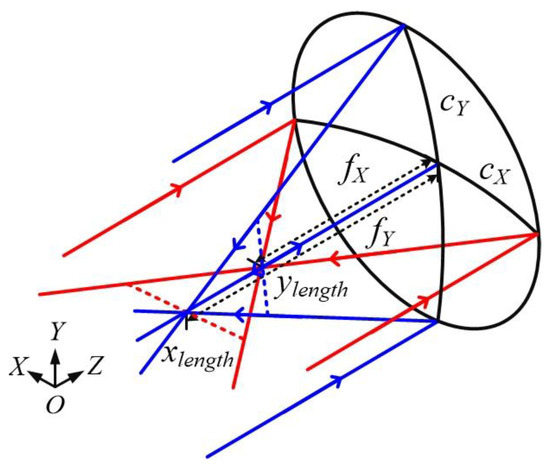
Figure 1.
Surface map of an anamorphic surface.
According to the two curvature characteristics, anamorphic surfaces are different from conventional symmetric surfaces. The parallel rays incident in an anamorphic surface no longer form a sharp point image but rather two strip images, namely, xlength and ylength, in the XOZ and YOZ planes, respectively. Moreover, in the paraxial region, if there is a ray incident in the XOZ or YOZ plane, the ray will only propagate in this plane. Based on these features, we calculate the initial structure of an anamorphic system.
In this study, the X and Y directions are defined as the directions for resolving spatial and spectral information, respectively. According to the anamorphic imaging relationship, the focal length FY in the Y direction is n times the focal length FX in the X direction, that is, FY = nFX.
A schematic diagram of the anamorphic system is shown in Figure 2; it is based on a Gregorian structure, and we analyze it in the XOZ and YOZ planes simultaneously. In the initial structural analysis, it is assumed that the rays from infinity and the marginal ray heights on the primary mirror (PM) are equal in the XOZ and YOZ planes (h1X = h1Y, and h1X and h1Y are the marginal ray heights on the PM in the X and Y directions, respectively). The stop is located on the front focal plane of the secondary mirror (SM) in the XOZ plane, and the system is telecentric in the XOZ plane. The PM assumes a large anamorphic effect, such that the marginal ray heights on the SM change significantly in two directions (h2X > h2Y, and h2X and h2Y are the marginal ray heights on the SM in the X and Y directions, respectively). The parallel rays are first imaged by the PM at different positions in the XOZ and YOZ planes between the PM and the SM; there is obvious astigmatism. Thus, SM provides aberration compensation for the system such that the two intermediate images at different positions are re-imaged at the same position.
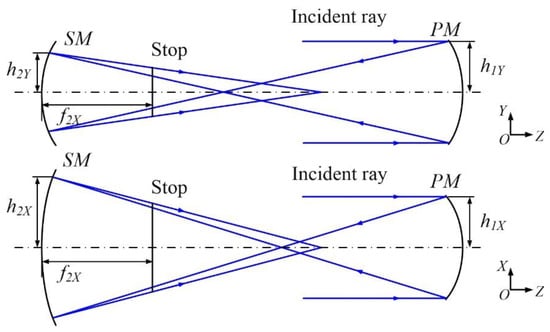
Figure 2.
Schematic diagram of the anamorphic system in the X and Y directions.
According to the Gaussian formula and primary aberration theory [26], the primary aberration formula for spherical, coma, astigmatism, field curvature, and distortion that satisfies the Gregorian anamorphic structure is as follows:
where αi is the system blocking ratio (αi = h2i/h1i), βi is the magnification of the SM; and −e1i2 and −e2i2 are the aspheric coefficients of the PM and SM, respectively (i = X, Y).
The structure parameters can be written as follows:
where Fi is the total focal length of the system; R1i and R2i are the radii of the curvatures of the PM and SM, respectively; di is the distance between the two mirrors; and li′ is the distance between the SM and the image plane.
First, we determined the initial structural parameters in the X direction. The system constraints include the diameter of the entrance pupil and the relative aperture of the PM in the X direction. When the specifications of the system are determined, according to Equations (1) and (2), the radii of the curvatures R1X and R2X of the PM and SM, the aspheric coefficients −e1X2 and −e2X2 of the PM and SM, the distance dX between the two mirrors, and the distance lX′ between the SM and the image plane in the X direction can be calculated.
Thereafter, we determined the initial structural parameters in the Y direction. The distance between the two mirrors and the image position were determined when solving the initial structure in the X direction; that is, dX = dY, lX′ = lY′, where dY is the distance between the two mirrors, and lY′ is the distance between the SM and the image plane in the Y direction. Thus, the other variables in the Y direction were the radii of the curvatures and aspheric coefficients.
Because FY = nFX, the relationship between the radii of the curvatures of the PM and SM in the X and Y directions can be obtained as follows:
where R1Y and R2Y are the radii of the curvatures of the PM and SM in the Y direction, respectively. According to Equation (3), provided the radii of the curvatures R1X and R2X are determined, the radii of the curvatures R1Y and R2Y can be obtained as follows:
where αX is the blocking ratio and βX is the magnification of the SM in the X direction. Therefore, the system blocking ratio αY and the magnification of the SM βY in the Y direction can be described as follows:
Thereafter, the aspheric coefficients −e1Y2 and −e2Y2 of the PM and SM in the Y direction can be extracted using Equations (1) and (5).
After obtaining the parameters of the anamorphic system, the initial structure with Biconic surfaces can be simulated. The Biconic expression is as follows:
Among them
where cX and cY are the curvatures of the mirror in the X and Y directions, respectively; RX and RY are the radii of curvatures of the mirror in the X and Y directions, respectively; kX and kY are the conic constants of the mirror in the X and Y directions, respectively; −eX2 and −eY2 are the aspheric coefficients of the mirror in the X and Y directions, respectively.
According to FY = nFX and Equations (3) and (7), the relationship between the curvatures of the PM and the SM in the X and Y directions can be obtained as follows:
where c1X, c2X, c1Y, and c2Y are the curvatures of the PM and SM in the X and Y directions. Furthermore, the relationship between the curvatures can also be expressed as follows:
2.2. Conversion Surface Type
The Biconic surface can be applied well to a coaxial system. For off-axis systems, the ability to correct aberrations is limited because it is symmetrical about the XOZ and YOZ planes. To improve the design freedom, we converted the Biconic surface into the XY polynomial surface. The XY polynomial freeform surface is formed based on adding polynomials to a quadratic surface, and it has the advantage of matching the description of numerical control optical manufacture [7]. Since the system we designed was symmetric about the YOZ plane, the coefficients of odd items of x in the XY polynomial were zero. The XY polynomial can be written as follows:
where c is the curvature, k is the conic constant of the freeform surface, and Aj (j = 1, 2, 3…) are the coefficients of the XY polynomial.
In the XY polynomial expression, the first term is a quadratic surface equation, and the radius of the curvature is expressed as follows:
The surface fitted by the first term of the XY polynomial is rotationally symmetrical, whereas the Biconic surface is non-rotationally symmetrical. Therefore, it is necessary to increase the freeform terms of the XY polynomial to compensate for the surface deviation caused by the surface conversion.
The A3x2 term is a parabolic surface equation, and a surface map of the A3x2 term is shown in Figure 3, where cX′ and cY′ are the curvature of the parabolic surface in the X and Y directions, respectively, and fX′ is the focal length of the parabolic surface in the X direction. The curvature of the surface in the YOZ plane is zero (cY′ = 0), and the radius of the curvature in the XOZ plane is expressed as follows:
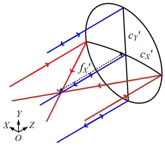
Figure 3.
Surface map of the A3x2 term.
In particular, the radius of the curvature of the XY polynomial surface is determined by the radius of the curvature of the quadratic term and the coefficients of the terms. Adding the A3x2 term can modify the curvature of the surface in the X direction, causing a change in the surface’s focal power in the X direction. Therefore, the focal power of the XY polynomial surface in the X direction can be approximately expressed as follows:
where φX is the focal power of the XY polynomial surface in the X direction, φ1 is the focal power of the quadratic term of the XY polynomial in the X direction, and φ2 is the focal power of the A3x2 term of the XY polynomial in the X direction (φ = 1/f, where φ is the focal power of the surface, and f is the focal length).
Then, according to Equations (8)–(11), the radius of the curvature RX and the coefficient A3 can be approximately written as follows:
Likewise, the relationship between the radius of the curvature RY and the coefficient A5 can be approximated as follows:
The relationship between the radii of the curvatures (RX and RY) of the Biconic surface and the terms of the XY polynomial was determined, and then we discussed the relationship between the conic coefficients (kX and kY) of the Biconic surface and the terms of the XY polynomial. We performed Taylor expansions for the expressions of the Biconic and XY polynomial surfaces. By specifying an expansion point (x = 0, y = 0), the four-order Taylor expansion of Equation (6) near the expansion point can be expressed as:
where O (x4, y4) is the remainder. Similarly, according to Equations (8), (12) and (13), the XY polynomial with quadratic, x2, y2, x4, and y4 terms can be expressed as follows:
where O′ (x4, y4) is the remainder. Then, according to Equations (14) and (15), the relationship between the conic constants kX and kY and the polynomial coefficients A10 and A14 can be approximated as follows:
2.3. Optimization Process
Based on the above analysis, an initial anamorphic structure with XY polynomials can be obtained. Moreover, system optimization is started after the above work.
The design of ultrawide FOV systems is made possible by the effective asymmetric aberration correction abilities of freeform surfaces. However, the optimization process is inefficient due to the large number of terms of the XY polynomial and the lack of a clear optimization theory as a guide. To solve this problem, we choose the Zernike polynomial as the optimization guide, which has a correspondence with the aberrations [27,28,29,30] and a conversion relationship with the XY polynomials, such as astigmatism (Z5, Z6) and coma (Z7, Z8), as follows:
In the optimization process, it is required to first identify which aberrations exist during the design process. Then, the corresponding XY polynomial terms are added to correct these aberrations. Freeform surfaces become progressively more complex, and the power of freeform terms increases from low to high. A flow chart of the design method of freeform anamorphic systems with an ultrawide FOV is shown in Figure 4.
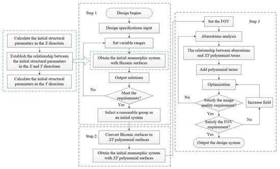
Figure 4.
Flow chart of design method of freeform anamorphic systems with ultrawide FOV.
3. Design Example
In this section, a UFOTAS with high performance is designed based on the method proposed in Section 2. The specifications are summarized in Table 1, and its spectral range is 270 mm–2400 mm, which includes UV, UVIS, NIR, and SWIR. The FOV is 110° in the X direction, where the range is from −55° to 55°; the FOV is 0.24° in the Y direction, where the range is from 0° to 0.24°; the F-numbers are 10 and 12 in the X and Y directions, respectively; and the entrance pupil is elliptical. The design can be used in a push-broom system, and when it orbits at an orbit height of circa 800 km, its image swath width can reach about 2700 km.

Table 1.
Specifications of the UFOTAS.
First, we determined the range of the system length and image plane; the total length of the system is required to be less than 300 mm. Then, according to the specifications (the F-number, focal length, and anamorphic ratio), a series of initial freeform anamorphic structure parameters were solved using a computer, and a reasonable group was selected from them for further optimization. Next, the PM was set to 6 mm Y-decenter and the SM was set to −3 mm Y-decenter to make the system unobstructed. The layout of the initial structure is shown in Figure 5.
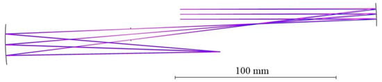
Figure 5.
The layout of the initial freeform anamorphic system.
Further optimization was performed on the constructed anamorphic system using the optical design software. The FOV in the system was set, and the aberrations were analyzed. The variations in coma and astigmatism with the FOV are shown in Figure 6. When the FOV was wider than 15°, the astigmatism of the system was more serious than the coma. Therefore, astigmatism was the most significant aberration to correct. Through analyses, we set the astigmatism contribution terms of the XY polynomial as variables to eliminate this aberration until the requirement was reached. The analysis and optimization methods used for astigmatism are also applicable to other aberrations, so the correction of other aberrations was not performed here.
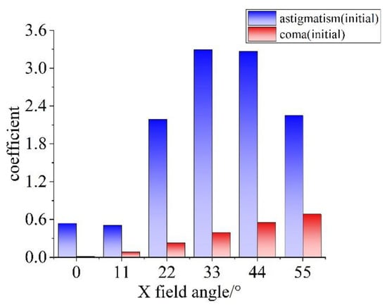
Figure 6.
Aberrations of the initial structure.
The system is symmetric about the YOZ plane; therefore, the x2myn term of the XY polynomial was selected for optimization. To reduce the complexity of the surface shape and to avoid manufacturing difficulties, low-order polynomial terms were selected (2m + n ≤ 6). Considering that the x2, x4, and x4y2 terms are related to astigmatism, the x2y term can correct coma, and the x2y2 term contributes to spherical and defocus. Therefore, in addition to the x2 and x4 terms, the x2y, x2y2, and x4y2 terms were added to the optimization in order to help refine the system. It should be emphasized that although the freeform surface provides more ability to correct aberrations, it is not infinite, so the specifications of the anamorphic system need to be reasonable.
In the optimization process, in addition to setting the structure parameters and the XY polynomial terms as variables, some constraints must also be added. Since the system is required to be telecentric in the XOZ plane, this was achieved by controlling the angle between the main ray of the emergent rays and the image plane close to zero. Moreover, the X-tilt and Y-decenter of each mirror and image plane were also set as variables, adding more design freedom to the system and ensuring that the system is unobstructed.
With the optimization completed, a schematic diagram of the UFOTAS is shown in Figure 7. The direction of the ultrawide FOV is the spatial dimension of the system, and the direction perpendicular to it is the spectral dimension. Figure 8a shows the RMS and 100% spot radius for all FOVs. Figure 8b shows the modulation transfer function (MTF) in the X direction, and Figure 8c shows the MTF in the Y direction. Figure 9 shows the coma and astigmatism of the UFOTAS. After optimization, the aberration coefficient of the astigmatism of each FOV was less than 0.26, and the aberration coefficient of the coma for each FOV was less than 0.18. Compared with the aberration coefficients of the initial structure, the aberrations of the edge FOV were significantly corrected.
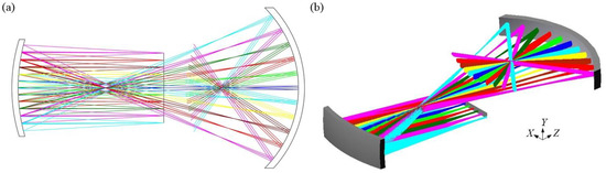
Figure 7.
Final designed layout of the compact UFOTAS: (a) layout in XOZ plane, (b) 3D layout.
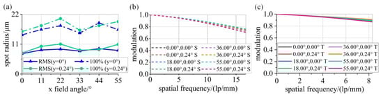
Figure 8.
Performance analysis results of the UFOTAS: (a) spot diagram, (b) MTF in the X direction, (c) MTF in the Y direction.
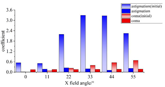
Figure 9.
Aberrations of the system after optimization.
The telescope has a magnification of 0.6 mm/° in the X direction and 1.2 mm/° in the Y direction, which fulfills our requirement for the anamorphic system. The system is an almost f-θ system: the field angle has a linear relationship with the position of the imaging point (h = f·θ, where h is the transverse distance between the imaging point and the optic axis, and θ is the field angle). Thus, the edge FOV along the long-slit direction also has a magnification of 0.6 mm/°.
The freeform surface coefficients of the PM and SM are shown in Table 2. The overall volume of the UFOTAS was approximately 140 mm (X) × 35 mm (Y) × 270 mm (Z); the size of the PM was approximately 140 mm × 10 mm; and the size of the SM was approximately 80 mm × 15 mm. To evaluate the freeform surfaces, we plotted the surface maps of the PM and SM as shown in Figure 10, and we calculated the sag deviation of each surface from its best-fit sphere, as shown in Figure 11.
Table 2.
Freeform surface coefficients.
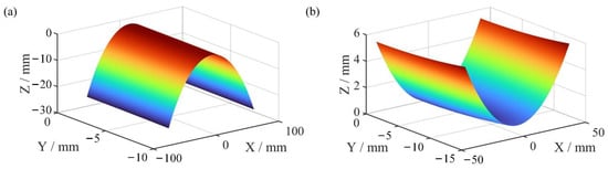
Figure 10.
Surface maps: (a) PM, (b) SM.
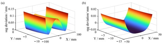
Figure 11.
Sag deviation from the best-fit sphere: (a) PM, (b) SM.
4. Discussion
In this paper, a method for solving the initial structure of a freeform anamorphic system was proposed. According to the method in Section 2.1 and Section 2.2, a program can be written. Then, after entering the specifications of the anamorphic system, a series of solutions will be automatically calculated. Moreover, an appropriate solution can be selected for further optimization. Compared with the traditional method that relies on optical design software to gradually optimize the focal length, design efficiency is improved and the designer experience for anamorphic systems is reduced. Furthermore, the initial structure with XY polynomials provides a good starting point for an ultrawide FOV design. Designing an ultrawide FOV system is a challenge, and we used Zernike polynomials to guide optimization, which helped us to correct the FOV-related aberrations and improve optimization efficiency.
TROPOMI, as an ultrawide FOV anamorphic telescope successfully applied to atmospheric remote sensing, has a very important learning value and reference significance. Therefore, we referred to TROPOMI’s specifications and simulated the UFOTAS as an example. As shown in Table 3, our design achieved an ultrawide FOV anamorphic telescope with a lower-order XY polynomial. To obtain a small image spot size, we increased the F-number. The resolutions of the UFOTAS and TROPOMI are shown in Figure 12. It can be seen that the UFOTAS has a higher resolution and remains much more constant over the field. The maximum sag deviation between TROPOMI’s mirror and its best-fit spherical surface is approximately 0.3 mm, while the maximum sag deviation of the UFOTAS is approximately 0.15 mm. The surfaces in the UFOTAS have gentle shapes, which can greatly reduce the manufacturing difficulty and cost. As for the design results shown in Section 3, the simulated UFOTAS using the method mentioned in this study has good image quality and meets the requirements of an ultrawide FOV, with an anamorphic and compact structure. This demonstrates that the design method described in this study is feasible.
Table 3.
Design comparison of UFOTAS and TROPOMI.
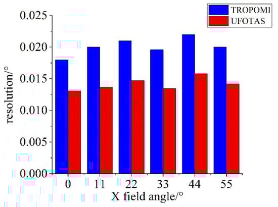
Figure 12.
Resolution comparison between UFOTAS and TROPOMI.
5. Conclusions
This study presented a design method for freeform anamorphic telescopes with an ultrawide FOV. This method can effectively obtain an anamorphic telescope with XY polynomial surfaces as a good starting point for an ultrawide FOV design. Referring to TROPOMI’s specifications and using the Zernike polynomial to guide optimization, the UFOTAS with a focal length of 34 mm × 68 mm and an FOV of 110° × 0.24° was designed. The simulation shows that the UFOTAS uses a sixth-order XY polynomial to obtain a low sag deviation of the mirror from its best-fit sphere and a good imaging performance. In conclusion, atmospheric remote sensing is a vital development. To obtain more adequate observation data from satellites, we should enhance the spectral sampling rate of the system; an anamorphic telescope provides an effective method. The design method in this study of an ultrawide FOV off-axis anamorphic telescope and its simulation can be used as a reference in this field.
6. Patents
Shi, Y.; Zheng, Y.; Lin, C.; Ji, Z.; Zhang, J.; Han, Y. A method for solving the initial structure of an anamorphic system and converting between freeform surface types. CN202111014855.6.
Author Contributions
Conceptualization, Y.S. and Y.Z.; methodology, Y.S.; software, Y.S.; validation, Y.S., J.Z., C.L. and Z.J.; formal analysis, Y.S. and Y.H.; investigation, Y.S.; resources, Y.Z.; data curation, Y.S.; writing—original draft, Y.S.; writing—review and editing, J.Z.; visualization, L.T., and D.H.; supervision, Y.Z.; project administration, Y.Z.; funding acquisition, Y.Z. All authors have read and agreed to the published version of the manuscript.
Funding
This research was funded by the National Key Research and Development Program of China (No. 2021YFB3901000, 2021YFB3901004).
Institutional Review Board Statement
Not applicable.
Informed Consent Statement
Not applicable.
Data Availability Statement
Not applicable.
Conflicts of Interest
The authors declare no conflict of interest.
References
- Roscoe, H.K.; Fish, D.J.; Jones, R.L. Interpolation errors in UV–visible spectroscopy for stratospheric sensing: Implications for sensitivity, spectral resolution, and spectral range. Appl. Opt. 1996, 35, 427–434. [Google Scholar] [CrossRef] [PubMed]
- Chance, K. Analysis of BrO measurements from the Global Ozone Monitoring Experiment. Geophys. Res. Lett. 1998, 25, 3335–3338. [Google Scholar] [CrossRef]
- Chance, K.; Kurosu, T.P.; Sioris, C.E. Undersampling correction for array detector-based satellite spectrometers. Appl. Opt. 2005, 44, 1296–1304. [Google Scholar] [CrossRef] [PubMed]
- Gong, T.; Jin, G.; Zhu, J. Point-by-point design method for mixed-surface-type off-axis reflective imaging systems with spherical, aspheric, and freeform surfaces. Opt. Express 2017, 25, 10663–10676. [Google Scholar] [CrossRef] [PubMed]
- Haring, R.E.; Pollock, R.; Cross, R.M. Wide-Field-of-View Imaging Spectrometer (WFIS) engineering model laboratory tests and field demonstration. Proc. SPIE 2003, 5152, 51–60. [Google Scholar]
- Levelt, P.F.; Oord, G.; Dobber, M.R.; Malkki, A.; Visser, H.; Vries, J.; Stammes, P.; Saari, H. The ozone monitoring instrument. IEEE Trans. Geosci. Remote Sens. 2006, 44, 1093–1101. [Google Scholar] [CrossRef]
- Zhang, X.; Zheng, L.; He, X.; Wang, L.; Zhang, F.; Yu, S.; Shi, G.; Zhang, B.; Liu, Q.; Wang, T. Design and fabrication of imaging optical systems with freeform surfaces. Proc. SPIE 2012, 8486, 848607. [Google Scholar]
- Meng, Q.; Wang, H.; Liang, W.; Yan, Z.; Wang, B. Design of off-axis three-mirror systems with ultrawide field of view based on an expansion process of surface freeform and field of view. Appl. Opt. 2019, 58, 609–615. [Google Scholar] [CrossRef]
- Thompson, P.K.; Rolland, J.P. Freeform Optical Surfaces: A Revolution in Imaging Optical Design. Opt. Photonics News 2012, 23, 30–35. [Google Scholar] [CrossRef]
- Fuerschbach, K.; Rolland, J.P.; Thompson, K.P. A new family of optical systems employing φ-polynomial surfaces. Opt. Express 2011, 19, 21919–21928. [Google Scholar] [CrossRef]
- Bauer, A.; Rolland, J.P. Visual space assessment of two all-reflective, freeform, optical see-through head-worn displays. Opt. Express 2014, 22, 13155–13163. [Google Scholar] [CrossRef] [PubMed]
- Chen, L.; Gao, Z.; Ye, J.; Cao, X.; Xu, N.; Yuan, Q. Construction method through multiple off-axis parabolic surfaces expansion and mixing to design an easy-aligned freeform spectrometer. Opt. Express 2019, 27, 25994–26013. [Google Scholar] [CrossRef] [PubMed]
- Shen, Z.; Yu, J.; Song, Z.; Chen, L.; Yuan, Q.; Gao, Z.; Pei, S.; Liu, B.; Ye, J. Customized design and efficient fabrication of two freeform aluminum mirrors by single point diamond turning technique. Appl. Opt. 2019, 58, 2269–2276. [Google Scholar] [CrossRef]
- Zhang, J.; Lin, C.; Ji, Z.; Wu, H.; Li, C.; Du, B.; Zheng, Y. Design of a compact hyperspectral imaging spectrometer with freeform surface based on astigmatism. Appl. Opt. 2020, 59, 1715–1725. [Google Scholar] [CrossRef] [PubMed]
- Xie, Y.; Mao, X.; Li, J.; Wang, F.; Wang, P.; Gao, R.; Li, X.; Ren, S.; Xu, Z.; Dong, R. Optical design and fabrication of an all-aluminum unobscured two-mirror freeform imaging telescope. Appl. Opt. 2020, 59, 833–840. [Google Scholar] [CrossRef]
- Qin, Z.; Qi, Y.; Ren, C.; Wang, X.; Meng, Q. Desensitization Design Method for Freeform TMA Optical Systems Based on Initial Structure Screening. Photonics 2022, 9, 544. [Google Scholar] [CrossRef]
- Zhang, J.; Zheng, Y.; Lin, C.; Ji, Z.; Wu, H. Analysis method of the Offner hyperspectral imaging spectrometer based on vector aberration theory. Appl. Opt. 2021, 60, 264–275. [Google Scholar] [CrossRef]
- Zhang, B.; Jin, G.; Zhu, J. Towards automatic freeform optics design: Coarse and fine search of the three-mirror solution space. Light Sci. Appl. 2021, 10, 11. [Google Scholar] [CrossRef]
- Yang, T.; Jin, G.; Zhu, J. Automated design of freeform imaging systems. Light Sci. Appl. 2017, 6, e1708. [Google Scholar] [CrossRef]
- Jannick, P.R.; Matthew, A.D.; Thomas, J.S.; Chris, E.; Aaron, B.; John, C.L.; Konstantinos, F. Freeform optics for imaging. Optica 2021, 8, 161–176. [Google Scholar]
- Dmitry, R.; Jose, S. A method for the design of unsymmetrical optical systems using freeform surfaces. Proc. SPIE 2017, 10590, 105900V. [Google Scholar]
- José, S. Method of confocal mirror design. Opt. Eng. 2019, 58, 015101. [Google Scholar]
- Matthias, B.; Johannes, H.; Thomas, P.; Christoph, D.; Andreas, G.; Sebastian, S.; Daniela, S.; Uwe, D.; Stefan, R.; Ramona, E.; et al. Development, fabrication, and testing of an anamorphic imaging snap-together freeform telescope. Appl. Opt. 2015, 54, 3530–3542. [Google Scholar]
- Nijkerk, D.; Venrooy, B.; Doorn, P.; Henselmans, R.; Draaisma, F.; Hoogstrate, A. The TROPOMI Telescope. Proc. SPIE 2017, 10564, 105640Z. [Google Scholar]
- Veefkind, J.P.; Aben, I.; Mcmullan, K.; Förster, H.; Vries, J.; Otter, G.; Claas, J.; Eskes, H.J.; Haan, J.F.; Kleipool, Q.; et al. TROPOMI on the ESA Sentinel-5 Precursor: A GMES mission for global observations of the atmospheric composition for climate, air quality and ozone layer application. Remote Sens. Environ. 2012, 120, 70–83. [Google Scholar] [CrossRef]
- Pan, J. The Design, Manufacture and Test of the Aspherical Optical Surfaces; Soochow University Press: Suzhou, China, 2001; pp. 11–14. [Google Scholar]
- Fuerschbach, K.; Rolland, P.J.; Thompson, P.K. Theory of aberration fields for general optical systems with freeform surfaces. Opt. Express 2014, 22, 26585–26606. [Google Scholar] [CrossRef]
- Yang, T.; Cheng, D.; Wang, Y. Aberration analysis for freeform surface terms overlay on general decentered and tilted optical surfaces. Opt. Express 2018, 26, 7751–7770. [Google Scholar] [CrossRef]
- Karcı, Ö.; Yeşiltepe, M.; Arpa, E.; Wu, Y.; Ekinci, M.; Rolland, P.J. Experimental investigation in nodal aberration theory (NAT): Separation of astigmatic figure error from misalignments in a Cassegrain telescope. Opt. Express 2021, 29, 19427–19440. [Google Scholar] [CrossRef]
- Reimers, J.; Bauer, A.; Thompson, K.P.; Rolland, J.P. Freeform spectrometer enabling increased compactness. Light Sci. Appl. 2017, 6, e17026. [Google Scholar] [CrossRef]
Publisher’s Note: MDPI stays neutral with regard to jurisdictional claims in published maps and institutional affiliations. |
© 2022 by the authors. Licensee MDPI, Basel, Switzerland. This article is an open access article distributed under the terms and conditions of the Creative Commons Attribution (CC BY) license (https://creativecommons.org/licenses/by/4.0/).