Tailoring the Axial Intensity of Bessel Beams for Ionizing Radiation and TGV Applications Using Different Optimized Nonlinear Phases

Abstract

This work presents a refined theoretical and numerical framework for shaping the axial intensity of finite-energy Bessel–Gaussian beams through programmable nonlinear phase modulation. Starting from the scalar Fresnel diffraction integral, we reformulate the propagation of a Gaussian-apodized axicon beam using a dimensionally consistent stationary-phase method. This analysis directly relates the radial phase gradient to the saddle-point trajectory, phase curvature, and on-axis intensity distribution. A Gaussian phase modulation (GPM) serves as a reference design to achieve a flattop axial profile while preserving the characteristic transverse Bessel ring structure. This work is validated against beam propagation simulations and previously reported spatial light modulator (SLM) experiments, confirming its accuracy within the paraxial regime. A parametric study then clarifies the scaling of wavelength, beam waist, axicon angle, and refractive index for extended focusing. Beyond standard GPM, several alternative nonlinear phase functions are systematically compared. High-performing profiles must replicate not only the amplitude scale but, more importantly, the radial phase-gradient structure of the Gaussian reference, which governs energy redistribution from annular regions to the axis. The results identify smooth, localized nonlinear functions as promising candidates for stable flattop Bessel beam generation. The proposed framework offers a flexible optical design for applications such as through-glass via (TGV) micromachining and light-sheet illumination, while prospective high-intensity laser plasma uses remain beyond the present linear model.

1. Introduction

Extended axial focusing is a central requirement in modern structured-light applications because it allows optical energy to be delivered over distances that are much longer than the Rayleigh range of an ordinary Gaussian focus. In femtosecond laser micromachining, this capability is particularly important for through-glass vias (TGVs) and through-ceramic vias (TCVs), where nonuniform energy deposition can produce tapered sidewalls, irregular modification tracks, and reduced processing repeatability [1,2]. Beyond microfabrication, controlled axial intensity profiles are also relevant to light-sheet microscopy, optical trapping, waveguide writing, and laser-assisted generation of plasma or radiation sources, provided that the optical model is coupled to the appropriate material or plasma-response physics.

Bessel beams provide one of the most useful routes toward extended focusing. They were introduced as nondiffracting solutions of the scalar Helmholtz equation and can maintain an approximately invariant transverse profile over a finite propagation distance when physically realized as aperture-limited quasi-Bessel beams [3,4,5]. A zero-order Bessel beam consists of a bright central lobe surrounded by concentric rings, while higher-order Bessel beams contain an annular intensity distribution associated with orbital angular momentum. Although an ideal Bessel beam would require infinite transverse energy, experimentally realizable Bessel–Gaussian beams retain the key advantages of a long depth of focus, resistance to diffraction, and self-healing after partial obstruction [5,6,7]. These properties make them attractive for laser ablation and selective laser etching, in which long and stable modification holes can improve axial uniformity compared with a tightly focused Gaussian beam [2,8].

Two different axial-control regimes are relevant to the present work. The first is flat-top or uniform axial focusing, in which the goal is to maintain nearly constant on-axis intensity over a prescribed distance. This regime is directly useful for TGV/TCV drilling and light-sheet illumination because it reduces the variation in deposited energy along the processing or imaging depth. The second is abrupt axial focusing, in which the beam remains relatively weak over most of its trajectory and then concentrates sharply near a designed position. Such abruptly focused beams are not equivalent to flat-top Bessel beams, but they are part of the broader concept of axial intensity engineering and can be useful when localized energy deposition is desired [9,10]. In this research, the flat-top Bessel-beam design is treated as the primary objective, whereas abrupt focusing is discussed separately as a distinct nonlinear-phase design target.

The relevance of extended and shaped focusing also extends to high-field and nuclear-related radiation applications. For example, at 1030 nm [11], the photon energy is only approximately 1.20 eV, which is far below typical atomic ionization potentials; therefore, near-infrared femtosecond pulses do not ionize through single-photon absorption [12]. However, when tightly or axially concentrated to intensities on the order of ${10}^{14} \mathrm{W}\hspace{0.17em}\mathrm{c}{\mathrm{m}}^{-2}$ or higher, the optical electric field can drive multiphoton, tunneling, and over-the-barrier ionization processes [13]. Long-depth Bessel or Bessel-like beams have therefore been investigated as drivers for optical-field-ionized plasma channels and hydrodynamic plasma waveguides, which are important for guiding high-intensity laser pulses over many Rayleigh lengths in multi-GeV laser wakefield acceleration (LWFA) [14,15,16,17]. In this research, a flatter axial intensity profile may help produce a more uniform plasma distance, although full validation requires plasma-dynamics simulations beyond the scalar propagation model used here.

Structured beams are also relevant to gamma-ray and compact X-ray generation. In laser-plasma and inverse-Compton interaction schemes, the spatial structure, polarization, and orbital angular momentum of the optical driver can influence the angular momentum and brightness of the emitted high-energy radiation [18]. In addition, Bessel light beams have been proposed as optical undulators for free-electron-laser concepts, where a co-propagating structured laser field can impose an oscillatory transverse force on an electron beam and potentially reduce the effective undulator period [19]. These high-energy examples motivate the development of robust beam-shaping methods, but they should be interpreted as prospective applications of the optical fields rather than direct outcomes of the present linear scalar model.

Bessel–Gaussian beams are commonly generated by imposing a conical wavefront on a Gaussian input. This can be achieved with refractive or reflective axicons, annular apertures, or computer-generated holograms displayed on a spatial light modulator (SLM) [11,20,21,22,23,24]. Conventional axicons are robust and simple, but their fixed geometry limits dynamic control over the axial intensity. Moreover, axial oscillations can arise from finite-aperture effects, axicon-tip imperfections, and diffraction from the input beam envelope. Alternative approaches, such as illuminating an axicon with hollow Gaussian beams, have also demonstrated segmented zero-order Bessel beams with tunable ranges and reduced on-axis modulation [2]. The SLM-based strategy adopted here is complementary because it enables reconfigurable, phase-only control without replacing physical optics.

Previous studies have shown that the axial distribution of a Bessel-like beam can be engineered by tailoring the radial phase or spatial spectrum. Examples include apodized axicons, logarithmic or generalized axicon profiles, phase-only holograms, and iterative or direct holographic methods for shaping the on-axis amplitude [25,26,27]. More recently, programmable structured-light generation has also benefited from machine-learning-assisted diffractive design and advanced coherent detection of vectorial structured light [28,29]. These developments highlight the broader trend toward programmable, high-fidelity control of optical fields in both amplitude and phase.

Recently, Elsharkawi and Lo proposed a Gaussian phase modulation (GPM) added to the axicon phase to generate a Bessel beam with a flat-top axial intensity profile, and validated the method using beam-propagation simulations [11,24,30,31] and experiments [31]. The novelty of this work is not simply the application of GPM, but rather the systematic extension of the framework to alternative nonlinear radial phase profiles—unlike previous studies [11]—and a comparative assessment of their capacity to reproduce or enhance the flat-top reference response, making the approach well-suited for free-electron laser and laser wakefield acceleration applications. Specifically, this work examines how the radial phase-gradient structure controls the saddle-point trajectory and therefore the redistribution of optical power along the propagation axis. By clarifying this transport mechanism, the study provides a design pathway for selecting nonlinear phase functions that preserve the Bessel-like transverse structure while improving axial uniformity for micromachining, imaging, and high-field beam-delivery applications.

2. GPM for Different Input Beams

2.1. Gaussian Beam Formulation Multiplied by a Gaussian Phase Function

The electric field of a fundamental Gaussian beam at the waist plane $z=0$ is written as [32]:

$$E\left(r,0\right)=\mathrm{e}\mathrm{x}\mathrm{p}\left[-{\left({\displaystyle \frac{r}{w_0}}\right)}^2\right], r=\sqrt{x^2+y^2}$$

(1)

Here, $r$ is the radial coordinate at the input plane and $w_0$ is the beam-waist radius. To avoid ambiguity between the input radius and the observation radius, the transverse coordinate at a propagation distance $z$ is denoted by $\rho$. For a radially symmetric field, the full scalar Fresnel integral reduces to the cylindrical Fresnel–Hankel form

$$E\left(\rho ,z\right)={\displaystyle \frac{2\pi e^{jkz}}{j\lambda z}}\mathrm{e}\mathrm{x}\mathrm{p}\left({\displaystyle \frac{jk{\rho }^2}{2z}}\right){\int }_0^{\mathrm{\infty }}E\left(r,0\right)\mathrm{e}\mathrm{x}\mathrm{p}\left({\displaystyle \frac{jk{r}^2}{2z}}\right)J_0\left({\displaystyle \frac{k\rho r}{z}}\right)r\hspace{0.17em}dr$$

(2)

Equation (2) contains the angular integration term $J_0\left(k\rho r/z\right)$ and is therefore valid for the transverse field, not only for the on-axis field. The on-axis expression follows only after setting $\rho =0$, where $J_0\left(0\right)=1$. Substitution of Equation (1) into Equation (2) yields the standard Gaussian-beam solution:

$$E_G\left(\rho ,z\right)=e^{jkz}{\displaystyle \frac{w_0}{w\left(z\right)}}\mathrm{e}\mathrm{x}\mathrm{p}\left[-{\displaystyle \frac{{\rho }^2}{w^2\left(z\right)}}\right]\mathrm{e}\mathrm{x}\mathrm{p}\left[-j{\displaystyle \frac{k{\rho }^2}{2R\left(z\right)}}+j\zeta \left(z\right)\right]$$

(3)

The beam parameters are

$$w\left(z\right)=w_0\sqrt{1+{\left({\displaystyle \frac{z}{z_R}}\right)}^2}, R\left(z\right)=z\left[1+{\left({\displaystyle \frac{z_R}{z}}\right)}^2\right], \zeta \left(z\right)={\mathrm{t}\mathrm{a}\mathrm{n}}^{-1}\left({\displaystyle \frac{z}{z_R}}\right), z_R={\displaystyle \frac{\pi w_0^2}{\lambda }}$$

(4)

A phase-only SLM can modify the wavefront without directly changing the incident amplitude. In this preliminary case, the nonlinear phase is taken as a centered Gaussian phase modulation ${\psi }_G\left(r\right)=C\mathrm{e}\mathrm{x}\mathrm{p}\left[-{\left({\displaystyle \frac{r}{w_0}}\right)}^2\right]$, where $C$ is a dimensionless phase amplitude in radians. The modulated input field is

$$E\left(r,0;C\right)=\mathrm{e}\mathrm{x}\mathrm{p}\left[-{\left({\displaystyle \frac{r}{w_0}}\right)}^2\right]\mathrm{e}\mathrm{x}\mathrm{p}\left[-j{\psi }_G\left(r\right)\right]$$

(5)

Because the phase factor in Equation (5) is the exponential of a Gaussian function, it can be expanded exactly as

$$E\left(r,0;C\right)={\displaystyle {\sum }_{n=0}^{\mathrm{\infty }}}{\displaystyle \frac{{\left(-jC\right)}^n}{n!}}\mathrm{e}\mathrm{x}\mathrm{p}\left[-\left(n+1\right){\left({\displaystyle \frac{r}{w_0}}\right)}^2\right]$$

(6)

The linearity of Fresnel propagation allows each Gaussian term in Equation (6) to propagate independently. The $n$-th component has an effective waist $w_{n,0}=w_0/\sqrt{n+1}$ and the Rayleigh range $z_{R,n}=\pi w_{n,0}^2/\lambda$. Thus,

$$E\left(\rho ,z;C\right)=e^{jkz}{\displaystyle {\sum }_{n=0}^{\mathrm{\infty }}}{\displaystyle \frac{{\left(-jC\right)}^n}{n!}}{\displaystyle \frac{w_{n,0}}{w_n\left(z\right)}}\mathrm{e}\mathrm{x}\mathrm{p}\left[-{\displaystyle \frac{{\rho }^2}{w_n^2\left(z\right)}}\right]\mathrm{e}\mathrm{x}\mathrm{p}\left[-j{\displaystyle \frac{k{\rho }^2}{2R_n\left(z\right)}}+j{\zeta }_n\left(z\right)\right]$$

(7)

The quantities $w_n\left(z\right)$, $R_n\left(z\right)$, and ${\zeta }_n\left(z\right)$ are obtained from Equation (4) by replacing $w_0$ and $z_R$ with $w_{n,0}$ and $z_{R,n}$. The series is absolutely convergent for finite $C$ and can be truncated once the terms ${\left|C\right|}^n/n!$ become negligible. A normalized on-axis intensity may also be written in terms of Kummer’s confluent hypergeometric function as

$$I_N\left(0,z;C\right)={\displaystyle \frac{{\xi }^2}{1+{\xi }^2}}{{|}_1{F}_1\left(1-j\xi ;2-j\xi ;-jC\right)|}^2, \xi ={\displaystyle \frac{z_R}{z}}$$

(8)

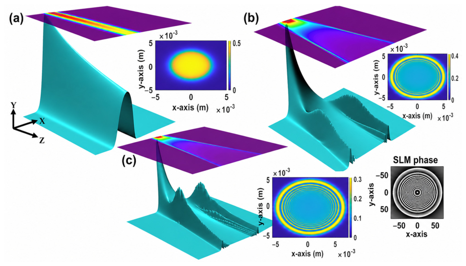
Figure 1 illustrates the propagation behavior of a Gaussian beam modified only by the GPM term for representative values of $C$. This preliminary case is useful for understanding how a nonlinear phase redistributes energy, but it should not be confused with the axicon-generated flat-top Bessel beam, which will be discussed in the next section. At small modulation, the beam remains close to a Gaussian focus. At larger modulation, radial phase gradients generate annular features and axial oscillations; however, a conical axicon term is still required to form a controlled Bessel–Gaussian beam with a designed extended axial response.

2.2. Zero-Order Bessel–Gaussian Beam Formulation with GPM Function

Finite-energy Bessel–Gaussian beams can be produced by imposing a conical phase on a Gaussian input beam. In practice, this conical phase may be introduced by a refractive axicon or, equivalently, by a computer-generated hologram displayed on a phase-only SLM. The phase-modulated Gaussian input is written as [30]

$$E\left(r,0\right)=A_0\mathrm{e}\mathrm{x}\mathrm{p}\left[-{\left({\displaystyle \frac{r}{w_0}}\right)}^2\right]\mathrm{e}\mathrm{x}\mathrm{p}\left[-j\psi \left(r\right)\right]$$

(9)

For a conventional axicon, or for an SLM programmed to emulate an axicon, the radial phase is linear in $r$:

$${\psi }_{\mathrm{a}\mathrm{x}}\left(r\right)=k_{t}r=k_0\left(n-1\right)\mathrm{t}\mathrm{a}\mathrm{n}\theta \hspace{0.17em}r, k_t=k_0\alpha , \alpha =\left(n-1\right)\mathrm{t}\mathrm{a}\mathrm{n}\theta$$

(10)

Here, $k_0=2\pi /\lambda$, $n$ is the refractive index of the axicon material, $\theta$ is the cone angle, and $\alpha$ is the axial slope. With total input power $P_0$, stationary-phase evaluation gives the standard Bessel–Gaussian intensity [30]:

$$I\left(\rho ,z\right)=I\left(0,z\right)J_0^2\left(k_t\rho \right), I\left(0,z\right)={\displaystyle \frac{8\pi P_{0}z{\alpha }^2}{\lambda w_0^2}}\mathrm{e}\mathrm{x}\mathrm{p}\left[-2{\left({\displaystyle \frac{\alpha z}{w_0}}\right)}^2\right]$$

(11)

Equation (11) shows that the transverse profile is Bessel-like, whereas the axial envelope is not uniform: the factor $z$ initially increases the intensity, while the finite Gaussian aperture later suppresses it. To redistribute optical energy along the propagation axis, a Gaussian phase modulation is added to the axicon phase,

$$\psi \left(r\right)=k_{t}r+C\mathrm{e}\mathrm{x}\mathrm{p}\left[-{\left({\displaystyle \frac{r}{w_0}}\right)}^2\right]$$

(12)

Using the sign convention in Equation (9), the dimensionally consistent reduced phase entering the stationary-phase analysis is

$$S\left(r;z\right)={\displaystyle \frac{r^2}{2z}}-\alpha r-{\displaystyle \frac{C}{k_0}}\mathrm{e}\mathrm{x}\mathrm{p}\left[-{\left({\displaystyle \frac{r}{w_0}}\right)}^2\right]$$

(13)

The stationary radius $r_s$ is determined by

$$S^{\mathrm{\prime }}\left(r_s;z\right)={\displaystyle \frac{r_s}{z}}-\alpha +{\displaystyle \frac{2C{r}_s}{k_0{w}_0^2}}\mathrm{e}\mathrm{x}\mathrm{p}\left[-{\left({\displaystyle \frac{r_s}{w_0}}\right)}^2\right]=0$$

(14)

and the corresponding curvature is

$$S″\left(r_s;z\right)={\displaystyle \frac{1}{z}}+{\displaystyle \frac{2C}{k_0{w}_0^2}}\mathrm{e}\mathrm{x}\mathrm{p}\left[-{\left({\displaystyle \frac{r_s}{w_0}}\right)}^2\right]\left[1-2{\left({\displaystyle \frac{r_s}{w_0}}\right)}^2\right]$$

(15)

For an isolated non-degenerate saddle point, the resulting intensity is

$$I\left(\rho ,z\right)\approx {\displaystyle \frac{8{\pi }^3{\left|A_0\right|}^2}{{\lambda }^2{z}^2}}{\displaystyle \frac{r_s^2\mathrm{e}\mathrm{x}\mathrm{p}\left[-2{\left(r_s/w_0\right)}^2\right]}{k_0\left|S″\left(r_s;z\right)\right|}}{J}_0^2\left({\displaystyle \frac{k_0{r}_s\rho }{z}}\right)$$

(16)

When $C=0$, Equation (14) gives $r_s=\alpha z$ and Equation (15) gives $S″=1/z$. With the Gaussian-power normalization ${\left|A_0\right|}^2=2P_0/\left(\pi w_0^2\right)$, Equation (16) reduces exactly to Equation (11). This confirms the consistency of the stationary-phase formulation. The GPM coefficient required to obtain an approximately uniform axial response can be estimated as

$$C_{\mathrm{o}\mathrm{p}\mathrm{t}}\approx 2.44{\displaystyle \frac{\left(n-1\right)w_0\mathrm{t}\mathrm{a}\mathrm{n}\theta }{\lambda }}$$

(17)

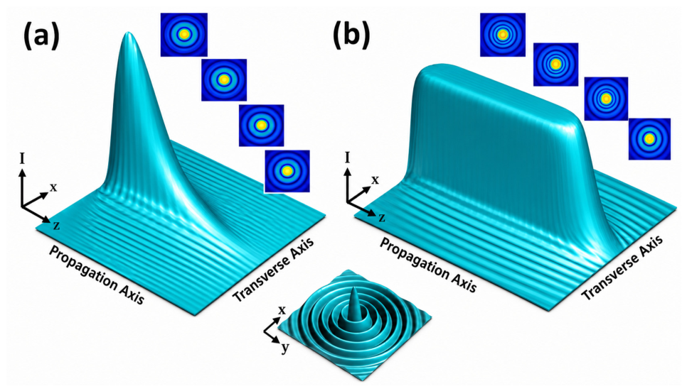
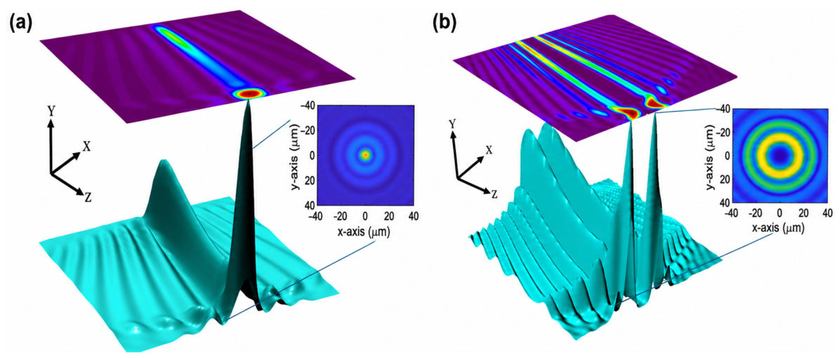
A three-dimensional schematic in Figure 2 compares the propagation of a standard Bessel–Gaussian beam with that of a GPM-modified beam using beam propagation method simulations [30,33,34]. The GPM case exhibits a substantially flatter axial region while retaining the characteristic transverse Bessel-like ring pattern.

3. Validation of the GPM-Modified Bessel Beam

3.1. Validation Against Analytical, BPM, and Experimental Results

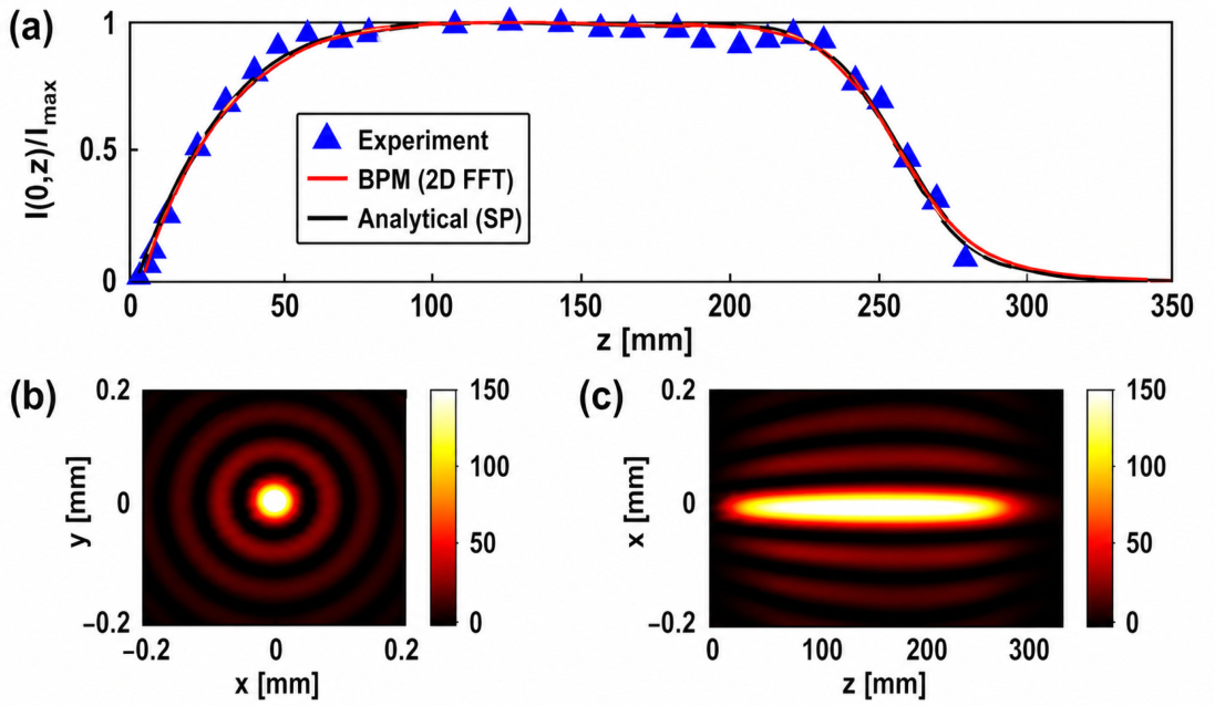
Figure 3 compares the normalized axial-intensity response of a zero-order Bessel–Gaussian beam generated with the combined axicon and GPM phase. Three datasets are shown: the analytical stationary-phase prediction from Equation (15), a beam-propagation simulation, and experimental data adapted from the SLM-based measurements reported in Ref. [35]. The experimental curve is therefore used here as a benchmark for validation and comparison rather than as a newly acquired measurement in this work. This clarification addresses the distinction between original calculations in this work and data reproduced or adapted from earlier studies [31,35].

The agreement among the analytical, numerical, and experimental profiles confirms that the stationary-phase formulation is valid for the investigated paraxial regime, provided that the stationary point is isolated and the calculation is performed away from caustic points, where $S″\left(r_s;z\right)=0$. The transverse and longitudinal intensity maps in Figure 3b,c further show that the GPM-modified beam preserves a stable Bessel-like core and annular sidelobes through the flat-top axial region. No abrupt discontinuity is observed in the transverse field; the principal effect of the GPM is a gradual redistribution of energy among the annular contributions that feed the axis.

3.2. Parametric Dependence of the Axial Intensity

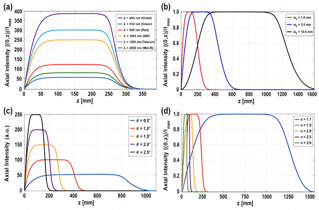
Figure 4 examines how the GPM-modified axial intensity varies when the principal design parameters are changed. In each subfigure, only one parameter is varied while the remaining parameters are kept fixed at the baseline values stated in the simulation caption. The curves are normalized to emphasize the shape and extent of the flat-top region rather than absolute power calibration.

Figure 4a shows the wavelength dependence for representative wavelengths from the visible to the mid-infrared. According to Equation (17), the required phase amplitude scales as $C_{\mathrm{o}\mathrm{p}\mathrm{t}}\propto 1/\lambda$ for fixed $w_0$, $n$, and $\theta$. This scaling does not mean that shorter wavelengths diffract more rapidly for a fixed waist; in fact, the Gaussian Rayleigh range $z_R=\pi w_0^2/\lambda$ increases as the wavelength decreases. The observed trend should therefore be interpreted as the combined effect of the conical phase slope, the GPM scaling, and the chosen normalization.

Figure 4b illustrates the influence of the input waist $w_0$. A larger input waist increases the available radial aperture that contributes to the conical interference process and increases the Rayleigh range quadratically. Consequently, the accessible flat-top length can be extended by beam expansion before the SLM, although this also requires an aperture large enough to avoid truncation.

Figure 4c shows the dependence on the axicon cone angle. The cone angle determines the transverse wave-vector component $k_t=k_0\left(n-1\right)\mathrm{t}\mathrm{a}\mathrm{n}\theta$ and hence the transverse size of the Bessel core. A larger cone angle gives a tighter central lobe but generally shortens the useful axial range because the contributing annuli are mapped to the axis over a shorter distance.

Figure 4d presents the effect of the axicon refractive index $n$. In the model, $n$ enters through the factor $\left(n-1\right)$ in the conical phase slope and in the GPM scaling. Increasing $n$ therefore strengthens the radial phase gradient for a fixed cone angle. In practical SLM implementations, this parameter is more naturally interpreted as an effective conical slope or grating period rather than a physical material index.

3.3. Physical Interpretation of Parametric Trends

The trends in Figure 4 can be understood from the stationary-phase relation in Equation (14). The GPM modifies both the saddle trajectory $r_s\left(z\right)$ and the curvature factor $S″\left(r_s;z\right)$. A flat-top axial response is obtained when the radial annuli of the input Gaussian beam are redistributed so that the natural Gaussian aperture decay is compensated by the phase-controlled annulus-to-axis mapping. Therefore, the decisive physical quantity is not simply the magnitude of the nonlinear phase, but the radial phase gradient and curvature that determine the saddle-point trajectory and its Jacobian.

This interpretation also explains why beam shaping must be optimized for the intended application. For TGV/TCV micromachining and light-sheet illumination, the goal is a long and smooth plateau with limited axial oscillation. For abrupt focusing, a localized axial peak may be desired instead. These are related through the same propagation theory, but they represent different design objectives and should not be treated as equivalent.

4. Bessel–Gaussian Beam Formulation with Non-GPM Function

This section clarifies the scope of the non-GPM phase study. The GPM design in Section 2 is intended primarily to flatten the axial intensity of a zero-order Bessel–Gaussian beam. By contrast, the cubic-exponential phase discussed here produces localized axial concentration and is better interpreted as a broader axial-intensity-engineering example, not as another flat-top solution.

For a Gaussian-apodized input carrying an azimuthal phase with topological charge $\mathcal{l}$, the phase-only mask may be written as

$${\Phi }_{\mathcal{l}}\left(r,\phi \right)=k_{t}r+\mathcal{l}\phi +C\mathrm{e}\mathrm{x}\mathrm{p}\left[-{\left({\displaystyle \frac{r}{w_0}}\right)}^3\right]$$

(18)

Here, $k_t=k_0\left(n-1\right)\mathrm{t}\mathrm{a}\mathrm{n}\theta$, $\mathcal{l}$ is an integer, and $C$ is the dimensionless amplitude of the cubic-exponential phase term. Under Fresnel propagation, angular integration gives a Bessel function of order $\mathcal{l}$. Apart from an overall phase factor, the propagated field can be written as

$$E_{\mathcal{l}}\left(\rho ,\phi ,z\right)\propto e^{j\mathcal{l}\phi }{\int }_0^{\mathrm{\infty }}r \mathrm{e}\mathrm{x}\mathrm{p}\left[-{\left({\displaystyle \frac{r}{w_0}}\right)}^2\right]J_{\mathcal{l}}\left({\displaystyle \frac{k_0\rho r}{z}}\right)\mathrm{e}\mathrm{x}\mathrm{p}\left[j{\Phi }_c\left(r;z\right)\right]\hspace{0.17em}dr$$

(19)

where the dimensionless radial phase is

$${\Phi }_c\left(r;z\right)={\displaystyle \frac{k_0{r}^2}{2z}}-k_{t}r-C\mathrm{e}\mathrm{x}\mathrm{p}\left[-{\left({\displaystyle \frac{r}{w_0}}\right)}^3\right]$$

(20)

The stationary radius $r_{*}$ is obtained from ${{\Phi }_c}^{\mathrm{\prime }}\left(r_{*};z\right)=0$ as follows:

$${\displaystyle \frac{k_0{r}_{*}}{z}}-k_t+{\displaystyle \frac{3C{r}_{*}^2}{w_0^3}}\mathrm{e}\mathrm{x}\mathrm{p}\left[-{\left({\displaystyle \frac{r_{*}}{w_0}}\right)}^3\right]=0$$

(21)

Equivalently, with $t={\left(r_{*}/w_0\right)}^3$,

$${\displaystyle \frac{k_0{w}_0}{z}}{t}^{1/3}-k_t+{\displaystyle \frac{3C}{w_0}}{t}^{2/3}{e}^{-t}=0$$

(22)

In numerical calculations, Equation (21) or Equation (22) should be solved directly because the diffraction term $k_0{r}_{*}/z$ is generally not negligible. If this term is neglected only as a large-$C$ estimate, the saddle can be approximated by

$$t\approx -{\displaystyle \frac{2}{3}}W\left[-{\displaystyle \frac{3}{2}}{\left({\displaystyle \frac{k_t{w}_0}{3C}}\right)}^{3/2}\right], r_{*}=w_0{t}^{1/3}$$

(23)

where $W\left(\cdot \right)$ is the Lambert $W$ function. This expression is useful only as an initial estimate for the numerical saddle search. The phase curvature required by the stationary-phase approximation is

$${\Phi }_c″\left(r_{*};z\right)={\displaystyle \frac{k_0}{z}}+{\displaystyle \frac{3C}{w_0^2}}{e}^{-t}\left(2t^{1/3}-3t^{4/3}\right)$$

(24)

For an isolated stationary point, the intensity can be expressed as

$$I_{\mathcal{l}}\left(\rho ,z\right)\approx I_{\mathrm{e}\mathrm{n}\mathrm{v}}^{\left(\mathcal{l}\right)}\left(z\right)J_{\mathcal{l}}^2\left({\displaystyle \frac{k_0{r}_{*}\rho }{z}}\right)$$

(25)

with the axial envelope,

$$I_{\mathrm{e}\mathrm{n}\mathrm{v}}^{\left(\mathcal{l}\right)}\left(z\right)={\left({\displaystyle \frac{2\pi }{\lambda z}}\right)}^2{\displaystyle \frac{2\pi r_{*}^2}{\left|{\Phi }_c″\left(r_{*};z\right)\right|}}\mathrm{e}\mathrm{x}\mathrm{p}\left[-2{\left({\displaystyle \frac{r_{*}}{w_0}}\right)}^2\right]$$

(26)

For the zero-order beam, $\mathcal{l}=0$ and $J_0\left(0\right)=1$, so the on-axis intensity is equal to the envelope in Equation (26). For higher-order vortex Bessel–Gaussian beams, $\mathcal{l}>0$ and $J_{\mathcal{l}}\left(0\right)=0$; therefore, the on-axis intensity vanishes by symmetry. In that case, the appropriate axial metric is not $I\left(0,z\right)$ but the maximum ring intensity or the annularly integrated power. For example,

$$I_{\mathrm{r}\mathrm{i}\mathrm{n}\mathrm{g}}\left(z\right)=\underset{\rho }{\mathrm{m}\mathrm{a}\mathrm{x}}\hspace{0.17em}{I}_{\mathcal{l}}\left(\rho ,z\right)$$

(27)

The cubic-exponential phase can generate abrupt axial localization in the linear scalar propagation model as shown in Figure 5. This localization may motivate further work on laser material processing or plasma-channel initiation, but the present calculations do not by themselves model nonlinear absorption, material modification, plasma formation, particle acceleration, or radiation yield.

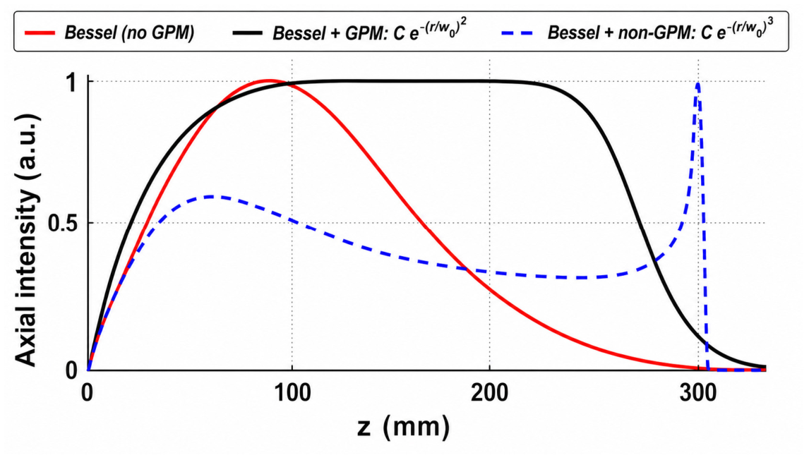
Figure 6 compares three zero-order axial propagation metrics: a conventional axicon-generated Bessel–Gaussian beam, the flat-top response obtained by adding GPM, and the localized response obtained with the cubic-exponential phase. The comparison clarifies that flat-top propagation and abrupt axial localization are distinct design objectives, even though both are produced by radial phase engineering.

5. Systematic Evaluation of Alternative Nonlinear Phase Functions for Flat-Top Bessel Beams

To clarify the novelty of the present manuscript relative to the previously reported GPM method, this section treats the GPM solution as a validated reference and evaluates whether other nonlinear radial phase profiles different than that presented in [24] which can reproduce the same flat-top axial transport law. In this study, the comparison includes logarithmic-transport (LTP), rational-quadratic (RQP), arctangent-squared (ATP), generalized exponential (GEP), hyperbolic-secant-squared (HSP), and Kaiser–Bessel phase profiles. All candidates are evaluated within the same Gaussian-apodized axicon model. The incident field immediately after the phase mask is written as

$$U_0\left(r\right)=A\mathrm{e}\mathrm{x}\mathrm{p}\left[-{\left({\displaystyle \frac{r}{w_0}}\right)}^2\right]\mathrm{e}\mathrm{x}\mathrm{p}\left[j{\Phi }_{\mathrm{t}\mathrm{o}\mathrm{t}}\left(r\right)\right]$$

(28)

where $A$ is the field-amplitude constant, $w_0$ is the Gaussian beam waist, and

$${\Phi }_{\mathrm{t}\mathrm{o}\mathrm{t}}\left(r\right)=-k_{t}r-{\varphi }_{\mathrm{N}\mathrm{L}}\left(r\right), k_t=k_0\left(n-1\right)\mathrm{t}\mathrm{a}\mathrm{n}\theta$$

(29)

Under paraxial Fresnel propagation, the radial phase used in the stationary-phase analysis is

$$\Psi \left(r;z\right)={\displaystyle \frac{k_0{r}^2}{2z}}-k_{t}r-{\varphi }_{\mathrm{N}\mathrm{L}}\left(r\right)$$

(30)

The saddle point is determined from

$${\Psi }^{\mathrm{\prime }}\left(r_s;z\right)={\displaystyle \frac{k_0{r}_s}{z}}-k_t-{{\varphi }_{\mathrm{N}\mathrm{L}}}^{\mathrm{\prime }}\left(r_s\right)=0$$

(31)

and the curvature is

$$\Psi ″\left(r_s;z\right)={\displaystyle \frac{k_0}{z}}-{\varphi }_{\mathrm{N}\mathrm{L}}″\left(r_s\right)$$

(32)

Substitution into the stationary-phase approximation gives the near-axis intensity

$$I\left(\rho ,z\right)\approx {\displaystyle \frac{8{\pi }^3{A}^2}{{\lambda }^2{z}^2}}{\displaystyle \frac{r_s^2\mathrm{e}\mathrm{x}\mathrm{p}\left[-2{\left(r_s/w_0\right)}^2\right]}{\left|\Psi ″\left(r_s;z\right)\right|}}{J}_0^2\left({\displaystyle \frac{k_0{r}_s\rho }{z}}\right)$$

(33)

and the on-axis intensity follows from $\rho =0$

$$I\left(0,z\right)\approx {\displaystyle \frac{8{\pi }^3{A}^2}{{\lambda }^2{z}^2}}{\displaystyle \frac{r_s^2\mathrm{e}\mathrm{x}\mathrm{p}\left[-2{\left(r_s/w_0\right)}^2\right]}{\left|\Psi ″\left(r_s;z\right)\right|}}$$

(34)

Equations (30)–(34) show that each phase function is governed primarily by its radial derivative and curvature, which control the saddle trajectory and the Jacobian factor. The optimization target was the normalized GPM flat-top reference curve, not an independently measured material-processing response. The root-mean-square error was calculated as

$$\mathrm{R}\mathrm{M}\mathrm{S}\left(\mathbf{p}\right)={\left[{\displaystyle \frac{1}{N}}{\displaystyle {\sum }_{i=1}^N}{\left(\tilde{I}\left(0,z_i;\mathbf{p}\right)-{\tilde{I}}_{\mathrm{r}\mathrm{e}\mathrm{f}}\left(z_i\right)\right)}^2\right]}^{1/2}$$

(35)

where

$$\tilde{I}\left(0,z_i;\mathbf{p}\right)={\displaystyle \frac{I\left(0,z_i;\mathbf{p}\right)}{\underset{z}{\mathrm{m}\mathrm{a}\mathrm{x}}I\left(0,z;\mathbf{p}\right)}}, {\tilde{I}}_{\mathrm{r}\mathrm{e}\mathrm{f}}\left(z_i\right)={\displaystyle \frac{I_{\mathrm{r}\mathrm{e}\mathrm{f}}\left(z_i\right)}{\underset{z}{\mathrm{m}\mathrm{a}\mathrm{x}}{I}_{\mathrm{r}\mathrm{e}\mathrm{f}}\left(z\right)}}$$

(36)

The coefficient of determination was evaluated as

$$R^2=1-{\displaystyle \frac{\sum _i{\left[\tilde{I}\left(0,z_i;\mathbf{p}\right)-{\tilde{I}}_{\mathrm{r}\mathrm{e}\mathrm{f}}\left(z_i\right)\right]}^2}{\sum _i{\left[{\tilde{I}}_{\mathrm{r}\mathrm{e}\mathrm{f}}\left(z_i\right)-⟨{\tilde{I}}_{\mathrm{r}\mathrm{e}\mathrm{f}}⟩\right]}^2}}$$

(37)

The optimization was carried out using the Nelder–Mead simplex method [36,37]. The propagation interval, sampling points, parameter bounds, free-parameter count, and initial values should be reported with the final MATLAB™ R2024b output so that the ranking can be reproduced. The optimization was performed over the axial range $z\in [0,\hspace{0.33em}0.25]$ m with 200 sampling points. For each candidate function, the adjustable parameters were bounded as follows: amplitude $C\in [10,\hspace{0.33em}150]$ (rad), radial shift $r_p\in [0,\hspace{0.33em}0.01]$ m, width $w_p\in [0.001,\hspace{0.33em}0.01]$ m, and shape exponents $m$ (generalized exponential phase) or $\beta$ (Kaiser–Bessel phase) $\in [1,\hspace{0.33em}10]$. Initial guesses were taken from the known Gaussian phase modulation parameters ($C\approx 75.8$, $r_p\approx 0.002$ m, $w_p\approx 0.00208$ m). The goal was to reproduce the normalized GPM reference curve (flat-top axial profile), not to independently maximize flatness. The Nelder–Mead simplex method (fminsearch) was used with a maximum of 180 iterations and a tolerance of ${10}^{-8}$ on parameters and ${10}^{-10}$ on the objective function. The goal was to minimize the RMS difference between the normalized axial intensity of each candidate and the normalized Gaussian phase reference curve, thereby assessing how faithfully each nonlinear phase reproduces the flat-top benchmark.

Figure 7 summarizes the analytical comparison. The generalized exponential phase gives the closest match to the GPM reference over the full flat-top region. The hyperbolic-secant-squared and rational-quadratic phases also retain the main plateau features; the black GPM reference curve is obscured because the other models overlap it closely, although with larger deviation near the leading or trailing edge. The logarithmic-transport and arctangent-squared phases decay too early, while the Kaiser–Bessel profile gives an intermediate result in the present implementation.

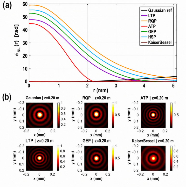
The transverse comparison in Figure 8 indicates that the best-performing candidates preserve a stable central lobe and annular ring structure close to the Gaussian reference. The result confirms that compact support alone is not sufficient; the radial phase-gradient structure must reproduce the saddle-point transport law that feeds the optical axis over the desired propagation interval. To facilitate further comparison,

Table 1. Analytical forms and comparative performance of the candidate nonlinear phase functions relative to the Gaussian benchmark.

Function	Nonlinear Phase ${\mathit{\varphi }}_{\mathbf{NL}}\left(\mathit{r}\right)$	Adjustable Parameters	Relative Performance	Principal Observation
Gaussian ref.	$C\mathrm{e}\mathrm{x}\mathrm{p}\left[-{\left({\displaystyle \frac{r-r_p}{w_p}}\right)}^2\right]$	$C,w_p,r_p$	Reference	Localized Gaussian correction producing the target flat-top profile.
LTP	$C\mathrm{l}\mathrm{n}\left[1+{\left({\displaystyle \frac{r-r_p}{w_p}}\right)}^2\right]$	$C,w_p,r_p$	Poor	Rapid initial rise but premature axial decay caused by an overly broad phase redistribution.
RQP	$C/{\left[1+{\left((r-r_p)/w_p\right)}^2\right]}^2$	$C,w_p,r_p$	Good	Maintains a broad plateau with moderate trailing-edge deviation and stable transverse structure.
ATP	$C {\mathrm{a}\mathrm{r}\mathrm{c}\mathrm{t}\mathrm{a}\mathrm{n}}^2\left({\displaystyle \frac{r-r_p}{w_p}}\right)$	$C,w_p,r_p$	Poor	Insufficient localization of the phase gradient leads to strong early decay.
GEP	$C \mathrm{e}\mathrm{x}\mathrm{p}\left[-{\left|{\displaystyle \frac{r-r_p}{w_p}}\right|}^m\right]$	$C,w_p,r_p,m$	Excellent	$C,w_p,m,r_p$
HSP	$C {\mathrm{s}\mathrm{e}\mathrm{c}\mathrm{h}}^2\left({\displaystyle \frac{r-r_p}{w_p}}\right)$	$C,w_p,r_p$	Good	Provides high-fidelity flat-top behavior with slightly larger deviation than GEP.
Kaiser–Bessel	$C\left[{\displaystyle \frac{I_0\left(\beta \sqrt{1-u^2}\right)-1}{I_0\left(\beta \right)-1}}\right],$ $\mathrm{where}\mathrm{u} ={\displaystyle \frac{r-r_p}{w_p}}, \left|u\right|\le 1,$	$C,w_p,r_p,\beta$	Poor

lists the analytical expressions and relative performance of the candidate nonlinear phase functions with respect to the Gaussian benchmark. The interpretive ranking, inferred from the analytical and BPM comparisons in Figure 7 and Figure 8, is explicitly summarized in

Table 2. Interpretive ranking inferred from the analytical and BPM comparisons in Figure 7 and Figure 8.

Rank	Function	Evidence from Figure 5 and Figure 6	Interpretation
1	GEP	Lowest RMS, R2 essentially equal to unity, intensity ratio closest to one, and stable Bessel-like transverse structure.	Best overall representation of the Gaussian benchmark and the most faithful flat-top solution among the tested families.
2	HSP	Low RMS, high R2, and near-unity intensity ratio over most of the plateau.	Strong practical alternative with smooth localization and good transverse stability.
3	RQP	Low RMS and high R2, with moderate deviation near the end of the plateau.	Useful secondary alternative when a rational phase law is preferred.
4	Kaiser–Bessel	Intermediate RMS and visibly broader transverse pattern at z = 0.2 m.	Compact support is attractive, but the present implementation does not reproduce the desired transport law with sufficient fidelity.
5	LTP	Large RMS and early axial decay despite a smooth phase profile.	Phase redistribution is too broad to maintain localized annular feeding.
6	ATP	Large RMS, low goodness of fit, and pronounced early decay.	Poor match to the Gaussian benchmark for sustained flat-top propagation.

.

6. Discussion: Advantages, Limitations, and Application Scope

This analysis clarifies the advantage of the engineered nonlinear phase masks over fixed axicon-based approaches. A conventional axicon maps the finite Gaussian aperture into a skewed axial envelope, whereas a programmable SLM phase can tune the radial phase gradient and curvature that determine the annulus-to-axis transport law. This permits dynamic selection between extended flat-top focusing, localized axial concentration, and alternative transverse structures without changing the optical hardware. The method is therefore attractive for applications in which the target depth, beam diameter, or axial energy distribution must be reconfigured.

At the same time, the application claims must be interpreted within the limits of the model. The present theory is a scalar, linear, paraxial propagation model. It predicts optical intensity distributions, but it does not simulate nonlinear absorption, heat accumulation, plasma formation, hydrodynamic channel evolution, electron acceleration, gamma-ray emission, or material removal. For TGV/TCV drilling, the flat-top Bessel–Gaussian field should be regarded as an optical input that may improve axial energy uniformity, while the final via shape depends on multiphoton absorption, avalanche ionization, thermal accumulation, chemical etching, and material response. Similarly, in high-energy and nuclear-related radiation applications, the structured optical field may be useful as a driver or waveguide-forming pulse, but particle-in-cell, plasma-fluid, or radiation-transport simulations are required before quantitative predictions can be made.

The experimental comparison in this work is also clarified using published work in [35]. The analytical and BPM calculations are generated in the present study, whereas the experimental data used for validation are adapted from earlier SLM-based measurements in Ref. [35].

7. Conclusions

This study presents a consistent framework for nonlinear phase engineering of flat-top Bessel–Gaussian beams. Starting from Fresnel diffraction theory, the full off-axis cylindrical propagation integral was written with the Bessel angular factor, and the stationary-phase derivation was reformulated using a single dimensionally consistent radial phase. The resulting expressions show that axial flattening is governed by the saddle-point trajectory and phase curvature, which together determine how optical energy is redistributed from the Gaussian input annuli to the propagation axis.

The main extension beyond the previously validated GPM method is the systematic comparison of alternative nonlinear radial phase profiles. The results show that high-performing candidates must reproduce the radial phase-gradient structure of the GPM benchmark, rather than only its phase amplitude or smoothness. Among the tested candidates, the generalized exponential phase gives the closest match to the GPM flat-top response, while the hyperbolic-secant-squared and rational-quadratic functions provide practical alternatives with good stability. The logarithmic-transport and arctangent-squared functions perform poorly, and the compact-support Kaiser–Bessel profile gives an intermediate response.

This research also separates flat-top Bessel-beam generation from abrupt axial localization. For zero-order beams, the on-axis intensity is a suitable metric. However, for higher-order vortex Bessel–Gaussian beams, the on-axis intensity vanishes by symmetry, so ring-maximum or annularly integrated intensity should be used. This correction resolves the ambiguity in the treatment of higher-order beams and clarifies the scope of the non-GPM cubic-exponential example. Overall, programmable nonlinear phase modulation provides a flexible route for tailoring the axial and transverse structure of femtosecond laser beams. The method is relevant to TGV/TCV micromachining, light-sheet illumination, and prospective high-intensity beam-delivery applications, but quantitative predictions for material processing or radiation generation require additional nonlinear propagation, material-response, or plasma-dynamics models.

References

1. Kim, J.; Kim, S.; Kim, B.; Choi, J.; Ahn, S. Study of Through Glass Via (TGV) Using Bessel Beam, Ultrashort Two-Pulses of Laser and Selective Chemical Etching. Micromachines 2023, 14, 1766. [Google Scholar] [CrossRef]
2. Rao, A.S.; Samanta, G.K. On-axis intensity modulation-free, segmented, zero-order Bessel beams with tunable ranges. Opt. Lett. 2018, 43, 3029–3032. [Google Scholar] [CrossRef]
3. Durnin, J. Exact solutions for nondiffracting beams I The scalar theory. J. Opt. Soc. Am. A 1987, 4, 651. [Google Scholar] [CrossRef]
4. Durnin, J.; Miceli, J.; Eberly, J.H. Diffraction-free beams. Phys. Rev. Lett. 1987, 58, 1499–1501. [Google Scholar] [CrossRef]
5. Mcgloin, D.; Dholakia, K. Bessel beams: Diffraction in a new light. Contemp. Phys. 2005, 46, 15–28. [Google Scholar] [CrossRef]
6. Zhai, Z.; Cheng, Z.; Lv, Q.; Wang, X. Tunable Axicons Generated by Spatial Light Modulator with High-Level Phase Computer-Generated Holograms. Appl. Sci. 2020, 10, 5127. [Google Scholar] [CrossRef]
7. Wu, P.; Sui, C.; Huang, W. Theoretical analysis of a quasi-Bessel beam for laser ablation. Photon. Res. 2014, 2, 82–86. [Google Scholar] [CrossRef]
8. Courvoisier, F.; Zhang, J.; Bhuyan, M.K.; Jacquot, M.; Dudley, J.M. Applications of femtosecond Bessel beams to laser ablation. Appl. Phys. A 2013, 112, 29–34. [Google Scholar] [CrossRef]
9. Du, T.; Wang, T.; Wu, F. Generation of three-dimensional optical bottle beams via focused non-diffracting Bessel beam using an axicon. Opt. Commun. 2014, 317, 24–28. [Google Scholar] [CrossRef]
10. Chremmos, I.; Efremidis, N.K.; Christodoulides, D.N. Pre-engineered abruptly autofocusing beams. Opt. Lett. 2011, 36, 1890–1892. [Google Scholar] [CrossRef]
11. Elsharkawi, A.S.A.; Lo, Y.-L. Correction of femtosecond laser asymmetric spot size for achieving uniform axial intensity in Bessel beam propagation via GPM. Opt. Lett. 2026, 51, 341–344. [Google Scholar] [CrossRef] [PubMed]
12. Gamaly, E.G. Femtosecond Laser-Matter Interaction: Theory, Experiments and Applications; Jenny Stanford Publishing: New York, NY, USA, 2011. [Google Scholar]
13. Keldysh, L.V. Ionization in the field of a strong electromagnetic wave. J. Exp. Theor. Phys. 1965, 20, 1307–1314. [Google Scholar]
14. Hafizi, B.; Esarey, E.; Sprangle, P. Laser-driven acceleration with Bessel beams. Phys. Rev. E 1997, 55, 3539–3545. [Google Scholar] [CrossRef]
15. Miao, B.; Feder, L.; Shrock, J.E.; Goffin, A.; Milchberg, H.M. Optical Guiding in Meter-Scale Plasma Waveguides. Phys. Rev. Lett. 2020, 125, 74801. [Google Scholar] [CrossRef]
16. Shrock, J.E.; Miao, B.; Feder, L.; Milchberg, H.M. Meter-scale plasma waveguides for multi-GeV laser wakefield acceleration. Phys. Plasmas 2022, 29, 73101. [Google Scholar] [CrossRef]
17. Miao, B.; Shrock, J.E.; Feder, L.; Hollinger, R.C.; Morrison, J.; Nedbailo, R.; Picksley, A.; Song, H.; Wang, S.; Rocca, J.J.; et al. Multi-GeV Electron Bunches from an All-Optical Laser Wakefield Accelerator. Phys. Rev. X 2022, 12, 31038. [Google Scholar] [CrossRef]
18. Wang, J.; Li, X.B.; Gan, L.F.; Xie, Y.; Zhong, C.L.; Zhou, C.T.; Zhu, S.P.; He, X.T.; Qiao, B. Generation of Intense Vortex Gamma Rays via Spin-to-Orbital Conversion of Angular Momentum in Relativistic Laser-Plasma Interactions. Phys. Rev. Appl. 2020, 14, 14094. [Google Scholar] [CrossRef]
19. Jiang, B.C.; Zhang, Q.L.; Chen, J.H.; Zhao, Z.T. Using a Bessel light beam as an ultrashort period helical undulator. Phys. Rev. Accel. Beams 2017, 20, 70701. [Google Scholar] [CrossRef]
20. Golub, I. Fresnel axicon. Opt. Lett. 2006, 31, 1890–1892. [Google Scholar] [CrossRef]
21. Courvoisier, F. Nonstandard Light for Ultrafast Laser Microstructuring and Nanostructuring. In Ultrafast Laser Nanostructuring: The Pursuit of Extreme Scales; Stoian, R., Bonse, J., Eds.; Springer International Publishing: Cham, Switzerland, 2023; pp. 581–621. [Google Scholar]
22. Brzobohatý, O.; Cižmár, T.; Zemánek, P. High quality quasi-Bessel beam generated by round-tip axicon. Opt. Express 2008, 16, 12688. [Google Scholar] [CrossRef]
23. Poujet, Y.; Roussey, M.; Salvi, J.; Baida, F.I.; Labeke, D.V. Super-transmission of light through subwavelength annular aperture arrays in metallic films: Spectral analysis and near-field optical images in the visible range. Photonics Nanostructures—Fundam. Appl. 2006, 4, 47–53. [Google Scholar] [CrossRef]
24. Elsharkawi, A.S.A.; Arafa, A.A.; Ahmed, A.A.M.; Chen, S.-Y.; Chang, C.-Y.; Lo, Y.-L. Beam shaping by nonlinear phase modulation for a femtosecond laser with a spatial light modulator. Opt. Lasers Eng. 2026, 201, 109713. [Google Scholar] [CrossRef]
25. Ouadghiri-Idrissi, I.; Giust, R.; Froehly, L.; Jacquot, M.; Furfaro, L.; Dudley, J.M.; Courvoisier, F. Arbitrary shaping of on-axis amplitude of femtosecond Bessel beams with a single phase-only spatial light modulator. Opt. Express 2016, 24, 11495–11504. [Google Scholar] [CrossRef]
26. Jaroszewicz, Z.; Sochacki, J.; Kołodziejczyk, A.; RafałStaronski, L. Apodized annular-aperture logarithmic axicon: Smoothness and uniformity of intensity distributions. Opt. Lett. 1993, 18, 1893–1895. [Google Scholar] [CrossRef] [PubMed]
27. Čižmár, T.; Dholakia, K. Tunable Bessel light modes: Engineering the axial propagation. Opt. Express 2009, 17, 15558–15570. [Google Scholar] [CrossRef]
28. Cao, S.; Ruan, Z.; Ren, W.; Qin, S.; Yin, X.; Liu, L.; Liang, Y.; Xu, H. Tailoring Perfect Optical Vortex Combs Based on Diffractive Neural Networks. Laser Photon. Rev. 2026, 20, e02383. [Google Scholar] [CrossRef]
29. Liang, Y.; Cao, S.; Liu, L.; Liu, F.; Yin, X.; Lv, P.; Zhang, Y.; Zou, Y.; Fang, L.; Zheng, S.; et al. Coherent detector for the non-separability measurement of vectorial structured light. Light Sci. Appl. 2025, 14, 343. [Google Scholar] [CrossRef]
30. Elsharkawi, A.S.A.; Tsai, I.-C.; Lin, X.-T.; Chang, C.-Y.; Lo, Y.-L. Bessel beam propagation using radial beam propagation method at different propagation scales. Opt. Express 2024, 32, 30242–30255. [Google Scholar] [CrossRef]
31. Elsharkawi, A.S.A.; Lo, Y.-L. Flattop axial Bessel beam propagation with analytical form of the phase retardation function. Opt. Lett. 2024, 49, 5403–5406. [Google Scholar] [CrossRef]
32. Saleh, B.E.A.; Teich, M.C. Fundamentals of Photonics; Wiley: New York, NY, USA, 2008; Volume 332. [Google Scholar]
33. Shaaban, A.; Du, Y.-C. An Optical Universal Plasmon-Based Biosensor for Virus Detection. J. Med. Biol. Eng. 2023, 43, 258–265. [Google Scholar] [CrossRef] [PubMed]
34. Shaaban, A.; Du, Y.-C.; Rabeh Gomaa, L. Transmissivity assessment of plasmonic-dielectric waveguide interconnects via modified FFT-BPM. Optik 2020, 208, 164143. [Google Scholar] [CrossRef]
35. Moon, J.B.; Lee, H.R.; Han, G.W.; Kim, J.W. Quasi-Bessel beam generation by a diffractive axicon with an exponential phase function. Opt. Laser Technol. 2024, 177, 111059. [Google Scholar] [CrossRef]
36. Olsson, D.M.; Nelson, L.S. The Nelder-Mead Simplex Procedure for Function Minimization. Technometrics 1975, 17, 45–51. [Google Scholar] [CrossRef]
37. Mcleod, R.R. Simplex of Nelder & Mead Simplex of Nelder & Mead Example. Computer 1965, 7, 308–313. [Google Scholar]
Figure 1. Propagated field of a Gaussian input modified only by a GPM for different values of the phase amplitude: (a) C = 0.9 , (b) C = 54 , and (c) C = 80 . The figure illustrates nonlinear phase-induced redistribution of the Gaussian field and should be interpreted separately from the axicon-assisted Bessel–Gaussian design.
Photonics 13 00538 g001
Figure 2. Bessel–Gaussian beam propagation calculated with the axicon phase and with the GPM-modified axicon phase. (a) Conventional axicon-generated Bessel–Gaussian beam described by Equation (11). (b) Flat-top Bessel–Gaussian beam generated by the phase in Equation (12) and evaluated using Equation (16).
Photonics 13 00538 g002
Figure 3. Validation of the GPM-modified zero-order Bessel–Gaussian beam. (a) Normalized on-axis intensity I ( 0 , z ) / I m a x from the stationary-phase model, BPM simulation, and experimental data adapted from Ref. [35]. (b) Normalized transverse intensity distribution at the middle of the flat-top region. (c) Longitudinal intensity map showing the extended axial plateau. Axes are given in millimeters or meters as labeled, and all intensities are normalized to the maximum value in each panel.
Photonics 13 00538 g003
Figure 4. Parametric dependence of the normalized axial intensity of the GPM-modified Bessel–Gaussian beam. (a) Wavelength λ , (b) input beam waist w 0 , (c) axicon cone angle θ , and (d) refractive index or effective axicon parameter n . In each panel, one parameter is varied while the others are fixed. Axial distances are labeled in meters, and intensities are normalized to the maximum value of the corresponding curve.
Photonics 13 00538 g004
Figure 5. Simulated propagation produced by the cubic-exponential non-GPM phase in Equation (19), with C = 54 . (a) Zero-order Bessel–Gaussian beam, for which the axial localization can be characterized by the on-axis intensity. (b) First-order Bessel–Gaussian beam, for which the on-axis intensity is zero and the ring-maximum or annularly integrated intensity should be used instead.
Photonics 13 00538 g005
Figure 6. Comparison of normalized axial metrics for three phase masks: pure axicon without GPM, axicon plus GPM, and axicon plus cubic-exponential non-GPM. The GPM profile is designed for flat-top propagation, whereas the cubic-exponential profile is designed for localized axial concentration.
Photonics 13 00538 g006
Figure 7. Analytical comparison of candidate nonlinear phase functions relative to the Gaussian benchmark: (a) normalized axial intensity, (b) RMS error, and (c) coefficient of determination R 2 . All curves are normalized to their own maxima and compared over the same axial design interval.
Photonics 13 00538 g007
Figure 8. Supporting phase and BPM evidence: (a) optimized nonlinear phase profiles and (b) normalized transverse intensity comparison at z = 0.2   m . The transverse comparison corresponds to Figure 7, and all intensity profiles are normalized for shape comparison.
Photonics 13 00538 g008