Modeling Diverse Hazard Shapes with the Power Length-Biased XLindley Distribution

Abstract

In many fields, including engineering, biology and economics, modeling and analyzing lifetime data is crucial for understanding the reliability and survival characteristics of systems and components. To address the limitations of existing lifetime distributions in capturing complex hazard rate behaviors, this article introduces a new and flexible two-parameter distribution, the power length-biased XLindley (PLXL) distribution. This distribution extends the XLindley distribution family by incorporating a power transformation applied to a length-biased variant, thereby enriching its structural flexibility. It can model a variety of hazard rate shapes, including increasing, decreasing, decreasing–increasing–decreasing and inverted bathtub forms, making it suitable for a range of real-world applications. We derive the statistical properties of the PLXL distribution and develop parameter estimation methods based on the maximum likelihood and the least squares approach. We conduct a comprehensive simulation study to evaluate the performance of the proposed estimators in terms of bias and mean squared error. The practical utility and superior adaptability of the PLXL distribution are demonstrated by applying it to real lifetime data sets.

1. Introduction

Modeling lifetime or survival data is pivotal in many scientific disciplines, especially reliability engineering, survival analysis, biostatistics, actuarial science, and risk assessment. Accurate characterization of time-to-event data is critical in all these domains for effective decision-making, forecasting, and risk evaluation. A fundamental aspect of any lifetime model is its hazard rate function (HRF), which quantifies the instantaneous failure or event occurrence rate at a given time, conditional on survival up to that time.

Classical models derived from the exponential, Weibull, and gamma distributions have long served as the foundation for lifetime data analysis. However, these models are limited in their ability to accommodate diverse hazard rate shapes. For instance, the exponential model assumes a constant hazard rate, while the Weibull and gamma models, although more flexible, can only represent monotonic hazard rates depending on the value of their shape parameters. These limitations make them inadequate for many real-world applications that exhibit non-monotonic or complex hazard rate patterns.

In practical settings, particularly in medical studies, biological experiments, and the reliability of mechanical systems, HRFs often exhibit non-monotonic patterns. For example, unimodal HRFs are frequently observed in medical studies [1]. In heart or kidney transplantation, the risk of failure typically increases during the initial adjustment period, peaks, and then decreases as the patient’s condition stabilizes. A similar pattern can be seen in the progression of certain diseases, where the risk of death rises to a maximum after a certain period and then gradually declines. This type of hazard rate reflects the common clinical scenario of early complications followed by improvement over time. In addition to unimodal hazard rates, HRFs can also exhibit a decreasing–increasing–decreasing pattern. For instance, data on the stress-rupture life of Kevlar 49/epoxy strands subjected to constant sustained pressure at 90% of the stress level until all strands fail have been found to follow a decreasing–increasing–decreasing HRF pattern [2]. Such complex hazard behaviors necessitate more flexible models capable of accurately capturing the full range of failure mechanisms and risk dynamics.

Over the past two decades, numerous generalized and modified distributions have been introduced to address various modeling needs. These include extensions and transformations of the exponential and Weibull distributions. In addition, several generalizations of the Lindley distribution [3] have been proposed, among which the power Lindley distribution [4], weighted Lindley distribution [5], and generalized Lindley distribution [6] are particularly popular. The power Lindley distribution can model decreasing, increasing, and decreasing–increasing–decreasing hazard rate shapes. The weighted Lindley distribution is suitable for modeling increasing and bathtub-shaped (i.e., decreasing then increasing) HRFs. The generalized Lindley distribution supports decreasing, increasing, and bathtub hazard shapes, depending on the parameter settings. While the corresponding models offer greater flexibility, several significant limitations remain. Firstly, many of these distributions can only model specific types of HRFs, most commonly monotonic or single-peak (bathtub or inverted bathtub) shapes, while more complex shapes, such as decreasing-increasing-decreasing, remain largely unexplored or inadequately modeled. While the power Lindley distribution can be used to model decreasing-increasing-decreasing shapes, it is not suitable for modeling unimodal hazard rate shapes. Even though the gamma, Weibull, Lindley, and power Lindley distributions do not inherently produce an increasing bathtub (IBT) HRF curve, their inverse variants (inverse gamma, inverse Weibull, inverse Lindley [7] and inverse power Lindley distributions [8]) can generate such a shape. However, a drawback is that these inverse versions are essentially constrained to that single non-monotonic form; they cannot flexibly represent increasing or decreasing hazard rates. Secondly, some proposed distributions involve more than two or three parameters, which increases computational complexity and poses challenges in parameter estimation, particularly when data are sparse or subject to censoring.

Furthermore, many existing flexible distributions lack closed-form expressions for key statistical functions, such as the cumulative distribution function (CDF), the reliability function, and the moments. This impedes their practical utility in analytical derivations, software implementation, and inferential procedures. Even when such distributions demonstrate promising theoretical flexibility, their HRF behavior is often not well characterized in the literature, creating a gap between theoretical development and practical interpretation.

In light of these challenges, the present study is motivated by the need to develop a parsimonious yet flexible distribution capable of modeling a wide range of hazard rate shapes, including decreasing, increasing, inverted bathtub, and decreasing-increasing-decreasing patterns. The aim is to create a new two-parameter distribution that can capture these diverse shapes while retaining analytical tractability and closed-form expressions for its probability density function (PDF) and distribution functions. It should also have interpretable parameterizations to facilitate theoretical understanding and practical application.

In terms of relevant references, the XLindley distribution was initially introduced by [9]. Subsequently, Metiri et al. [10] investigated its characterization through truncated moments, delving into its key properties and possible applications. Building on this foundation, Zinhom et al. [11] developed the wrapped XLindley distribution, while Etaga et al. [12] proposed a variation known as the double XLindley distribution. Beghriche et al. [13] introduced the inverse form of the XLindley distribution, further enriching the distribution’s structural flexibility and applicability. In further developments, MirMostafaee [14] introduced the exponentiated new XLindley distribution, which proves useful in modeling hazard rates with increasing or bathtub-shaped patterns. Gemeay et al. [15] considered the power of the new XLindley distribution, expanding the family further. Alghamdi et al. [16] introduced a discrete version called the Poisson Quasi-XLindley distribution, alongside a regression framework and empirical analysis. Another variant, the exponentiated XLindley distribution, was developed by [17] by incorporating an additional shape parameter to enhance flexibility. Musekwa and Makubate [18] extended this further by proposing the exponentiated generalized XLindley distribution, a three-parameter model capable of exhibiting diverse shapes such as positive or negative skewness, reverse-J, or symmetric forms. Using the alpha power transformation, Alsadat [19] created the truncated new XLindley distribution. Most recently, Kouadria and Zeghdoudi [20] investigated and analyzed various truncated versions of the new XLindley distribution.

In this article, we extend the XLindley distribution family by applying a power transformation to a length-biased variant, thereby enhancing its structural flexibility. The motivation for this work stems from both empirical and theoretical considerations. During our investigation of real data sets, such as those arising from medical survival times, engineering component lifetimes, and biological processes, it became evident that existing distributions frequently failed to provide a good fit or meaningful interpretation of the underlying hazard behavior. This inadequacy is particularly evident when the HRF is non-monotonic or exhibits multiple modes. From a theoretical perspective, the opportunity to expand the family of lifetime distributions by introducing a new distribution that encompasses existing distributions as specific or limiting cases, provides closed-form expressions, and allows for novel HRF shapes represents a valuable contribution to both statistical distribution theory and applied modeling.

In summary, the main contributions of this research are as follows:

• The development of a novel two-parameter lifetime distribution capable of modeling a wide range of complex hazard rate shapes, including decreasing, increasing, decreasing-increasing-decreasing, and inverted bathtub forms.
• Addressing a notable research gap by proposing a model that maintains analytical tractability while providing greater flexibility compared to existing models.
• A comprehensive mathematical treatment of the proposed model that encompasses its distributional properties, inferential methods, and applications to real-world data.
• Motivated by both theoretical considerations and practical limitations of existing models, the proposed distribution offers a valuable new tool for researchers and practitioners in fields where understanding time-to-event phenomena is essential.

The paper is organized as follows: Section 2 introduces the PLXL distribution and examines its statistical properties. Section 3 focuses on parameter estimation and presents a simulation study. Section 4 discusses the modeling of right-censored data using the proposed distribution. Section 5 illustrates practical applications of the distribution with real data sets. The article concludes with a summary and final remarks in Section 6.

2. PLXL Distribution and Its Statistical Properties

2.1. The PDF and Its Shape

The PDF of the PLXL distribution with parameters $\lambda$ and $\theta$ is given by

$$f\left(x\right)={\displaystyle \frac{\lambda {\theta }^3{x}^{2\lambda -1}}{{\theta }^2+2\theta +2}}\left(2+\theta +x^{\lambda }\right)e^{-\theta x^{\lambda }},x>0,\lambda >0,\theta >0.$$

It is obtained by taking the power transformation $Y^{1/\lambda }$, where Y denotes a length-biased XLindley random variable, i.e., with the following PDF:

$$f_0\left(x\right)={\displaystyle \frac{{\theta }^{3}x}{{\theta }^2+2\theta +2}}\left(2+\theta +x\right)e^{-\theta x},x>0,\theta >0.$$

The theorem below examines how the shape of the PDF of the PLXL distribution changes according to the values of the parameters.

Theorem 1.

The PDF of the PLXL distribution is as follows:

• decreasing if

  (a) 

  $0<\lambda <{\displaystyle \frac{1}{2}},\theta >0$,

  (b) 

  $\lambda ={\displaystyle \frac{1}{2}},\theta \ge \sqrt{2}-1$;

• unimodal if

  (a) 

  $\lambda >{\displaystyle \frac{1}{2}},\theta >0$,

  (b) 

  $\lambda ={\displaystyle \frac{1}{2}},0<\theta <\sqrt{2}-1$.

Proof. 

Differentiating the PDF $f\left(x\right)$ with respect to x gives

$$f^{\prime }\left(x\right)={\displaystyle \frac{\lambda {\theta }^3}{\theta +2}}{e}^{-\theta x^{\lambda }}{x}^{2\lambda -2}{\Psi }_1\left(x^{\lambda }\right),$$

where

$${\Psi }_1\left(y\right)=A_1{y}^2+B_{1}y+C_1,\mathrm{with}y=x^{\lambda },$$

and the coefficients are

$$A_1=-\lambda \theta ,B_1=3\lambda -\lambda \theta (\theta +2)-1,C_1=(2\lambda -1)(\theta +2).$$

Note that $f^{\prime }\left(x\right)$ and ${\Psi }_1\left(y\right)$ have the same sign.

The roots of the quadratic function ${\Psi }_1\left(y\right)=0$ are given by

$$y_1={\displaystyle \frac{B_1-\sqrt{B_1^2-4A_1{C}_1}}{-2A_1}},y_2={\displaystyle \frac{B_1+\sqrt{B_1^2-4A_1{C}_1}}{-2A_1}}.$$

Case (i): Decreasing PDF

(a)

If $0<\lambda \le {\displaystyle \frac{1}{3}},\theta >0$ or ${\displaystyle \frac{1}{3}}<\lambda <{\displaystyle \frac{1}{2}},\theta \ge -1+{\displaystyle \frac{\sqrt{2\lambda \sqrt{\lambda (1-2\lambda )}}}{\lambda }}$, then $A_1$, $B_1$, and $C_1$ are all negative. Hence, ${\Psi }_1\left(y\right)<0$ for all $y>0$ and the PDF is decreasing.

If ${\displaystyle \frac{1}{3}}<\lambda <{\displaystyle \frac{1}{2}},\theta <-1+{\displaystyle \frac{\sqrt{2\lambda \sqrt{\lambda (1-2\lambda )}}}{\lambda }}$, then ${\Psi }_1\left(0\right)<0$ and ${lim}_{y\to \infty }{\Psi }_1\left(y\right)=-\infty$, and the discriminant $B_1^2-4A_1{C}_1<0$, so the roots are complex. Hence, ${\Psi }_1\left(y\right)<0$ for all $y>0$, and the PDF is decreasing.

(b)

If $\lambda ={\displaystyle \frac{1}{2}},\theta \ge \sqrt{2}-1$, then $A_1$, $B_1$, and $C_1$ are negative, so the PDF is decreasing.

Case (ii): Unimodal PDF

(a)

If $\lambda >{\displaystyle \frac{1}{2}},\theta >0$, then $A_1<0$ and $C_1>0$. Regardless of the sign of $B_1$, the coefficients of ${\Psi }_1\left(y\right)$ exhibit exactly one sign change. By Descartes’ Rule of Signs, ${\Psi }_1\left(y\right)$ has exactly one positive root. Also, ${\Psi }_1\left(0\right)<0$ and ${lim}_{y\to \infty }{\Psi }_1\left(y\right)=\infty$. Therefore, ${\Psi }_1\left(y\right)$ changes sign once, and $f\left(x\right)$ is unimodal.

(b)

If $\lambda ={\displaystyle \frac{1}{2}},0<\theta <\sqrt{2}-1$, then ${\Psi }_1\left(0\right)=0$, ${lim}_{y\to \infty }{\Psi }_1\left(y\right)=-\infty$, and ${\Psi }_1\left(y\right)$ has one positive real root. Hence, the PDF is unimodal.

   □

Figure 1 illustrates both the decreasing and unimodal shapes of the PDF of the PLXL distribution.

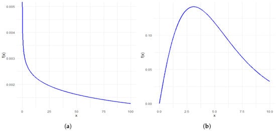
Figure 1. PDF plots of the PLXL distribution for (a) $\lambda$ = 0.4, $\theta$ = 0.2, (b) $\lambda$ = 1, $\theta$ = 0.5.

The mode of the PLXL distribution can be determined using Theorem 1, as shown below.

• The mode is at zero if

  $$0<\lambda <{\displaystyle \frac{1}{2}},\theta >0\mathrm{or}\lambda ={\displaystyle \frac{1}{2}},\theta \ge \sqrt{2}-1.$$
• If $\lambda >{\displaystyle \frac{1}{2}},\theta >0$, the mode $x_m$ is

  $$x_m={\left({\displaystyle \frac{3\lambda -\lambda \theta {(\theta +2)}^{-1}-\sqrt{{\left(3\lambda -\lambda \theta {(\theta +2)}^{-1}\right)}^2+4\lambda \theta (2\lambda -1)(\theta +2)}}{2\lambda \theta }}\right)}^{1/\lambda }.$$
• If $\lambda ={\displaystyle \frac{1}{2}},\theta >0$, the mode is

  $$x_m={\left({\displaystyle \frac{3\lambda -\lambda \theta {(\theta +2)}^{-1}}{\lambda \theta }}\right)}^{1/\lambda }.$$

The survival function (SF) of the PLXL distribution is given by

$$S\left(x\right)={\displaystyle \frac{e^{-\theta x^{\lambda }}}{{\theta }^2+2\theta +2}}\left({\theta }^2{x}^{2\lambda }+({\theta }^3+2{\theta }^2+2\theta )x^{\lambda }+{\theta }^2+2\theta +2\right),x>0.$$

The CDF is

$$F\left(x\right)=1-{\displaystyle \frac{e^{-\theta x^{\lambda }}}{{\theta }^2+2\theta +2}}\left({\theta }^2{x}^{2\lambda }+({\theta }^3+2{\theta }^2+2\theta )x^{\lambda }+{\theta }^2+2\theta +2\right),x>0.$$

2.2. The HRF and Its Shapes

The HRF of the PLXL is given by

$$h\left(x\right)={\displaystyle \frac{\lambda {\theta }^3{x}^{2\lambda -1}(2+\theta +x^{\lambda })}{{\theta }^2{x}^{2\lambda }+({\theta }^3+2{\theta }^2+2\theta )x^{\lambda }+({\theta }^2+2\theta +2)}}.$$

As with the PDF, we discuss the shape of the HRF for various parameter values. It should be noted that the SF, CDF and HRF all have a closed-form expression. The closed-form expression of the SF will be useful for modeling censored data.

Theorem 2.

If $\lambda \ge 1,\theta >0$, then the HRF is increasing.

If $1/2<\lambda <1,\theta >0$, or $\lambda =1/2,0<\theta <\sqrt{2}-1$, then the HRF is IBT shaped.

If $0<\lambda \le 1/3,\theta >0$, or $1/3<\lambda <1/2,\theta \ge \sqrt{2\lambda /(1-\lambda )}-1$, or $\lambda =1/2,\theta \ge \sqrt{2}-1$, then the HRF is decreasing.

If $1/3<\lambda <1/2,0<\theta <\sqrt{2\lambda /(1-\lambda )}-1$, then the HRF is as follows:

• Decreasing if ${\Psi }_2\left(y_0\right)<0$.
• Non-increasing if ${\Psi }_2\left(y_0\right)=0$.
• Decreasing-increasing-decreasing if ${\Psi }_2\left(y_0\right)>0$.

Additionally,

$${\Psi }_2\left(y\right)=A{y}^3+B{y}^2+Cy+D,$$

with

$$A_2=(\lambda -1){\theta }^2,B_2=2\theta ((\lambda -1)\theta (\theta +2)+2\lambda -1),$$

$$C_2=({\theta }^2+2\theta +2)((\lambda -1)\theta (\theta +2)+3\lambda -1),D_2=(2\lambda -1)({\theta }^3+4{\theta }^2+6\theta +4),$$

and

$$y_0={\displaystyle \frac{B_2+\sqrt{B_2^2-4A_2{C}_2}}{-2A_2}}.$$

Proof. 

The first derivative of HRF is

$$h^{\prime }\left(x\right)={\displaystyle \frac{\lambda {\theta }^3{x}^{2\lambda -2}{\Psi }_2\left(x^{\lambda }\right)}{{\left({\theta }^2{x}^{2\lambda }+({\theta }^3+2{\theta }^2+2\theta )x^{\lambda }+({\theta }^2+2\theta +2)\right)}^2}}.$$

One can see that $h^{\prime }(·)$ and ${\Psi }_2(·)$ have the same signs. If $\lambda \ge 1,\theta >0$, then $A_2,B_2,C_2$ and $D_2$ are positive and hence this case corresponds to an increasing hazard rate.

If $1/2<\lambda <1,\theta >0$, then $A_2$ is negative and $D_2$ is positive. Note that $C_2>B_2$; if $C_2$ is negative, then $B_2$ is also negative. Thus, we cannot have a scenario where $C_2$ is negative and $B_2$ is positive. Hence, various possibilities of signs of $A_2,B_2,C_2$ and $D_2$ are as follows:

(i)

$-,-,+,+$.

(ii)

$-,+,+,+$.

(iii)

$-,-,-,+$.

Observe that the number of sign changes in the coefficients of ${\Psi }_2\left(y\right)$ is one. Hence, using Descartes’ Rule of Signs (see [21]), there exists one positive root of equation ${\Psi }_2\left(y\right)=0$. We also have ${\Psi }_2\left(0\right)>0,{lim}_{y\to \infty }{\Psi }_2\left(y\right)=-\infty$. Therefore ${\Psi }_2(·)$ changes the sign from positive to negative one time. Hence ${\Psi }_2(·)$ is unimodal.

If $\lambda =1/2,\theta \ge \sqrt{2}-1$, then we have ${\Psi }_2\left(0\right)=0,{lim}_{y\to \infty }{\Psi }_2\left(y\right)=-\infty$, and also there exists one positive root. Hence this case corresponds to the IBT shape.

Note that if $0<\lambda \le 1/3,\theta >0$ or $1/3<\lambda <1/2,\theta \ge \sqrt{2\lambda /(1-\lambda )}-1$, then $A_2,B_2,C_2$ and $D_2$ are negative. $D_2$ is zero and $A_2,B_2,$ and $C_2$ are negative if $\lambda =1/2,\theta \ge \sqrt{2}-1$. Therefore, these cases correspond to a decreasing hazard rate.

If $1/3<\lambda <1/2,0<\theta <\sqrt{2\lambda /(1-\lambda )}-1$, then the cubic equation ${\Psi }_2\left(y\right)$ changes the direction one time at

$$y=y_0={\displaystyle \frac{B_2+\sqrt{B_2^2-4A_2{C}_2}}{-2A_2}}$$

over the positive real line. Since ${\Psi }_2\left(0\right)<0,{lim}_{y\to \infty }{\Psi }_2\left(y\right)=-\infty$, over the positive real line ${\Psi }_2(·)$ attains maximum value at

$$y={\displaystyle \frac{B_2+\sqrt{B_2^2-4A_2{C}_2}}{-2A_2}}.$$

• If ${\Psi }_2\left(y_0\right)<0$, then ${\Psi }_2\left(y\right)<0$ for all positive y, and hence the HRF is decreasing.
• If ${\Psi }_2\left(y_0\right)=0$, then the HRF is non-increasing since ${\Psi }_2(·)$ is negative for all positive y except at $y_0$.
• If ${\Psi }_2\left(y_0\right)>0$, then there should be two positive roots. Since ${\Psi }_2(·)$ changes direction one time with ${\Psi }_2\left(0\right)<0,{lim}_{y\to \infty }{\Psi }_2\left(y\right)=-\infty$, we must have decreasing-increasing-decreasing shape for the hazard rate.

   □

The classification of HRF shapes for the PLXL distribution under different parameter regimes is considered in Figure 2. The various shapes of HRF of the PLXL distribution are displayed in Figure 3.

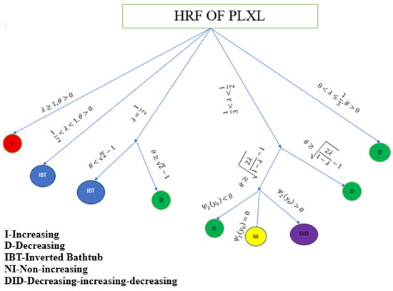
Figure 2. Classification of the HRF shapes for the PLXL distribution under different parameter regimes.

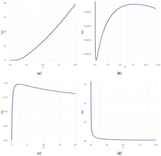
Figure 3. HRF plots of the PLXL distribution for (a) $\lambda$ = 2.5, $\theta$ = 0.5, (b) $\lambda$ = 0.48, $\theta$ = 0.2, (c) $\lambda$ = 0.8, $\theta$ = 2, (d) $\lambda$ = 0.2, $\theta$ = 1.

2.3. Change Point of the HRF

In the previous subsection, we proved that the HRF of the PLXL distribution can be IBT-shaped and non-monotonic, with a decreasing-increasing-decreasing pattern. Therefore, it is essential to investigate the change point of the HRF. It should be noted that at the change point of the HRF, its first derivative is zero. In order to identify this change point, it is first necessary to determine the positive root of the following cubic equation:

$${\Psi }_2\left(y\right)=A{y}^3+B{y}^2+Cy+D=0.$$

If $y^{*}$ is the positive root of ${\Psi }_2\left(y\right)=0$, then the change point of the HRF is ${\left(y^{*}\right)}^{1/\lambda }$.

The change points of some of the selected parameters are given in Table 1. The polyroot() function in R software [22] is used to obtain the roots of a cubic equation.

Table 1. The change points of the HRF of the PLXL distribution for some selected parameter values.

Parameters ($\mathit{\lambda },\mathit{\theta }$)	Number of Change Points of the HRF	Change Points of the HRF
(0.48, 0.2)	2	0.2038 and 7.7224
(0.8, 2)	1	2.24614
(0.75, 0.1)	1	210.48
(0.45, 0.1)	2	0.9706 and 50.3780
(0.9, 0.5)	1	49.27

Some lifetime data related to diseases show an inverted bathtub curve for the hazard rate. Therefore, it is important to identify the change point of the hazard rate. As can be seen from Table 1, there are parameters for which the PLXL distribution can exhibit a decreasing-increasing-decreasing shape for the HRF.

2.4. Moments of the PLXL Distribution

Let us now discuss the moments of the PLXL distribution. After some developments, the raw moment of a random variable X with the PLXL distribution is given by

$${\mu }_r^{\prime }=E\left(X^r\right)={\displaystyle \frac{\Gamma \left(\frac{2\lambda +r}{\lambda }\right)\left(r+({\theta }^2+2\theta +2)\lambda \right)}{\lambda {\theta }^{r/\lambda }({\theta }^2+2\theta +2)}},$$

(1)

where $\Gamma \left(a\right)={\int }_0^{\infty }{x}^{a-1}{e}^{-x}dx$ is the standard gamma function. When $r=1$ in (1), we obtain the mean, which is given by

$$E\left(X\right)={\displaystyle \frac{\Gamma \left(\frac{2\lambda +1}{\lambda }\right)\left(1+({\theta }^2+2\theta +2)\lambda \right)}{\lambda {\theta }^{1/\lambda }({\theta }^2+2\theta +2)}}.$$

Similarly, we can find the variance, which is as follows:

$$\begin{array}{cc}\hfill V\left(X\right)& ={\displaystyle \frac{\Gamma \left(\frac{2\lambda +2}{\lambda }\right)\left(2+({\theta }^2+2\theta +2)\lambda \right)}{\lambda {\theta }^{2/\lambda }({\theta }^2+2\theta +2)}}\hfill \\ \hfill & -{\left({\displaystyle \frac{\Gamma \left(\frac{2\lambda +1}{\lambda }\right)\left(1+({\theta }^2+2\theta +2)\lambda \right)}{\lambda {\theta }^{1/\lambda }({\theta }^2+2\theta +2)}}\right)}^2.\hfill \end{array}$$

These moment measures in close form are an advantage of the PLXL distribution.

3. Estimation and Simulation

The model parameters are estimated using maximum likelihood (ML) and least square (LS) techniques. The mean square error (MSE) of the estimators obtained using these two techniques is then computed to compare them.

3.1. ML Estimation

For a random sample $x_1,x_2,\dots ,x_n$ from the PLXL distribution, the log-likelihood function $lnL$ is given by

$$lnL=nln\left({\displaystyle \frac{\lambda {\theta }^3}{{\theta }^2+2\theta +2}}\right)-\theta \sum _{i=1}^n{x}_i^{\lambda }+\sum _{i=1}^{n}ln(2+\theta +x_i^{\lambda }),$$

The score functions are

$$\begin{array}{cc}\hfill {\displaystyle \frac{\partial lnL}{\partial \lambda }}& ={\displaystyle \frac{n}{\lambda }}+2\sum _{i=1}^{n}ln\left(x_i\right)-\theta \sum _{i=1}^n{x}_i^{\lambda }ln\left(x_i\right)+\sum _{i=1}^n{\displaystyle \frac{x_i^{\lambda }ln\left(x_i\right)}{2+\theta +x_i^{\lambda }}}=0\hfill \end{array}$$

(2)

and

$$\begin{array}{cc}\hfill {\displaystyle \frac{\partial lnL}{\partial \theta }}& ={\displaystyle \frac{3n}{\theta }}-{\displaystyle \frac{2n(\theta +1)}{{\theta }^2+2\theta +2}}+\sum _{i=1}^n{\displaystyle \frac{1}{2+\theta +x_i^{\lambda }}}-\sum _{i=1}^n{x}_i^{\lambda }=0.\hfill \end{array}$$

(3)

The ML estimators (MLE) of $\lambda$ and $\theta$ are solutions of the non-linear Equations (2) and (3).

3.2. LS Estimation

Here, a regression-based method estimator, proposed by [23], is used. Let $x_1,x_2,\dots ,x_n$ be a random sample from the proposed distribution. Let $x_{\left(i\right)}$, $i=1,2,\dots ,n$ be the ordered sample and $X_{\left(i\right)}$, $i=1,2,\dots ,n$ be the corresponding random variables. Then,

$$E\left(F\left(X_{\left(i\right)}\right)\right)={\displaystyle \frac{i}{n+1}},$$

see [24]. Then least square estimators (LSE) are obtained by minimizing

$$Q(\lambda ,\theta )=\sum _{i=1}^n{\left(F\left(x_{\left(i\right)}\right)-{\displaystyle \frac{i}{n+1}}\right)}^2.$$

Hence LSE are those values of $\lambda$ and $\theta$ which minimize

$$Q(\lambda ,\theta )=\sum _{i=1}^n{\left(1-{\displaystyle \frac{e^{-\theta x_{\left(i\right)}^{\lambda }}}{{\theta }^2+2\theta +2}}\left({\theta }^2{x}_{\left(i\right)}^{2\lambda }+({\theta }^3+2{\theta }^2+2\theta )x_{\left(i\right)}^{\lambda }+({\theta }^2+2\theta +2)\right)-{\displaystyle \frac{i}{n+1}}\right)}^2.$$

It is difficult to obtain a closed-form expression for $\lambda$ and $\theta$. For optimization, the optim command in R software is used.

3.3. Generating Random Observations

It is interesting to note that some of the well-known generalized Lindley distributions are obtained from the mixture of generalized gamma ($GG$) distribution. A three-parameter $GG$ distribution has the following PDF:

$$f_{GG}\left(x\right)={\displaystyle \frac{\alpha {\beta }^{\nu }{x}^{\alpha \nu -1}}{\Gamma \left(\nu \right)}}{e}^{-\beta x^{\alpha }},\alpha >0,\nu >0,\beta >0,x>0.$$

The GG distribution with shape parameters $\nu ,\alpha$ and scale parameter $\beta$ is denoted by $GG(\nu ,\alpha ,\beta )$.

Theorem 3.

The PDF of the PLXL distribution can be represented as

$$f\left(x\right)=p{f}_1\left(x\right)+(1-p)f_2\left(x\right),$$

where $f_1(·)$ is the PDF of the $GG(2,\lambda ,\theta )$ and $f_2(·)$ is the PDF of the $GG(3,\lambda ,\theta )$, and the mixing proportion is

$$p={\displaystyle \frac{{\theta }^2+2\theta }{{\theta }^2+2\theta +2}}.$$

To generate the observation from PLXL distribution, we consider the following steps:

• Generate observations $z_i^{\prime }$ and $z_i^{\prime \prime }$, $i=1,2,\dots ,n$, from the GG distributions: $GG(2,\lambda ,\theta )$ and $GG(3,\lambda ,\theta )$, respectively.
• Generate observations $u_i$ from the uniform distribution over (0, 1).
• If $u_i\le {\displaystyle \frac{{\theta }^2+2\theta }{{\theta }^2+2\theta +2}}$, set $x_i=z_i^{\prime }$; else, set $x_i=z_i^{\prime \prime }$.

3.4. Comparison of the ML and LS Estimations Using Simulated Observations

To compare the performance of the MLE and LSE, random observations are generated from the PLXL distribution using the algorithm mentioned above. The simulation was repeated $N=10,000$ times with sample sizes $n=20,50,100,150$ for different values of $\lambda$ and $\theta$.

The MSE for the parameter $\lambda$ is given by

$$\mathrm{MSE}\left(\lambda \right)={\displaystyle \frac{1}{N}}\sum _{i=1}^N{({\widehat{\lambda }}_i-\lambda )}^2,$$

where ${\widehat{\lambda }}_i$ denotes the estimate of $\lambda$ constructed from the i-th sample.

Similarly, the MSE of $\theta$ can be obtained. Along with the MSEs, we also compute the average estimates (AEs) for the parameters $\lambda$ and $\theta$. The AEs and MSEs for the MLEs and LSEs of $\lambda$ and $\theta$ are computed and compared in Table 2 and Table 3, respectively.

Table 2. MSEs and AEs for the parameter $\theta$ using both the techniques (MLE and LSE).

$\mathit{\lambda }$	$\mathit{\theta }$	n	AE (MLE)	AE (LSE)	MSE (MLE)	MSE (LSE)
0.5	0.8	20	0.5111	0.5924	0.0026	0.7022
		50	0.5044	0.5020	0.0008	0.0018
		100	0.5023	0.5011	0.0004	0.0009
		150	0.5016	0.5007	0.0003	0.0006
0.6	1.0	20	0.6167	0.6227	0.0052	0.1348
		50	0.6066	0.6026	0.0017	0.0041
		100	0.6033	0.6016	0.0008	0.0019
		150	0.6023	0.6012	0.0005	0.0012
1.0	0.5	20	1.0150	1.0587	0.0057	0.4178
		50	1.0061	1.0020	0.0020	0.0035
		100	1.0027	1.0014	0.0010	0.0016
		150	1.0018	1.0005	0.0006	0.0011
2.0	1.5	20	2.0768	1.9323	0.1027	0.1940
		50	2.0325	1.9758	0.0346	0.0713
		100	2.0148	1.9882	0.0156	0.0351
		150	2.0099	1.9938	0.0104	0.0229

Table 3. MSEs and AEs for the parameter $\theta$ using both the techniques (MLE and LSE).

$\mathit{\lambda }$	$\mathit{\theta }$	n	AE (MLE)	AE (LSE)	MSE (MLE)	MSE (LSE)
0.5	0.8	20	0.8140	0.8075	0.0129	0.0148
		50	0.8067	0.8046	0.0046	0.0054
		100	0.8032	0.8024	0.0023	0.0027
		150	0.8024	0.8017	0.0015	0.0018
0.6	1.0	20	1.0187	1.0103	0.0207	0.0237
		50	1.0084	1.0057	0.0075	0.0088
		100	1.0045	1.0035	0.0037	0.0043
		150	1.0035	1.0027	0.0024	0.0028
1.0	0.5	20	0.5095	0.5043	0.0046	0.0054
		50	0.5037	0.5022	0.0017	0.0020
		100	0.5016	0.5015	0.0008	0.0009
		150	0.5012	0.5007	0.0006	0.0007
2.0	1.5	20	1.5344	1.5174	0.0479	0.0556
		50	1.5121	1.5075	0.0183	0.0208
		100	1.5071	1.5042	0.0088	0.0102
		150	1.5047	1.5047	0.0058	0.0068

The following observations can be drawn from these tables:

• In all the cases, the MSEs of the MLEs and LSEs of both $\lambda$ and $\theta$ decrease as sample size increases. This also indicates that the estimators $\widehat{\lambda }$ and $\widehat{\theta }$ are consistent.
• In all the cases, the MSEs of the MLEs of both $\lambda$ and $\theta$ are lesser than the MSEs of LSEs of $\lambda$ and $\theta$. This shows that the MLEs perform better than the LSEs.
• As sample size increases, the differences in MSE of MLEs and LSEs decrease, indicating that for large sample sizes, the MLEs and LSEs are almost equally efficient.

4. Modeling Right-Censored Data

In survival analysis, right-censored data occur when the event of interest has not been observed within the study period. For instance, in a clinical trial, a patient might leave the study before experiencing the event (e.g., relapse), or the study might end before the event occurs. In such cases, we know that the event time exceeds a certain value but don’t know the exact time.

Let $x_1,x_2,\dots ,x_n$ represent a random sample from the PLXL distribution. For each observation $x_i$, let ${\delta }_i$ be the censoring indicator, defined as

$${\delta }_i=\left\{\begin{array}{cc}1\hfill & \mathrm{if}\mathrm{the}i-\mathrm{th}\mathrm{observation}\mathrm{is}\mathrm{uncensored}\hfill \\ 0\hfill & \mathrm{if}\mathrm{the}i-\mathrm{th}\mathrm{observation}\mathrm{is}\mathrm{censored}\hfill \end{array}\right.$$

The likelihood function L is given by

$$L=\prod _{i=1}^n{\left[f\left(x_i\right)\right]}^{{\delta }_i}{\left[S\left(x_i\right)\right]}^{1-{\delta }_i}.$$

Accordingly, the log-likelihood function is

$$lnL=\sum _{i=1}^n\left[{\delta }_{i}lnf\left(x_i\right)+(1-{\delta }_i)lnS\left(x_i\right)\right].$$

To estimate the parameters $\lambda$ and $\theta$, we maximize the log-likelihood function with respect to these parameters. Given the complexity of the log-likelihood function, analytical solutions may not be feasible. Therefore, numerical optimization techniques are employed to obtain the maximum likelihood estimates (MLEs).

5. Real-Life Application

In this section, we explore the practical applications of the proposed lifetime model, emphasizing its relevance in real-world scenarios. Understanding the distribution of lifetimes is crucial in various fields, including medical research and reliability engineering. We address both censored and uncensored data sets, providing a comprehensive framework for analyzing lifetime data.

5.1. Modelling Uncensored Data

In this subsection, we focus on analysing lifetime data where all events are fully observed, without any censoring. Such data provide complete information about the time to event. We consider two such data sets. The first data set encompasses COVID-19 vaccination rates across 46 Southern African nations [25], detailing the number of individuals who have received full vaccinations per 100 people. The second data set investigates the failure stresses (in GPa) of 20 mm-long single carbon fibers [4], providing insights into their mechanical properties. The data sets are given below:

• Data set 1 (Vaccination rates):
  0.042, 0.205, 0.285, 0.319, 0.464, 0.550, 0.889, 0.895, 0.939, 0.986, 1.000, 1.088, 1.212, 1.244, 1.450, 1.593, 1.844, 2.039, 2.157, 2.167, 2.334, 2.440, 2.657, 3.685, 3.879, 4.493, 4.800, 4.944, 5.155, 5.674, 7.602, 10.004, 12.238, 12.520, 12.553, 13.063, 15.105, 15.229, 15.629, 15.848, 18.641, 18.940, 29.885, 58.162, 61.838, 72.286.
• Data set 2 (Carbon fiber stress):
  1.312, 1.314, 1.479, 1.552, 1.700, 1.803, 1.861, 1.865, 1.944, 1.958, 1.966, 1.997, 2.006, 2.021, 2.027, 2.055, 2.063, 2.098, 2.140, 2.179, 2.224, 2.240, 2.253, 2.270, 2.272, 2.274, 2.301, 2.301, 2.359, 2.382, 2.382, 2.426, 2.434, 2.435, 2.478, 2.490, 2.511, 2.514, 2.535, 2.554, 2.566, 2.570, 2.586, 2.629, 2.633, 2.642, 2.648, 2.684, 2.697, 2.726, 2.770, 2.773, 2.800, 2.809, 2.818, 2.821, 2.848, 2.880, 2.954, 3.012, 3.067, 3.084, 3.090, 3.096, 3.128, 3.233, 3.433, 3.585, 3.585.

To verify the shape of the HRF, we used the total time on test (TTT) plot. For details about the TTT plot and its construction, we refer to [26]. A data set is said to have an IBT shaped HRF if the TTT plot is convex followed by concave. A concave–convex shape suggests a bathtub HRF. If the TTT plot is purely convex, it indicates a decreasing HRF, while a concave TTT plot indicates an increasing HRF.

Figure 4 shows the TTT plots along with bootstrap band for data sets 1 and 2. It is evident from the Figure 4 that the HRF is decreasing for data set 1, and increasing for data set 2.

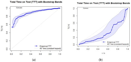
Figure 4. TTT plots of (a) data set 1, (b) data set 2.

In addition to the proposed PLXL distribution, several well-known two-parameter lifetime distributions capable of modeling HRFs with both increasing and decreasing shapes were also fitted to data sets 1 and 2. The considered competing distributions are briefly described below:

• Gamma distribution:

  $$f_G\left(x\right)={\displaystyle \frac{{\theta }^{\lambda }}{\Gamma \left(\lambda \right)}}{e}^{-\theta x}{x}^{\lambda -1},x>0,\lambda >0,\theta >0.$$
• Weibull distribution:

  $$f_W\left(x\right)=\lambda \theta x^{\lambda -1}{e}^{-\theta x^{\lambda }},x>0,\lambda >0,\theta >0.$$
• Exponentiated Exponential (EE) [27] distribution:

  $$f_{EE}\left(x\right)=\lambda \theta {\left(1-e^{-\theta x}\right)}^{\lambda -1}{e}^{-\theta x},x>0,\lambda >0,\theta >0.$$
• Generalized Lindley (GL) [6] distribution:

  $$f_{GL}\left(x\right)={\displaystyle \frac{\lambda {\theta }^2}{\theta +1}}(1+x){\left(1-{\displaystyle \frac{1+\theta +\theta x}{1+\theta }}{e}^{-\theta x}\right)}^{\lambda -1}{e}^{-\theta x},x>0,\lambda >0,\theta >0.$$
• Power Lindley (PL) [4] distribution:

  $$f_{PL}\left(x\right)={\displaystyle \frac{\lambda {\theta }^2}{\theta +1}}(1+x^{\lambda })x^{\lambda -1}{e}^{-\theta x^{\lambda }},x>0,\lambda >0,\theta >0.$$
• Power XLindley (PXL) distribution:

  $$f_{PXL}\left(x\right)={\displaystyle \frac{\lambda {\theta }^2{x}^{\lambda -1}}{{(1+\theta )}^2}}\left(2+\theta +x^{\lambda }\right)e^{-\theta x^{\lambda }},x>0,\lambda >0,\theta >0.$$

Table 4 and Table 5 present the MLEs of the model parameters along with the standard error (SE), Kolmogorov-Smirnov (K-S) test statistic, Anderson-Darling (AD) statistic, Cramér-von Mises (CvM) statistic along with p-values (in brackets), Akaike information criterion (AIC), and Bayesian information criterion (BIC). Figure 5 shows the fitted and empirical CDFs. The PLXL model consistently outperforms the other models across data sets 1 and 2. Figure 6 and Figure 7 present QQ plots and histograms of residuals with overlaid fitted PDF curves, respectively, for the PLXL model. From these figures it is clear that PLXL fits the data well.

Table 4. Summary of model estimation and related criteria for the data set 1.

MODEL	MLEs	K-S	AD	CvM	AIC	BIC
G	$\widehat{\alpha }=23.3819$ (3.9530)	$0.0582$$\left(0.9732\right)$	$0.3339$$\left(0.9104\right)$	$0.0449$$\left(0.9077\right)$	$104.0747$	$108.5429$
	$\widehat{\beta }=9.5385$ (1.6299)
W	$\widehat{\alpha }=5.5021$ (0.3294)	$0.0556$$\left(0.9832\right)$	$0.2723$$\left(0.9573\right)$	$0.0338$$\left(0.9632\right)$	$103.1924$	$107.6607$
	$\widehat{\beta }=0.0047$ (0.0019)
EE	$\widehat{\alpha }=88.2219$ (32.9253)	$0.0949$$\left(0.5625\right)$	$1.1201$$\left(0.2998\right)$	$0.1598$$\left(0.3615\right)$	$113.2403$	$117.7085$
	$\widehat{\beta }=2.0374$(0.1798)
GL	$\widehat{\alpha }=64.0540$ (23.8138)	$0.0916$$\left(0.6087\right)$	$1.0350$$\left(0.3392\right)$	$0.1467$$\left(0.4006\right)$	$112.2801$	$116.7483$
	$\widehat{\beta }=2.3117$ (0.1850)
PL	$\widehat{\alpha }=3.8679$ (0.3138)	$0.0441$$\left(0.9993\right)$	$0.1592$$\left(0.9978\right)$	$0.0178$$\left(0.9987\right)$	$102.1191$	$106.5873$
	$\widehat{\beta }=0.0496$ (0.0160)
PLXL	$\widehat{\alpha }=3.1608$ (0.3050)	$0.0402$$\left(0.9999\right)$	$0.1415$$\left(0.9991\right)$	$0.0153$$\left(0.9996\right)$	$101.7753$	$106.2435$
	$\widehat{\beta }=0.1120$ (0.0356)

Table 5. Summary of model estimation and related criteria for the data set 2.

MODEL	MLEs	K-S	AD	CvM	AIC	BIC
G	$\widehat{\lambda }=0.5819$ (0.1016)	$0.1383$ (0.3127)	$1.0617$ (0.3261)	$0.1825$ (0.3047)	$294.7664$	$298.4237$
	$\widehat{\theta }=0.0593$ (0.0154)
W	$\widehat{\lambda }=0.6857$ (0.0757)	$0.1077$ (0.6208)	$0.6281$ (0.6209)	$0.0977$ (0.5984)	$291.6627$	$295.3200$
	$\widehat{\theta }=0.2548$ (0.0638)
EE	$\widehat{\lambda }=0.5741$ (0.1032)	$0.1434$ (0.2736)	$1.1683$ (0.2797)	$0.2043$ (0.2597)	$295.3205$	$298.9778$
	$\widehat{\theta }=0.0683$ (0.0157)
GL	$\widehat{\lambda }=0.3534$ (0.0645)	$0.1656$ (0.1433)	$1.8252$ (0.1151)	$0.3204$ (0.1183)	$302.3316$	$305.9889$
	$\widehat{\theta }=0.0963$ (0.0196)
PL	$\widehat{\lambda }=0.5681$ (0.0565)	$0.1086$ (0.6108)	$0.6671$ (0.5859)	$0.1015$ (0.5793)	$292.4996$	$296.1569$
	$\widehat{\theta }=0.5651$ (0.0920)
PXL	$\widehat{\lambda }=0.6103$ (0.0594)	$0.1070$ (0.6286)	$0.6823$ (0.5729)	$0.1021$ (0.5763)	$292.6209$	$295.8307$
	$\widehat{\theta }=0.4565$ (0.0756)
PLXL	$\widehat{\lambda }=0.4522$ (0.0465)	$0.0996$ (0.7130)	$0.4754$ (0.7711)	$0.0768$ (0.7128)	$289.8483$	$293.5056$
	$\widehat{\theta }=1.0772$ (0.1367)

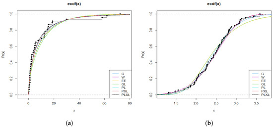
Figure 5. Fitted CDF plots for (a) data set 1, and (b) data set 2.

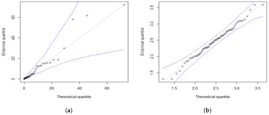
Figure 6. QQ plots with confidence bounds of the fitted PLXL model for (a) data set 1, and (b) data set 2.

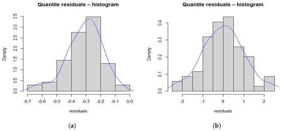
Figure 7. Histograms and PDF curves of residuals for the PLXL model for (a) data set 1, and (b) data set 2.

5.2. Modelling Censored Data

This subsection presents the analysis of a right-censored data set. The data consist of remission times (in months) from a sample of 139 bladder cancer patients [28]. Because not all patients experienced relapse before the study ended (or were lost to follow-up), some of their remission times are only known to exceed a certain duration; hence, the data are subject to right-censoring. The data set is considered below. The * in the data set indicates the censored observation.

• Data set 3 (remission times):
  4.50, 32.15, 3.88, 13.80, 19.13, 4.87, 3.02*, 5.85, 14.24, 5.71, 19.36*, 7.09, 7.87, 7.59, 20.28, 5.32, 5.49, 46.12, 2.02, 4.51, 5.17, 2.83, 9.22, 1.05, 0.20, 8.37, 3.82, 9.47, 36.66, 14.77, 26.31, 79.05, 10.06, 8.53, 4.65*, 2.02, 4.98, 11.98, 2.62, 4.26, 5.06, 1.76, 0.90, 11.25, 16.62, 4.40, 21.73, 10.34, 12.07, 34.26, 0.87*, 10.66, 6.97, 2.07, 0.51, 12.03, 0.08, 17.12, 3.36, 2.64, 1.40, 12.63, 43.01, 14.76, 2.75, 7.66, 0.81, 1.19, 7.32, 4.18, 3.36, 8.66, 1.26, 13.29, 1.46, 14.83, 6.76, 23.63, 24.80*, 5.62, 8.60*, 3.25, 10.86*, 18.10, 7.62, 7.63, 17.14, 25.74, 3.52, 2.87, 15.96, 17.36, 9.74, 3.31, 7.28, 1.35, 0.40, 2.26, 4.33*, 9.02, 5.41, 2.69, 22.69, 6.94, 2.54, 11.79, 2.46, 7.26, 2.69, 5.34, 3.48, 4.70*, 8.26, 6.93, 4.23, 3.70, 0.50, 10.75, 6.54, 3.64, 5.32, 13.11, 8.65, 3.57, 5.09, 7.39, 5.41, 11.64, 2.09, 2.23, 6.25, 7.93, 4.34, 25.82, 12.02.

The TTT plot for above data is consided in Figure 8. From the TTT plot it is clear that data has an IBT shape for HRF.

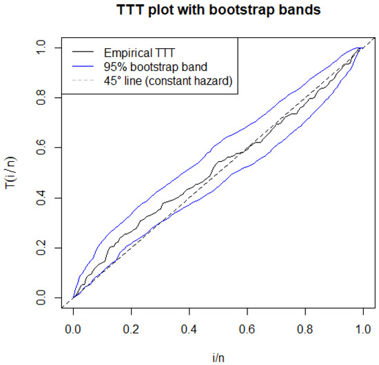
Figure 8. TTT plot of remission time data.

We fit the PLXL distribution to the remission time data and compare it to some of the standard distributions that can explain hazard rate data with an IBT shape. These distributions are as follows:

• Generalized Inverted Exponential (GIE) distribution [29]:

  $$f_{GIE}\left(x\right)={\displaystyle \frac{\lambda \theta }{x^2}}{e}^{-\theta /x}{\left(1-e^{-\theta /x}\right)}^{\lambda -1},x>0,\lambda >0,\theta >0.$$
• Inverse Gamma (IG) distribution:

  $$f_{IG}\left(x\right)={\displaystyle \frac{{\theta }^{\lambda }}{\Gamma \left(\lambda \right)}}{x}^{-(\lambda +1)}{e}^{-\theta /x},x>0,\lambda >0,\theta >0.$$
• Inverse Weibull (IW) distribution:

  $$f_{IW}\left(x\right)=\lambda \theta x^{-(\theta +1)}{e}^{-\lambda x^{-\theta }},x>0,\lambda >0,\theta >0.$$
• Inverse Power Lindley (IPL) distribution [8]:

  $$f_{IPL}\left(x\right)={\displaystyle \frac{\lambda {\theta }^2}{1+\theta }}{\displaystyle \frac{1+x^{\lambda }}{x^{2\lambda +1}}}{e}^{-\theta /x^{\lambda }},x>0,\lambda >0,\theta >0.$$
• Lognormal (LN) distribution:

  $$f_{LN}\left(x\right)={\displaystyle \frac{1}{x\theta \sqrt{2\pi }}}{e}^{-{\displaystyle \frac{{(lnx-\lambda )}^2}{2{\theta }^2}}},x>0,\lambda >0,\theta >0.$$
• Lindley-Exponential (LE) distribution [30]:

  $$f_{LE}\left(x\right)={\displaystyle \frac{{\theta }^2\lambda e^{-\lambda x}{(1-e^{-\lambda x})}^{\theta -1}\left(1-ln(1-e^{-\lambda x})\right)}{1+\theta }},x>0,\lambda >0,\theta >0.$$

In Table 6, the estimation and performance criteria values of the different models are taken into consideration. AIC and BIC are used to evaluate the performance of different models. The PLXL model performs better than other competitive models, according to AIC and BIC values. As a result, the PLXL model can be effectively used to simulate different types of lifespan data sets.

Table 6. Summary of model estimation and related criteria for the second data set.

MODEL	MLEs	AIC	BIC
GIE	$\widehat{\lambda }=0.6858$ (0.0815)	$928.8$	$931.6$
	$\widehat{\theta }=1.9620$ (0.2691)
IG	$\widehat{\lambda }=0.6650$ (0.0717)	$920.4$	$926.2$
	$\widehat{\theta }=1.7361$ (0.2613)
IW	$\widehat{\lambda }=2.2967$ (0.2091)	$896.1$	$901.9$
	$\widehat{\theta }=0.7551$ (0.0430)
IPL	$\widehat{\lambda }=0.6977$ (0.0405)	$899.5$	$905.3$
	$\widehat{\theta }=3.0817$ (0.2308)
LN	$\widehat{\lambda }=1.8290$ (0.0958)	$841.4$	$847.2$
	$\widehat{\theta }=1.0981$ (0.0692)
LE	$\widehat{\lambda }=0.1011$ (0.0129)	$834.5$	$840.3$
	$\widehat{\theta }=1.5555$ (0.1606)
PLXL	$\widehat{\lambda }=0.6712$ (0.0399)	$833.6$	$839.4$
	$\widehat{\theta }=0.5989$ (0.0596)

6. Conclusions

In this study, we introduced a novel two-parameter lifetime distribution referred to as the PLXL distribution. The corresponding model was developed to provide greater flexibility when modeling complex lifetime data, particularly in situations where traditional models struggle to capture certain hazard rate behaviors. Specifically, the PLXL distribution can model a wide range of hazard rate shapes, including increasing, decreasing, bathtub, and the most notable unimodal forms. This makes it highly suitable for modeling data from biological and reliability systems, where such hazard rate patterns are frequently observed.

We investigated the statistical properties of the PLXL distribution, including its probability density and cumulative distribution functions, moments, HRF, and other relevant reliability characteristics. We estimated the parameters using two prominent techniques: LS estimation and ML estimation. The performance of these estimation approaches was examined through an extensive Monte Carlo simulation study. The simulation results showed that the ML estimation consistently produced lower bias and MSE than the LS estimation, demonstrating superior estimation accuracy, particularly for moderate to large sample sizes.

To show the applicability and superiority of the PLXL model further, we fitted the distribution to three real-life data sets representing diverse applications. We compared the PLXL model against several well-known, widely used two-parameter lifetime models, including the gamma, Weibull, EE, GL, PL, and PXL models. Goodness-of-fit was assessed using several standard criteria, including the KS statistic and its associated p-value, AIC, and the BIC.

Across all three data sets, the PLXL model outperformed competing models. These results emphasize the robustness and adaptability of the PLXL model in accommodating a wide range of lifetime data patterns, highlighting its potential as a general-purpose model in lifetime and reliability analysis.

In conclusion, the PLXL distribution significantly extends the Lindley-type distribution family and offers enhanced capabilities for modeling lifetime data. Its theoretical tractability, combined with superior empirical performance, makes it a valuable addition to the statistician’s toolkit, particularly in fields such as biostatistics, engineering reliability, and survival analysis. Future research could explore the multivariate and regression extensions of the PLXL distribution, as well as its application to more complex censored data scenarios.

References

- Efron, B. Logistic regression, survival analysis, and the Kaplan-Meier curve. J. Am. Stat. Assoc. 1988, 83, 414–425. [Google Scholar] [CrossRef]
- Andrews, D.F.; Herzberg, A. Data: A Collection of Problems from Many Fields for the Student and Research Worker; Series in Statistics; Springer: New York, NY, USA, 1985. [Google Scholar]
- Lindley, D.V. Fiducial distributions and Bayes’ theorem. J. R. Stat. Soc. Ser. B 1958, 20, 102–107. [Google Scholar] [CrossRef]
- Ghitany, M.; Al-Mutairi, D.; Balakrishnan, N.; Al-Enezi, L. Power Lindley distribution and associated inference. Comput. Stat. Data Anal. 2013, 64, 20–33. [Google Scholar] [CrossRef]
- Ghitany, M.; Alqallaf, F.; Al-Mutairi, D.K.; Husain, H.A. A two-parameter weighted Lindley distribution and its applications to survival data. Math. Comput. Simul. 2013, 81, 1190–1201. [Google Scholar] [CrossRef]
- Nadarajah, S.; Bakouch, H.; Tahmasbi, R. A generalized Lindley distribution. Sankhya B 2011, 73, 331–359. [Google Scholar] [CrossRef]
- Sharma, V.K.; Singh, S.K.; Singh, U.; Agiwal, V. The inverse Lindley distribution: A stress-strength reliability model with application to head and neck cancer data. J. Ind. Prod. Eng. 2015, 32, 162–173. [Google Scholar] [CrossRef]
- Barco, K.; Mazucheli, J.; Janeiro, V. The inverse power Lindley distribution. Commun. Stat.-Simul. Comput. 2017, 46, 6308–6323. [Google Scholar] [CrossRef]
- Chouia, S.; Zeghdoudi, H. The XLindley distribution: Properties and application. J. Stat. Theory Appl. 2021, 20, 318–327. [Google Scholar] [CrossRef]
- Metiri, F.; Zeghdoudi, H.; Ezzebsa, A. On the characterisation of XLindley distribution by truncated moments. properties and application. Oper. Res. Decis. 2022, 32, 97–109. [Google Scholar]
- Zinhom, E.; Nassar, M.; Radwan, S.; Elmasry, A. The wrapped XLindley distribution. Environ. Ecol. Stat. 2023, 30, 669–686. [Google Scholar] [CrossRef]
- Etaga, H.O.; Nwankwo, M.P.; Oramulu, D.O.; Anabike, I.C.; Obulezi, O.J. The double XLindley distribution: Properties and applications. Sch. J. Phys. Math. Stat. 2023, 10, 192–202. [Google Scholar] [CrossRef]
- Beghriche, A.; Tashkandy, Y.A.; Bakr, M.E.; Zeghdoudi, H.; Gemeay, A.M.; Hossain, M.M.; Muse, A.H. The inverse XLindley distribution: Properties and application. IEEE Access 2023, 11, 47272–47281. [Google Scholar] [CrossRef]
- MirMostafaee, S. The exponentiated new XLindley distribution: Properties, and Applications. J. Data Sci. Model. 2023, 2, 185–208. [Google Scholar]
- Gemeay, A.M.; Ezzebsa, A.; Zeghdoudi, H.; Tanış, C.; Tashkandy, Y.A.; Bakr, M.; Kumar, A. The power new XLindley distribution: Statistical inference, fuzzy reliability, and applications. Heliyon 2024, 10, e36594. [Google Scholar] [CrossRef]
- Alghamdi, F.M.; Ahsan-ul Haq, M.; Hussain, M.N.S.; Hussam, E.; Almetwally, E.M.; Aljohani, H.M.; Mustafa, M.S.; Alshawarbeh, E.; Yusuf, M. Discrete Poisson quasi-XLindley distribution with mathematical properties, regression model, and data analysis. J. Radiat. Res. Appl. Sci. 2024, 17, 100874. [Google Scholar] [CrossRef]
- Alomair, A.M.; Ahmed, M.; Tariq, S.; Ahsan-ul Haq, M.; Talib, J. An exponentiated XLindley distribution with properties, inference and applications. Heliyon 2024, 10, e25472. [Google Scholar] [CrossRef] [PubMed]
- Musekwa, R.R.; Makubate, B. A flexible generalized XLindley distribution with application to engineering. Sci. Afr. 2024, 24, e02192. [Google Scholar] [CrossRef]
- Alsadat, N. A new extension of XLindley distribution with mathematical properties, estimation, and application on the rainfall data. Heliyon 2024, 10, e38143. [Google Scholar] [CrossRef]
- Kouadria, M.; Zeghdoudi, H. The truncated new-XLindley distribution with applications. J. Comput. Anal. Appl. 2025, 34, 53–64. [Google Scholar]
- Wang, X. A simple proof of descartes’s rule of signs. Am. Math. Mon. 2004, 111, 525–526. [Google Scholar] [CrossRef]
- R Core Team. R: A Language and Environment for Statistical Computing; R Foundation for Statistical Computing: Vienna, Austria. 2025. Available online: https://www.R-project.org/ (accessed on 26 August 2025).
- Swain, J.; Venkatraman, S.; Wilson, J. Least squares estimation of distribution function in Johnson’s translation system. J. Stat. Comput. Simul. 2025, 29, 271–297. [Google Scholar] [CrossRef]
- Johnson, N.; Kotz, S.; Balakrishnan, N. Continuous Univariate Distribution; John Wiley: New York, NY, USA, 1995. [Google Scholar]
- Almongy, H.M.; Almetwally, E.; Ahmad, H.; Al-nefaie, A. Modelling of COVID-19 vaccination rate using odd Lomax inverted nadarajah-haghighi distribution. PLoS ONE 2022, 17, e0276181. [Google Scholar] [CrossRef]
- Aarset, M. How to identify a bathtub hazard rate. IEEE Trans. Reliab. 1987, 36, 106–108. [Google Scholar] [CrossRef]
- Gupta, R.; Kundu, D. Exponentiated exponential family: An alternative to gamma and Weibull distributions. Biom. J. 2001, 43, 117–130. [Google Scholar] [CrossRef]
- Lee, E.; Wang, J. Statistical Methods for Survival Data Analysis; John Wiley and Sons: New York, NY, USA, 2003. [Google Scholar]
- Abouammoh, A.; Alshingiti, A. Reliability estimation of generalized inverted exponential distribution. J. Stat. Comput. Simul. 2009, 79, 1301–1315. [Google Scholar] [CrossRef]
- Bhati, D.; Malik, M.; Vaman, H. Lindley–exponential distribution: Properties and applications. Metron 2015, 73, 335–357. [Google Scholar] [CrossRef]
Disclaimer/Publisher’s Note: The statements, opinions and data contained in all publications are solely those of the individual author(s) and contributor(s) and not of MDPI and/or the editor(s). MDPI and/or the editor(s) disclaim responsibility for any injury to people or property resulting from any ideas, methods, instructions or products referred to in the content. |
© 2025 by the authors. Licensee MDPI, Basel, Switzerland. This article is an open access article distributed under the terms and conditions of the Creative Commons Attribution (CC BY) license.