Article

Semi-Supervised Machine Learning Method for Predicting Observed Individual Risk Preference Using Gallup Data

by
Faroque Ahmed
1,2,
Mrittika Shamsuddin
3,
Tanzila Sultana
4 and
Rittika Shamsuddin
5,*
1
Graduate School of Economics and Management, Ural Federal University, Lenin Ave., 51, Yekaterinburg 620075, Russia
2
Bangladesh Institute of Governance and Management, E-33, Sher-E-Bangla Nagar, Dhaka 1207, Bangladesh
3
Department of Economics, Dalhousie University, 6299 South St., Halifax, NS B3H 4R2, Canada
4
Department of Economics, College of Business Administration, Southern Illinois University, Carbondale, IL 62901, USA
5
Department of Computer Science, Oklahoma State University, Stillwater, OK 74078, USA
*
Author to whom correspondence should be addressed.
Math. Comput. Appl. 2024, 29(2), 21; https://doi.org/10.3390/mca29020021
Submission received: 28 December 2023 / Revised: 23 February 2024 / Accepted: 8 March 2024 / Published: 15 March 2024
(This article belongs to the Section Social Sciences)

Abstract

:
Risk and uncertainty play a vital role in almost every significant economic decision, and an individual’s propensity to make riskier decisions also depends on various circumstances. This article aims to investigate the effects of social and economic covariates on an individual’s willingness to take general risks and extends the scope of existing works by using quantitative measures of risk-taking from the GPS and Gallup datasets (in addition to the qualitative measures used in the literature). Based on the available observed risk-taking data for one year, this article proposes a semi-supervised machine learning-based approach that can efficiently predict the observed risk index for those countries/individuals for years when the observed risk-taking index was not collected. We find that linear models are insufficient to capture certain patterns among risk-taking factors, and non-linear models, such as random forest regression, can obtain better root mean squared values than those reported in past literature. In addition to finding factors that agree with past studies, we also find that subjective well-being influences risk-taking behavior.

1. Introduction

Individuals, as influential social and economic agents, shape economic and market dynamics through their decisions. Consequently, gaining insights into the factors influencing these decisions is crucial for predicting market changes. A pivotal factor complicating market predictions is individuals’ varying risk preferences, particularly evident during uncertain scenarios such as the housing bubble crisis [1].
The intertwined relationship between risk, uncertainty, and economic decisions is well-established [2]. However, the degree of willingness to take risks varies among individuals, influenced by both dynamic factors such as context (social, interpersonal, etc.) and temporally static factors such as Intelligence Quotient (IQ) [3,4].
Presently, two methods are employed to collect data on individuals’ risk preferences: stated risk-taking preferences and observed risk-taking preferences (ORP). ORP, favored for providing objective insights, analyzes behavioral displays across various economic activities such as stock market transactions, gambling, insurance policy purchases, medical risk, etc. The Global Preference Survey (GPS) 2012 dataset, for instance, obtains ORP through quantitative and qualitative questions [5].
While existing research mainly focuses on qualitative questions and specific countries, the GPS dataset offers a unique opportunity to explore cultural and subjective well-being influences on risk preferences across countries. This paper pioneers the investigation of common determinants of risk-taking preferences across multiple countries, utilizing GPS data from a subset of Gallup World Poll respondents for the year 2012.
The research introduces a novel approach using machine learning to predict ORP values for the entire Gallup dataset, extending beyond 2012. Traditional methods, often limited to linear regression, fail to capture the potential non-linear patterns in socioeconomic variables influencing risk tolerance. By incorporating machine learning, this study aims to unveil these non-linear patterns and identify previously overlooked independent variables relevant to individual risk tolerance.
An overview of our approach is provided in Figure 1 and Figure 2. Figure 1 is the overview of the predictive regression scheme, which shows that labeled data (e.g., merged data of D1 and D2) is used in the base learner for training. Then unlabeled data (D3) is integrated into the model using the semi-supervised model to pair unlabeled data with predicted ORP. Figure 2 shows the implementation of the regression module on datasets grouped by different sets of independent variables: (i) a dataset of potential covariates by surveying past literature or based on economic theory (and hence is considered to be the domain expert feature set) and is denoted by D E x p e r t , (ii) a dataset consisting of all usable features with no or few missing values from the original dataset, denoted by D P o s s i b l e , and finally (iii) a third, where the features were chosen by the computational model (e.g., the computational expert) and are denoted by D C o m E x . As shown in Figure 2, D P o s s i b l e leads to D C o m E x .
Our findings show that the independent variables are indeed non-linearly related to ORP and that subjective well-being variables such as health status, optimistic index, corruption, and social network should be considered for studying individual risk tolerance. This underscores the need for further investigation into these variables within social and causal settings.
Our contributions can be summarized as follows:
  • Using semi-supervised learning, we expanded the prediction of ORP (collected in 2012) to the Gallup dataset, covering the years 2006–2018.
    We further propose an evaluation step, in addition to traditional evaluation techniques, to ensure the validity of the expansion.
  • By integrating a non-linear regression model with the commonly used Ordinary Least Squares (OLS) model, our research opens avenues for uncovering non-linear patterns in predicting general willingness to take risks.
  • Our study identifies four factors—health status, optimistic index, social network, and corruption—that were previously overlooked but emerge as potentially significant contributors to determining individual risk tolerance.
The rest of the paper is organized as follows: Section 2 shows the literature review, Section 3 provides detailed methodology with different subsections for semi-supervised methods, Section 4 presents analytical results, and Section 5 provides the conclusion.

2. Literature Review

The concept of risk-taking preferences is investigated from many different perspectives, including financial, personal decision-making, psychological, and social activities, and many others. Several research studies have investigated the factors that may explain the willingness to take general and financial risks. These studies mostly used large individual datasets of individual risk preferences and their sociodemographic, economic behavior, and self-reported data on risk preference.
Using German socioeconomic panel (SOEP) data, ref. [6] incorporated panel fixed effect regression and the ordered logit model. They found that an individual’s willingness to take risks changes when changes in family structure (separation of parents, birth of child, marriage, etc.) occur. They analyzed that positive changes in family structure (i.e., birth, marriage) decrease the individuals’ risk tolerance. In contrast, negative changes (i.e., separation of parents, providing long-term care) result in a rise in risk tolerance. Ref. [7] found that intergenerational transmission of willingness to take risks, in general, is strong between parent and child when that child has fewer siblings and is first born, using SOEP data and OLS regression. They also state that the gender of the child does not matter in the case of intergenerational transmission of risk preference. Ref. [8] found that socialization is important in the process of intergenerational risk transmission, using the same dataset and data analysis model. Ref. [2] used SOEP data together with data from a field experiment on 450 subjects and found that gender, age, height, and parental background have a significant economic impact on the respondent’s willingness to take a general risk using interval regression techniques. Ref. [1] showed that respondents’ outlook on favorable or unfavorable outcomes of risky situations affects their general willingness to take a risk, and the idea of risk is strongly linked with the individual’s optimism and a stable facet of personality. Here, they used the data from 348 participants and OLS regression.
Ref. [9] computed the Coefficient of Relative Risk Aversion (CRRA), utilizing parameters collected from 6000 observations taken from data pertaining to the US stock market. This estimation involved using a simulation technique with 100 replications. Focusing on insurance demand or consumption, ref. [10] conducted a review of empirical works of literature in order to gain a better understanding of Relative Risk Aversion (RRA) in two primary areas: first, the measurement and magnitude of risk aversion and second, the sociodemographic variables that are associated with risk aversion.
According to [11], the stated general risk preference or willingness to take general risk is collected by asking the respondents how willing they are to take a risk. They indicated that emotional expressions act as cues to the individual’s willingness to take risks in five different risk domains. These risk domains are as follows: ethical, financial, health and safety, recreational, and social. Researchers have worked on understanding what factors influence these risk-taking attitudes and found that various social, psychological, and economic factors play a significant role in determining risk-taking behavior. This research focuses mostly on the social, psychological, and economic aspects of general risk-taking assessment. Ref. [5] found that female individuals are more risk-averse than male individuals in the case of both financial and general risk-taking. They also showed that there exists a negative correlation between age and the willingness to take general risks and that the risk-taking concept is strongly associated with patience, using the global preference survey (GPS) data and OLS regression analysis. Ref. [12] showed that general risk preference exhibits large variation across and within the country using GPS data. They analyzed that this variation is due to both individual-specific characteristics (gender, age, cognitive skills, patience, trust, etc.) and collective characteristics (cultural and biogeographical aspects) using regression analysis with OLS estimators. In the case of financial risk tolerance, the study of [13] suggests that respondent’s characteristics (gender, age, marital status), personality (economic expectation), and socioeconomic background (occupational status, income, education, financial knowledge) can be used as a determinant of individual’s risk preference. Using a sample of 1075 university faculty and staff, descriptive discriminant analysis, univariate test statistics, and F test for data analysis, they found that male, older, married, and professional respondents with a higher level of income, education, financial knowledge, and economic expectation were more risk-tolerant. Ref. [14] found that, although race and ethnicity affect financial risk preference, it is conditional upon other variables, such as financial education. They used a survey of consumer finances (SCF) datasets, incorporated a cumulative logit model for data analysis, and concluded that financial risk preference varies among different groups. Ref. [15] investigated the relationship between self-reported data on the financial risk-taking willingness and social and state “cushioning” using Luxembourg wealth study database. This database consists of large-scale household data for three countries with different social-safety support networks. They showed that individual willingness to take financial risks is highly influenced by state cushioning, using stepwise multiple linear regression.
These studies on general and financial risk preference mostly kept their investigation limited to analyzing the association and correlation between the sociodemographic and economic data and using the self-reported (general or financial) willingness to take the risk. To the authors’ best knowledge, no study has used the techniques of semi-supervision machine learning to predict either individuals stated or observed willingness to take general risks. This study combined both linear regression and other techniques of machine learning (semi-supervised method) to explore the relationship between social and economic covariates of ORP. Another contribution of this article over related studies, which uses similar data, is that based on available risk-taking data, we are proposing an approach that can efficiently predict ORP for those countries/individuals with missing ORP. Moreover, unlike previous investigations, we attempt to find features that better explain ORP based on an algorithm.

3. Methodology

3.1. Overview of the Proposed Methodology

This study’s variable of interest or target variable is the observed willingness to take general risks or the Observed Risk-taking Preference (ORP) from the Global Preference Survey (GPS) dataset. The Appendix A explains how the risk preference index is calculated in the GPS data. Due to the advantages of studying risk preference using an objective, continuous target variable (such as ORP), in this paper we focus on (i) predicting ORP to the Gallup dataset, (ii) investigating non-linear patterns, and (iii) finding/identifying more predictors of ORP. As such, these objectives guide this paper’s methodology, experimentation and designs.
Step 1: Merging the GPS and Gallup Datasets: The Global Preference Survey (GPS) dataset has data from 79 countries for the year 2012, along with the variable of interest (e.g., ORP), whereas the Gallup dataset contains data of the same 79 countries over a period covering from 2006 and 2018. Since the GPS data collection was an extension of the general Gallup data collection, both datasets share a set of shared independent variables. Thus, the two datasets were merged using the Gallup id as the primary key. The resulting dataset has 2671 independent variables with ORP values for 2012 only, and missing ORP values for 2006–2011 and 2013–2018. In computation, predicting missing target variable values falls under semi-supervised machine learning (ML), leading to the development of the predictive regression scheme (Figure 1) described in Step 2.
Step 2: Semi-Supervised Learning: An algorithm that learns from both labeled and unlabeled data is known as semi-supervised learning [16]. In this case, any data point with a known ORP value is considered labeled data, while any data point with a missing ORP value is referred to as unlabeled. Generally, the semi-supervised predictive models learn to predict ORP values for unlabeled data points using information gained from a set of labeled data points. This usually consists of initial training an ML-supervised model, called a base learner, on the labeled data points. The unlabeled data points are then incorporated into the model iteratively, as described in Section 3.4.2. To incorporate the scholarly knowledge from previous studies on risk preference, we use linear regression models (trained via the OLS method) as our base learner for finding linear patterns, while non-linear models such as Random Forest and SVM regression models are used as the base learner to explore non-linear patterns. Next, to incorporate the unlabeled data, we choose self-training to predict ORP for the Gallup dataset.
Step 3: Evaluation Scheme for the Predictive Regression Models: To the best of our knowledge, a semi-supervised learning paradigm has yet to be applied for predicting risks in a socioeconomic context. That is why it is important in this paper to provide a comprehensive evaluation framework of the base leaner and models from each iteration to ensure the validity of the proposed approach. As such, each model is evaluated first via established traditional ML evaluation schemes and traditional regression evaluation schemes (Figure 3). In addition, to ensure that the predicted ORP values for unlabeled data points are following the assumptions of the semi-supervised paradigm, we propose (i) the use of plots for visual evaluation and (ii) the use of comparative evaluation. An overview of the evaluation can be found in Figure 3. More details are provided in Section 3.5.
Step 4: Feature Exploration: In order to identify features that are generally not studied in association with individual risk but might still have a significant influence on ORP, Steps 2 and 3 are repeated three times on the merged dataset from Step 1. On the first repetition, the independent variables are based on commonly used covariates in the literature; we refer to this dataset as D E x p e r t . During the second, all variables from the merged dataset that could be included (e.g., variables with less than 50% missing values) were used to train the models; this dataset is referred to as D P o s s i b l e . Finally, the models were trained on a feature set, resulting in a dataset referred to as D C o m E x , that was shown to be significant in predicting ORP based on results from the previous repetition, e.g., D C o m E x is a proper subset of the features in D P o s s i b l e .

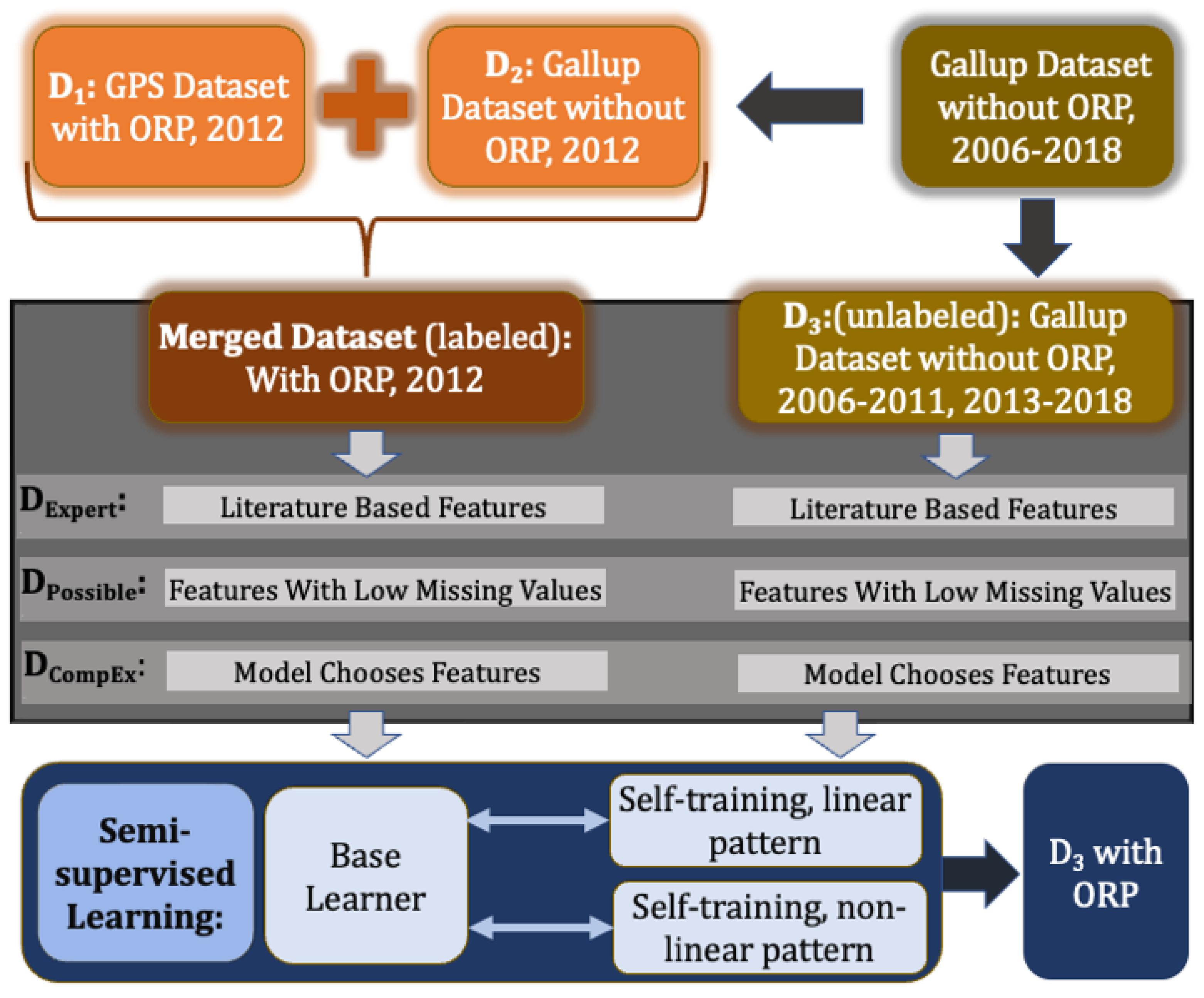
3.2. Dataset Description: GPS, Gallup, Merged

Gallup’s World Poll uses random, nationally representative samples to question citizens in more than 150 countries, representing more than 99% of the world’s adult population. Gallup surveys 1000 people in each nation using a standard set of core questions that have been translated into the respective country’s primary languages. Supplementary questions are asked in some places in addition to core questions. Face-to-face interviews last around an hour, while phone interviews last about 30 min. The survey is done once a year in many countries, and fieldwork is typically finished in two to four weeks. Gallup is solely responsible for the administration, design, and implementation of the Gallup World Poll. The Gallup World Poll covers important indices relating to global development, including law and justice, housing, creating jobs, migration, financial life, health status, civic involvement, and overall well-being. These indicators help economic and policy leaders grasp the country’s interests’ wider context while establishing particular links between indexes and trailing economic results. Gallup gathers samples in metropolitan areas or areas of special interest in various nations. In some major nations, such as China and Russia, a representative sample of at least 2000 persons is anticipated.
Global Preference Survey (GPS) data is an extension of Gallup questions for the year 2012, where they play games to observe the risk-taking index ORP, which is the target variable of this study. There are 15 columns, which are the additional questions to the Gallup World survey that were asked to the 80,337 (rows) respondents in the dataset.
Merged Dataset: Both Gallup and GPS data have been merged for 2012 by Gallup id to get the final dataset for 2012, including the target variable ORP. The merged data consists of 79 countries with 80,337 observations and 2672 columns.
Gallup Dataset without ORP: This is the part of the Gallup’s World Poll that does not have the ORP label and hence, did not end up in the Merged Dataset. It contains data from 2006 to 2011 and 2013 to 2018, and has over a million data points. However, since we had to filter the dataset to include data points that have the features obtained from literature and data points with low missing value count, we end up with 634 observations from this dataset.

3.3. Data Preprocessing

Data Transformation: There are both categorical and numerical variables in the dataset. Most of the categorical variables have two categories. That is why standardization of other numerical variables is required to have a unique scale. Different methods of standardization have been applied to the numerical variables, i.e., (0, 1) scaling, Z-score scaling, dividing each value by the range, dividing each value by the standard deviation, (1, 2) scaling, etc. Finally, (1, 2) scaling is chosen.
Additionally, data transformation is a crucial data pre-processing method that can aid with inferential estimations. It transforms the data into clean, usable data by altering its format, structure, or values. In this article, we experiment with different combinations of variable transformations: four different transformations for the dependent variable (i.e., 1 y , 1 e y , 1 y 2 , and 1 y ) and two different transformations of the independent variables [ ln ( x ) , x 2 ] . The transformed variable combination that maintained the general assumptions of OLS linear regression was kept to train the base learners in this paper. Potential outliers were identified and accordingly trimmed using the said combination of the variable transformations. As an example, all the variables from D E x p e r t and their respective transformations are shown in Table 1, where the chosen transformations for each variable are bold-faced.

3.4. Semi-Supervised Learning Using Self-Training Method

As mentioned earlier, semi-supervised learning is a well-established computational learning paradigm that aids in predicting missing target variables (as opposed to independent variables). Similar to linear regression, the semi-supervised paradigm operates on some basic assumptions [17]:
  • The smoothness assumption: if two instances x and x are close together in the input space, their labels y and y should display similar proximity
  • The low-density assumption: the discriminator/classifier should not pass through high-density regions in the input space
  • The manifold assumption: data points on the same low-dimensional manifold should have the same label or similar values.
Most semi-supervised learning techniques are built on these assumptions, and they often rely on a single or all of them being fulfilled, either explicitly or implicitly. Self-training procedures (also known as “self-learning” methods) are the most fundamental of pseudo-labeling procedures under a semi-supervised learning paradigm. Under the self-training paradigm, a single supervised classifier (called the base learner) is repeatedly taught on both labeled and pseudo-labeled data from earlier rounds of the method. As a starting point, a supervised classifier is trained on just the labeled data at the start of the self-training phase. This classifier is then utilized to make predictions for the unlabeled data points. The most confident forecasts are then introduced to the labeled training set, and the supervised classifier is re-trained using both the original labeled data and the newly generated pseudo-labeled data. This method is usually repeated until no unlabeled data remains.

3.4.1. Base Learners

In general, when there is an ensemble of predictive learners (e.g., independent learners) or learners are changed over time (one learner is dependent on the next through time), the term base learner is used to refer to either the individual independent learners or to the learner that drives the entire cast of dependent learners. Here, we use only one supervised machine learning model as the base learner, which is first trained on the few labeled data, and then re-trained on the addition of pseudo-labels. Since OLS linear regression is widely used in social studies, we use OLS linear regression model as the base learner for exploring linear patterns. For non-linear patterns, we use non-linear regression models.
Linear Regression, LR: Linear regression is a fundamental and widely used type of predictive model. The overall goal of regression analysis is to answer the following questions: (i) how well does a collection of predictive features (e.g., independent variables) predict an outcome variable (e.g., target variable)? and (ii) which factors, in particular, are significant predictors of the outcome variable, and how do they influence it (as indicated by the size and sign of the beta estimates)? Diagnostic tests like RMSE, Breusch-Pagan test, and Ramsay RESET test can be used to see if the model fitted well or not. The general equation of multiple linear regression is Y = β 0 x 0 + β 1 x 1 + + β n x n + ε . Y is the target variable which depends on the values of some regressors x 1 , x 2 , , x n with coefficients denoted by β i , respectively. Note, x 0 = 1 and hence β 0 is the intercept term of the model.
Random Forest Regression, RFR: Similar to Random Forest Classifiers [18], RFR [19,20] utilizes a collection of Decision Trees [21] to arrive at a prediction. Each tree in the “forest” makes a prediction which is then aggregated using techniques of ensemble machine learning models [22]. Each tree learns a non-linear separation of the feature space by optimizing feature threshold values for relevant or significant features. Since each decision tree learns a non-linear boundary, the RFR also learns a non-linear boundary. Assume, that each decision tree is denoted by the function h i ( x , θ k ) , where h i : x R and θ k is the set of parameters for the model, then an RFR can be defined as: Y = ( 1 / N ) i = 1 N h i ( x , θ k ) , where N is the total number of decision trees in the collection.
Support Vector Regression, SVR: The non-linear dual formulation of SVR makes use of LaGrange multipliers and non-linear kernel functions (which can also be represented by semi-definitive Gram matrices) to find an optimal non-linear hypersurface to separate the data in feature space. A detailed description of SVR dual formula derivation is outside the scope of this paper but can be found in [23]. SVR prediction written as a function can be expressed as: Y = n = 0 N ( α n α n * ) K ( x n , x ) , where n is the number of instances, x are the feature vectors, K is the kernel matrix/function, α n are the Lagrange multipliers.
Gradient Boost Regression, GBR: GBR [24] is a non-linear, additive ensemble of Decision Trees. However, unlike RFR, each individual model in the GBR is trained specifically to learn to predict on data instances that were incorrectly predicted by the previous model/learners and is, thus, described recursively. Then during the mth iteration of GBR: Y m = Y m 1 + ρ m h m ( x , θ k ) , where Y m 1 is the accumulated prediction from the previous learners, h m is the newly added decision tree, and ρ m , is the associated weight for the learner.

3.4.2. Self-Training—Iterative Training of a Base Learner

Figure 4 illustrates the recursive training and re-training of base learners in the self-training paradigm of semi-supervised learning. Before the training begins, D3-the Gallup data without ORP labels, is split into ten partitions or batches, such that each batch consists of 10% of non-overlapping instances/observations from D3. This is done in preparation for the Proposed Iterative Evaluation Scheme, which will be detailed in Section 3.5.2. More specifically, D3 contains a total of 634 observations, resulting in 9 partitions of 63 observations and one partition of 67 observations.
During the first iteration of this training process:
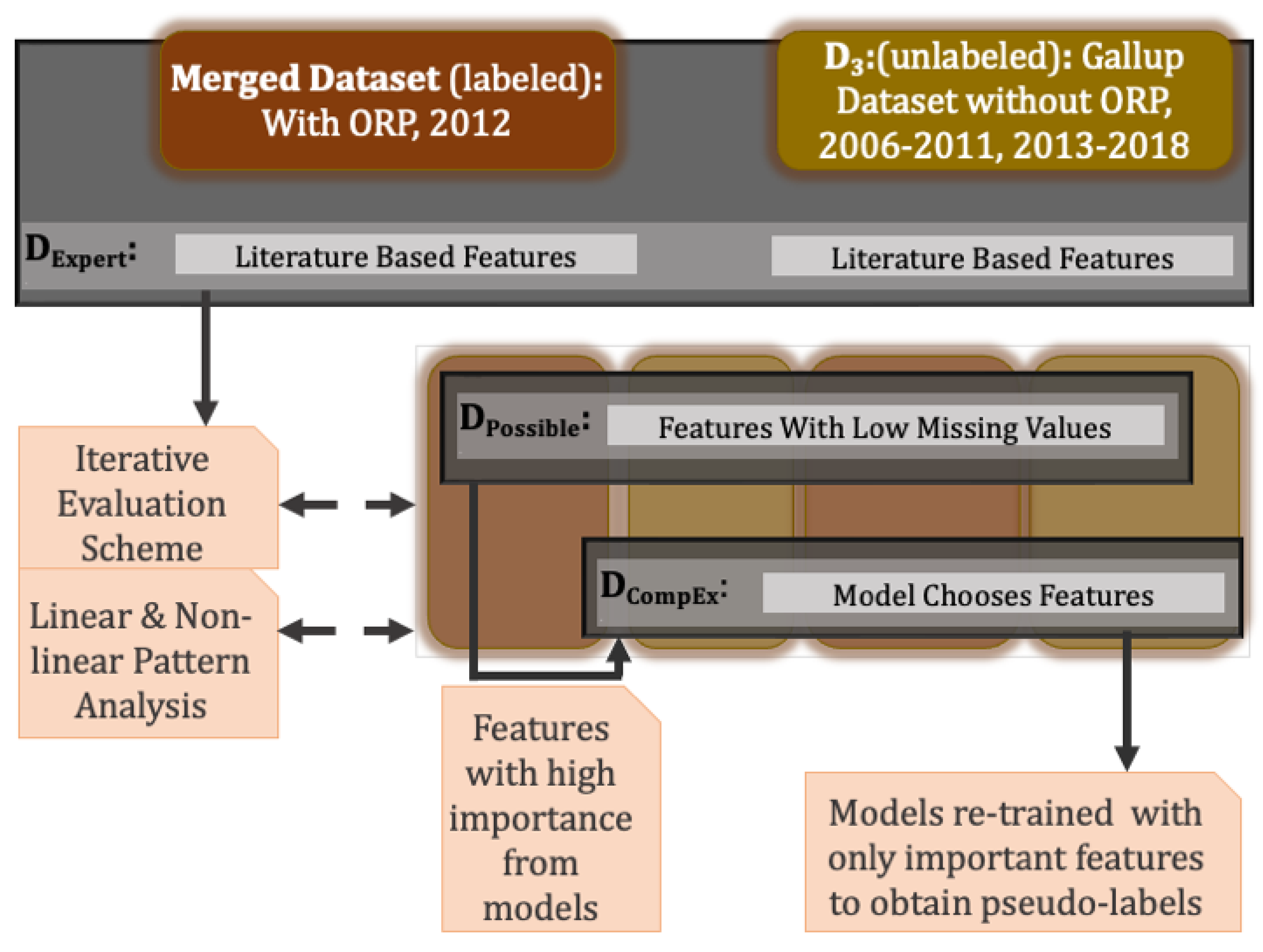
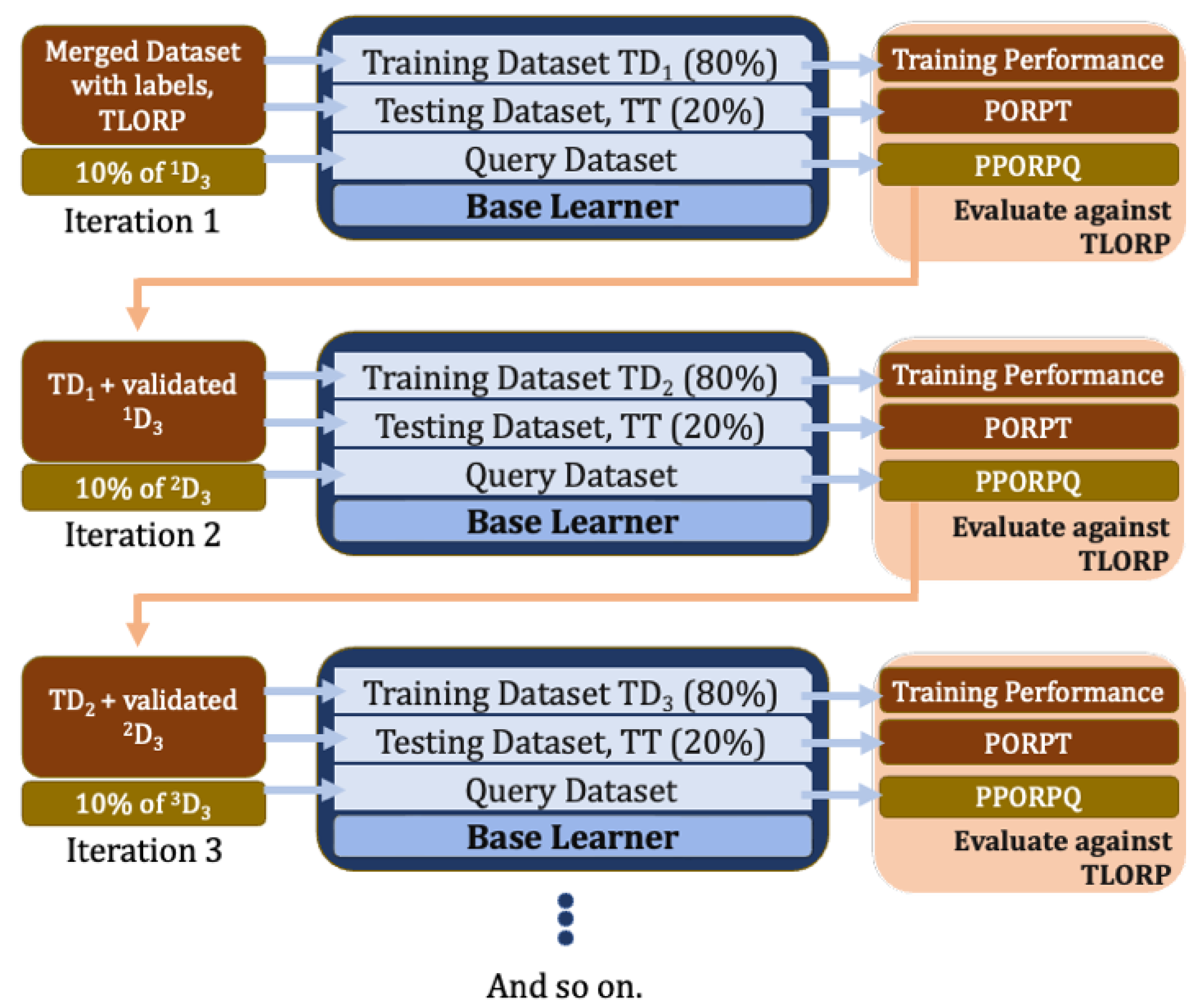
  • Step 1: The base learner is trained using the merged training dataset (Figure 4) from D1 and D2, e.g., the one where Gallup data are directly associated with the ORP values from GPS 2012 dataset. Since the 2012 dataset contains authentic ORP values, these values are referred to as True Label ORP (TLORP).
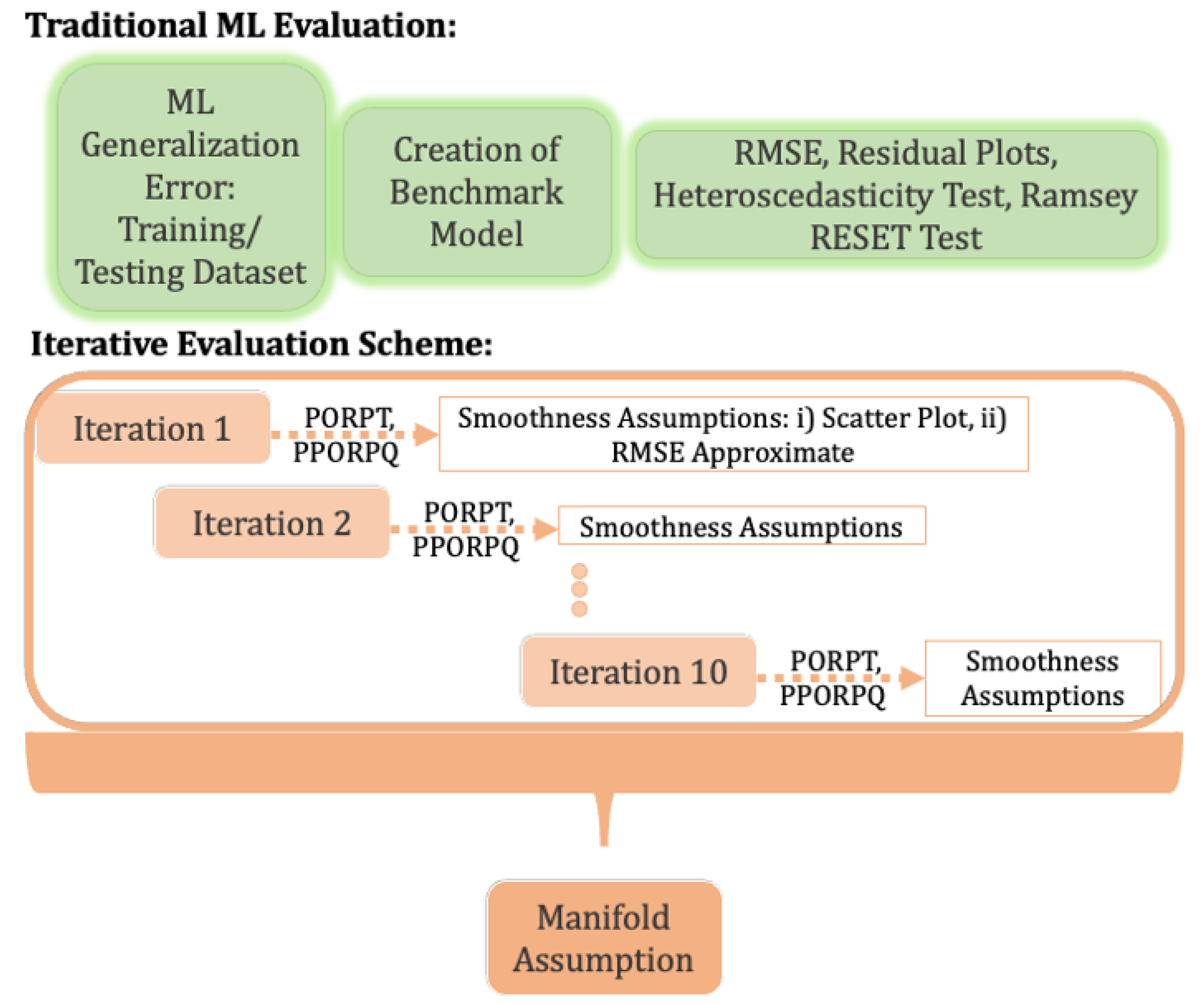
    Using traditional ML evaluation techniques for regression models, we evaluate the base learner on the test dataset (Section 3.5.1) to obtain predicted ORP (PORPT). This involves comparing the TLORP with the PORPT values. These predicted results are recorded for later use in the process.
  • Step 2: Next, one of the ten batches from D3 is used as a query to obtain their respective prediction, e.g., the pseudo-ORP values (e.g., PPORPQ) from the base learner.
    Traditional ML evaluation metrics (such as RMSE, etc.) cannot be used to evaluate these predictions, since the query set does not have TLORP against which to calculate the RMSE value. Instead, we use the Proposed Iterative Evaluation Scheme (detailed in Section 3.5.2), a series of tests allowing us to weed out outliers within the query set.
  • Step 3: Before going on to the next iteration, the new training set is prepared. The new training set consists of: (i) the training set used in Step 1 of this iteration and (ii) observations in the query set from Step 2 that passed the Proposed Iterative Evaluation Scheme. The testing set remains untouched and is kept constant during each iteration.
These steps are repeated until data from all ten batches have been incorporated in the training set of the base learner and have been used to predict the test dataset, which does have TLOPR associated with it. This also forms the basis of the Proposed Iterative Evaluation Scheme.

3.5. Evaluation Scheme

This section describes the scheme used in this paper to evaluate the semi-supervised models trained via self-training. Since most ML studies for risk use supervised learning, we use the performance of a similar supervised ML model as the benchmark and include descriptions for evaluating the benchmark.

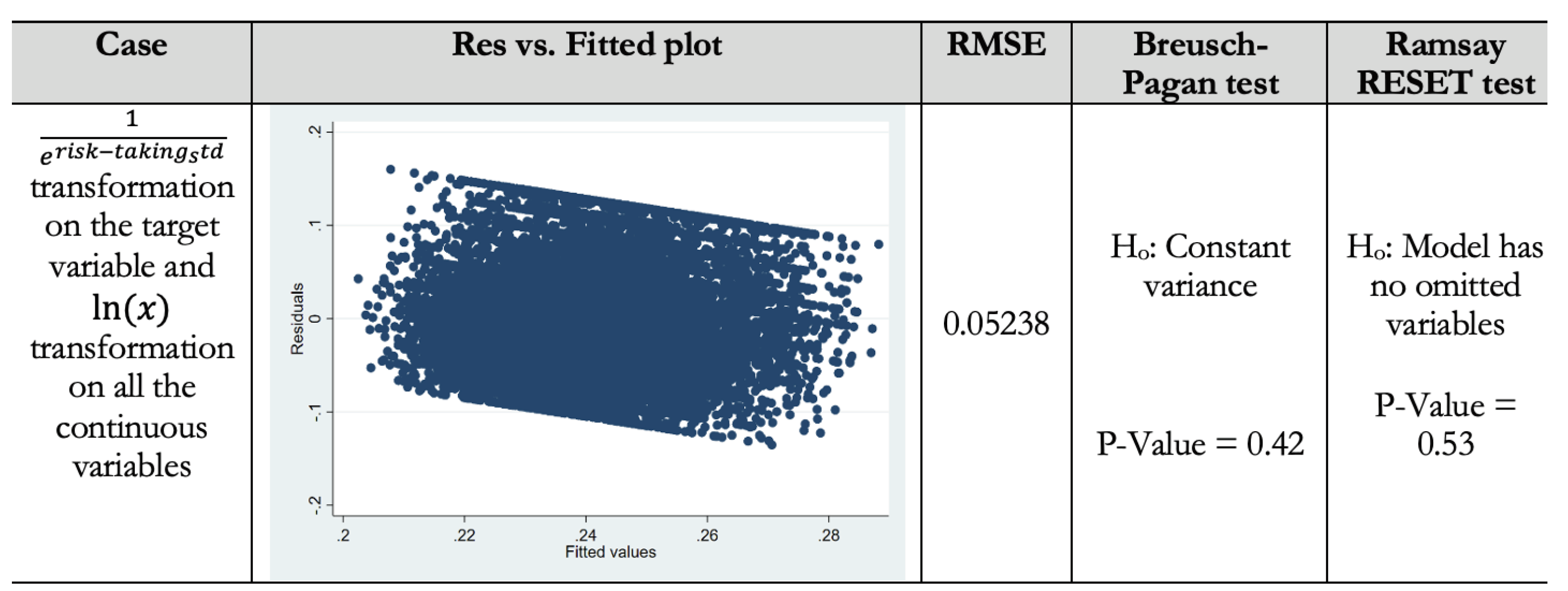
3.5.1. Traditional ML Evaluation

The purpose of training ML models is to teach a machine about a concept in the real world. And similar to the real world, where a child is expected to apply things they learn to their life as it is happening, it is expected that a trained ML model will be able to make predictions based on data it has not seen during training. The child/model has properly learned the material only if they are able to use the learned information when presented with a previously unseen situation. Thus, to evaluate the suitability of a supervised ML model for classification or prediction, it is imperative to divide the dataset into two, creating the training and testing datasets. The model uses the training dataset to learn, while the testing dataset is the exam paper they must pass to be considered suitable. The error on the test dataset is a measure of the generalization error; the higher the error, the lower the ability of the model to generalize and apply what it has learned, if at all. The higher the accuracy of the model, the lower its generalization error. It is usual for the training-testing split ratio to be 80:20 or 70:30. In this paper an 80:20 split is used to obtain and evaluate the PORPT (Section 3.4.2, Step 1).
Establishing a Benchmark: As with all other scientific studies, to evaluate the suitability of a proposed ML model for an application, the model is compared to a similar, established model called a benchmark. This benchmark represents a model state before applying the proposed changes. Thus, compared to the benchmark, if the experimental model with the proposed changes obtains a better accuracy, then the proposed changes are considered valuable. In this paper, the experimental models are semi-supervised models trained via self-training. Thus, the benchmark used in this paper is the linear regression (LR) model which was trained and tested using the merged Gallup and GPS for the Year 2012 only. Since the Year 2012 has the TLORP (true labels) from the dataset itself, the model can be evaluated using standard supervised ML techniques and hence work as a benchmark model. Another reason to use it as a benchmark model is that this model represents the model created in Step 1 of the supervised self-training process for the LR model. The LR model is given priority as the benchmark because most studies in the literature use OLS LR models for studying risk. As such, the independent variables for this model are chosen according to past literature.
Traditional Metric Used for Evaluation of the Benchmark Model: To verify whether the model is trained properly and whether the model generalizes well, appropriate evaluation metric needs to be used on the model output (e.g., compare PORPT against TLORP). For the benchmark LR model, the regression assumptions can be used for evaluating the models. For checking the goodness of fit of the base learner RMSE, the Breusch-Pagan (BP) test for heteroscedasticity and the Ramsey RESET test of model specification will be examined.
RMSE: RMSE is defined as the square root of the mean square of all errors. R M S E = 1 n i = 1 n Y i O i 2 where O i are the observations, Y i is the predicted values of original observations, and n is the number of observations available for the analysis.
Fitted vs. Residual Plot: In order to visualize the prediction error vs. fitted values, a residual vs. fitted plot is essential.
Heteroscedasticity Test: The assumption that the residuals are distributed with homogeneity of variance at each level of the predictor variable is one of the fundamental tenets of linear regression. Homoscedasticity is the name for this presumption. We claim that heteroscedasticity is evident in the residuals when this presumption is broken. The Breusch-Pagan test is a formal statistical test that may be used to detect whether heteroscedasticity is present. The following alternative and null hypotheses are used in this test:
Null hypothesis—There is homoscedasticity (the residuals are distributed with equal variance).
Alternative hypothesis—There is heteroscedasticity (the residuals are not distributed with equal variance).
We reject the null hypothesis and accept that there is heteroscedasticity in the regression model if the p-value of the test is less than a certain threshold of significance (i.e., =0.05).
Ramsey RESET Test: A generic specification test for the linear regression model is the Ramsey Regression Equation Specification Error Test (RESET) test. The null hypothesis states that the model has no omitted variables since there is no link between the powers of the fitted values and the dependent variable. The alternative to this statement is that the model has an issue with missing variables. So, we reject the null hypothesis and conclude that the model has an issue with missing variables if the p-value of the test is less than a certain threshold of significance (i.e., = 0.05 ).

3.5.2. Proposed Iterative Evaluation Scheme

Using traditional ML evaluation techniques, such as RMSE, involves comparing the true labels (in this case, the TLORP) with the predicted labels (in this case, the PORPT). However, for models trained via a semi-supervised training paradigm, the predicted pseudo-label for the query (PPORPQ) cannot be compared to the true labels because they do not exist. Thus, to evaluate the experimental models trained via self-training, we leverage two of the three assumptions (see Section 3.4) of semi-supervised learning: the manifold assumption and the smoothness assumption. Suppose both these assumptions hold for each of the models obtained during a particular iteration of self-training. In that case, we can be confident in the pseudo labels provided by the model. The set of observations that violate these assumptions during any iteration lowers our confidence in the pseudo labels provided for the observation and hence are excluded from the training set for the next iteration. Since three tests are conducted (two for smoothness assumption and one for manifold assumption described below), the rule for exclusion is as follows:
  • If the observation passes at least one of the smoothness assumption tests, then it is not excluded; otherwise, they are excluded.
  • Next, after the completion of all iterations, if the model passes the manifold assumption, no action is taken; otherwise, we step back and re-run the smoothness assumptions with stricter conditions that if observations do not pass both smoothness assumption tests, they are excluded.
  • If the manifold assumption still fails, we conclude that the semi-supervised model should not be trusted, and a different model should be considered.
Checking the Manifold Assumption: One way to test the manifold assumption is to perturb the data slightly and observe how it affects model predictions. If small perturbations result in significant changes in predictions, it might indicate that the data is not lying on a smooth manifold e.g., a small change changes the separation manifold (or class boundary) learned by the model. We achieve this during self-training by devising the Iterative Error Test described below. The gist of the test is as follows: when two models trained on slightly different training datasets (denoted by T D 1 and T D 2 ) but tested on the same testing dataset (denoted by T T ), make similar predictions, we can deduce loose equivalency for the two training datasets from the two models (denoted by M 1 and M 2 ). Since violation of assumption would increase error and reduce accuracy, we can extrapolate the equivalence of the manifolds learned by the two models.
Iterative Error Test: Let’s revisit the self-training process. We begin with one model (e.g., M 1 ) trained on one training dataset (e.g., T D 1 ) and tested on one testing dataset (e.g., T T ); this is Step 1 described in Section 3.4.2. In Step 3 of the same iteration, we obtain a second slightly larger training dataset (e.g., T D 2 , where T D 2 = T D 1 + f i r s t q u e r y s e t p s e u d o l a b e l s ). In the next iteration, a new model (e.g., M 2 ) is trained on T D 2 and tested on T T . Thus, if the error of M 2 (on T T ) does not increase compared to M 1 , then T D 1 is equivalent to T D 2 , e.g., the query set and the pseudo labels do not violate any assumptions or data distribution.
Checking the Smoothness Assumption: Directly studying the smoothness and low-density assumption would require knowledge of the joint distribution of the variables, which is computationally expensive and intractable. Thus, we use the smoothness assumption to make an approximation. The smoothness assumption, mentioned in Section 3.4, can be interpreted to say that for any two input observations denoted by x , x X , where X is the dataset, if x is close to x , then either their categorical target label should be same (for classification tasks), or their associated numerical target variable values (y and y ) should be close to one another (for regression tasks). Thus, the distance between any two x and x should be proportional to the distance between their associated y and y , e.g., if the distance between x and x is “large”, then the distance between y and y should also be relatively “large”. Thus, to check the smoothness assumption, we follow the algorithm described below.
Suppose, the pair U = [ x U L i , y P s u i ] ϵ Q u e r y S e t is an observation from D 3 (or from a query set in Step 2 from Section 3.4.1), where x U L i is the feature vector and y P s u i is the associated pseudo label. For the purpose of this paper, a feature vector can be described as a one-dimensional vector in R n , such that each element of the vector corresponds to an independent variable value, where n is the number of independent variables. Then, let the set, A = x L j , y T j , y P j ϵ T T | 1 j N , y T j T L O R P , y P j P O R P T , be a set of labelled observations such that x L j j = 1 N are the N closest neighbors of U. Then, we define the following distance terms using Euclidean distance, d i s ( ) :
A v e r a g e D i s t a n c e L a b e l e d X , D X L A = i , j i A N d i s ( x L i , x L j ) N 2
A v e r a g e D i s t a n c e L a b e l e d Y , D Y L A = 1 N j A N d i s ( y T j , y P j )
A v e r a g e D i s t a n c e b e t w e e n X i n A a n d U , D X U L A , U = 1 N j A N d i s ( x U L i , x L j )
A v e r a g e D i s t a n c e b e t w e e n Y i n A a n d U , D Y U L A , U = 1 N j A N d i s ( y T j , y P s u i )
Scatter Plot Test: Ideally, plotting a scatter plot of D Y U L A , U against D X U L A , U would provide a perfect 45° line with a positive trend through the origin, representing a perfect D Y U L A , U D X U L A , U relationship. However, there is no evidence for use to hypothesize that this data will follow this perfect relationship; on the contrary, since D X U L A , U is the distance between vectors, D Y U L A , U while is the difference between scalars, we expect D Y U L A , U α D X U L A , U , such that 1 < α < 1 . Thus, for validity, we compare s c a t t e r P l o t ( D Y U L A , U , D X U L A , U ) with s c a t t e r P l o t D Y L ( A , D X L A ) using characteristic qualities (e.g., spread, threshold, etc.) of the T T observations.
RMSE Approximate: In addition to the scatter plot, we use the set A to devise a quick nearest-neighbor prediction e.g., we assume that y P s u i predicted for x U L i should be similar to the simple average of y T j | ϵ A for j = 1 , , N . In other words, we treat this average, y P s u T i = 1 N j = 1 N y T j , as the pseudo truth label for U, obtaining U ^ = [ x U L i , y P s u T i , y P s u i ] . Now the RMSE can be calculated for U ^ using y P s u T i a n d y P s u i . For each iteration, the RMSE of the query set has a range defined by: [ 0.0 , m a x ( R M S E o f T r a i n i n g s e t , R M S E o f T T ) ] .

3.6. Feature Exploration and Selection

In addition to predicting ORP values for the Gallup data, we also aim to discover new, generally overlooked, or not commonly considered factors that may hold high value in predicting general risk-taking behaviors. Thus, the experimental setup described in Section 3.4 and Section 3.5 is repeated three times with one major change. During the first repetition, the models are trained on a merged dataset where the independent variables are based on past studies and denoted by D E x p e r t . For the second repetition, models are trained on a merged dataset, which retained all its independent variables as long as the variable had less than 50% missing values (denoted by D P o s s i b l e ). Finally, for the third repetition, only variables that were found to be important by the computational model during the second repetition (using D P o s s i b l e ) were retained. The dataset, where the feature subset is chosen by the computational model/expert, is denoted by D C o m E x . We expect the feature set for D C o m E x to contain “novel” features such that the models trained on D C o m E x will perform better or at least at the same level as the model trained on D E x p e r t . Independent variables in D E x p e r t , D P o s s i b l e , and D C o m E x are shown in Figure 5.

4. Results

This section provides a detailed examination of the outcomes obtained through benchmark evaluation using linear regression (LR) in a supervised paradigm and a subsequent self-training evaluation utilizing a proposed iterative scheme for semi-supervised learning. The primary objective is to predict individuals’ willingness to take general risks based on their observed risk preference, and social, economic and demographic profiles. This investigation is conducted using the merged Gallup and GPS dataset. The section is structured into two subsections: Benchmark Evaluation (Section 4.1) and Self-Training Evaluation (Section 4.2). In Section 4.1, an LR model is trained, as the benchmark, on a pre-processed dataset to identify features predicting ORP, with an emphasis on RMSE values, residual plots, and diagnostic tests, revealing the necessity for standardization and transformation, and highlighting potential outliers among continuous variables such as income, age, and household size, providing an understanding of the limitations of linear regression in capturing risk-related factors. Section 4.2 reports results from tests for manifold and smoothness assumptions, and illustrates why RFR is better in handling non-linear patterns, presenting feature sets, detailing coefficients for feature importance, and visually representing LR and RFR models’ performance. The findings in Section 4 support the choice of using semi-supervised learning for predicting general risk preference.

4.1. Benchmark Evaluation: LR, Supervised Paradigm

Primarily, an LR model is trained on the preprocessed dataset (see Section 3.3 and Table 1) to see which features/covariates can predict the given values (labeled points) of the target variable (ORP).
RMSE Value, Residual Plot: Since the raw data itself did not provide comparable results, the data was first standardized as described in Section 3.3, which resulted in the RMSE dropping from 0.95 to 0.22. Then based on the diagnostic Ramsey RESET test for heteroscedasticity of the model, variables were transformed, and outliers were discarded to obtain an RMSE value of 0.05238. Continuous variables such as “income”, “age”, and “household size” were found as potential outliers. Figure 6 shows the residual vs. fitted plot, RMSE, along with the Breusch-Pagan test and Ramsay RESET test p-values as the goodness of fit. According to the p-values obtained from Heteroscedasticity and Ramsay RESET test, it is evident that this model has no omitted variables and represents constant variance.

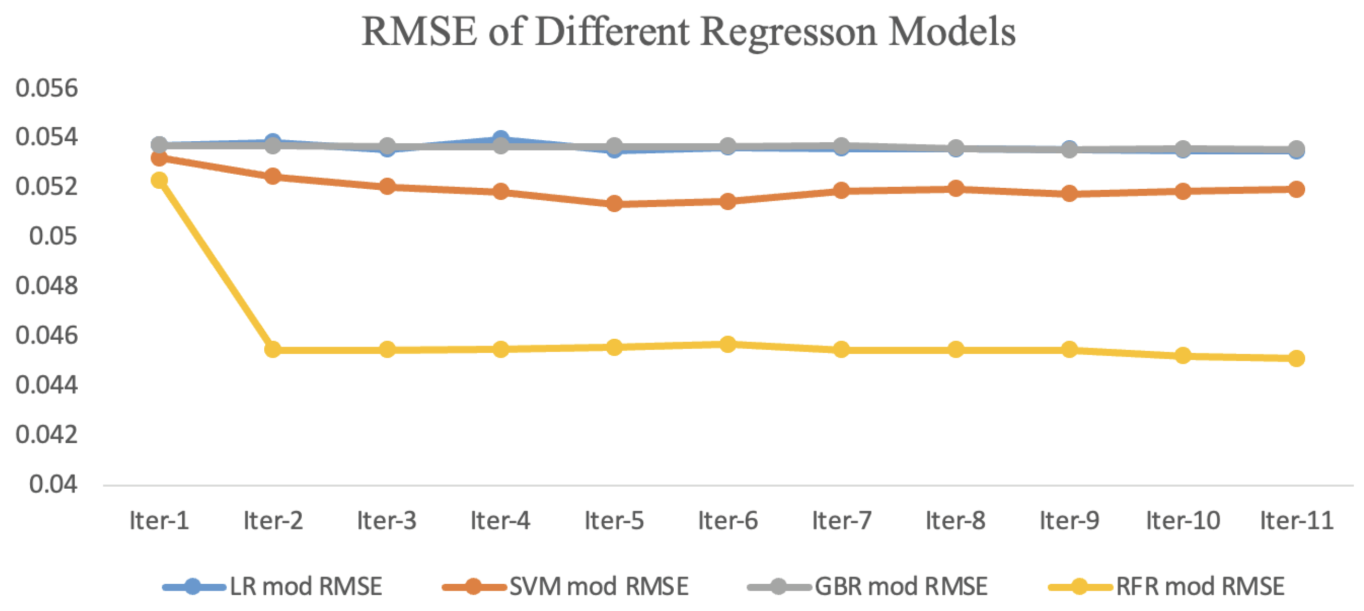
4.2. Self-Training Evaluation: Proposed Iterative Scheme for Semi-Supervised Learning

As explained earlier in Section 3.4.2, during Step 1 of the first iteration of the self-training for semi-supervised learning, the base learner is essentially the same as a model trained on the merged labeled data via supervised learning. For example—when the base learner is the LR model, then in Step 1, the first iteration of semi-supervised self-training (e.g., the beginning of self-training), the base learner is essentially the same as the benchmark model presented in Section 4.1. As described in Section 3.5.2, we perform three tests (Manifold Assumption: Iterative Error Test, Smoothness Assumption: Scatter Plot Test, and Smoothness Assumption: RMSE Approximate) on each model (LR, SVR, RFR, and GBR) to validate the predictions made by the models on the dataset from the human expert, D E x p e r t . This allows us to determine which is the best regression model for this dataset. Next, since LR and RFR are the only models that can provide feature importance, we use the best-performing model among LR and RFR to carry out the investigation with D E x p e r t , D P o s s i b l e , and D C o m p E x .
Smoothness Assumption, Scatter Plot Test for the LR Self-training, One Iteration: Two of the validation tests we perform on the semi-supervised models is to check whether the smoothness assumption holds or not. As mentioned in Section 3.5.2, one of these two is the scatter plot test, where we compare s c a t t e r P l o t D Y U L A , U , D X U L A , U with s c a t t e r P l o t D Y L A , D X L A to ensure that the distance between the feature vectors translates to the distance between prediction labels. For both datasets, we find that both plots show a positive trend. Based on characteristics displayed by the T T dataset in Figure 7, we also learn that feature vectors that are anywhere between 2 to Figure 8 arbitrary distance units from each other tend to have ORP values that are between 0.000 and 0.001 arbitrary distance units of one another. Most of the observations in the query set also follow this distance range pattern; however, the query also displays some outliers (those above the orange dotted line) that violate the distance range pattern. As such, the predictive pseudo-labels for these deviants inspire low confidence and are accordingly flagged. This process is repeated during each iteration.
Smoothness Assumption, RMSE Approximate for the LR Self-training, One Iteration: The RMSE of the test and query data are calculated as described in Section 3 for each model and dataset. For brevity, we show a sample for the LR model trained on the DExpert.The RMSE of LR on the training data is 0.0541, and on T T is 0.0539 (Figure 6). The calculated RMSE on the query dataset is 0.027. Since 0.027 falls in the [0.0, 0.054] range (Figure 7), at this stage, we accept the pseudo-labels as is without adding additional warning flags.
Manifold Assumption, Iterative Error Test, All Models: In this section, we check for random jumps in the RMSE values of the LR, RFR, SVR, and GBR models trained on D E x p e r t . As seen in Figure 8, the RMSE values for most of the models remain constant through all the iterations, illustrating that the addition of the query data points during each iteration is not violating the manifold assumption of semi-supervised learning. Thus, at this point in our analysis, we decided not to exclude any of the observations from the query sets since they all passed at least one of the smoothness assumptions tests and the manifold assumption.
Linear versus Non-linear Models, Feature Set Selection: Additionally, from Figure 8, we observe that all the non-linear regression models outperformed the linear regression model., with RFR achieving the best RMSE value of 0.046 and the GBR model obtaining a slightly better RMSE of 0.0532. This allows us to conclude that there is indeed non-linearity present in the dataset. Given that RFR achieves the lowest RMSE, we use RFR self-trained models for the next stage of the investigation. For comparison purposes, we also present the results obtained from LR self-trained model. At this stage, we investigate the effect of changing feature sets on the predictive performance of the models (Figure 9). Figure 9 shows the self-training iterations for the RFR and LR models on all three datasets, D E x p e r t , D P o s s i b l e , D C o m p E x . The RFR model performs best on all three datasets achieving the best performance with D C o m p E x (closely followed by D P o s s i b l e ). On the other hand, the iteratively self-trained LR model performs best with the D P o s s i b l e dataset, followed closely by D C o m p E x . This shows that the LR model, which can only recognize linear patterns, is not well suited to work with variables that may be important but presents a non-linear pattern in the data.

5. Discussion

5.1. Inference from the Supervised, Linear Model

A detailed result of the regression coefficients is depicted in Figure 10. Since 1 e y transformation was used for the target variable, each coefficient must be interpreted as an inverse relationship. Based on Figure 10, this LR benchmark shows that with the increase in the household size, people’s risk-taking will also increase by 0.44%. In other words, people will be 0.44% less risk averse, which is significant at the usual 1% tolerance. As income increases, risk-taking also increases by 0.25% (p-value: 0.000). Also, as people get older, they are 2.28% (p-value: 0.000) more risk-averse, which is in line with past literature [25]. Moreover, females are 0.93% (p-value: 0.000) more risk-averse than males, which is in line with the findings of [5].
On the other hand, according to the benchmark model, unemployed are 0.80% (p-value: 0.000) more risk averse than the individuals who are employed full time, which is also observed by Grable (2000). Compared to Asians, it is seen that Europeans are 0.88% (p-value: 0.000) more risk averse, Africans are 0.04% (p-value: 0.532) less risk averse, North Americans are 0.67% (p-value: 0.000) more risk averse, South Americans are 0.68% (p-value: 0.000) less risk averse. The heterogeneity in risk preferences across countries has been well documented in the literature, for example, refs. [12,26], although most research has compared European countries with North American countries.
Compared to Catholics, it is seen that Protestants are 0.50% (p-value: 0.000) less risk averse, Secular are 0.15% (p-value: 0.061) less risk averse, Muslims are 0.52% (p-value: 0.000) less risk averse, Hinduisms are 1.14% (p-value: 0.000) more risk averse. Past research has found mixed results on the effect of religion on risk aversion. While [27] find that Protestants are more risk-averse or make safer financial investments than Catholics, refs. [28,29] find the opposite. Compared to the individuals who have completed primary education (or less), individuals who have at least some secondary education are 0.90% (p-value: 0.000) less risk averse, and individuals with college (or higher) degrees are 1.59% (p-value: 0.000) less risk averse. This is in line with [12], who finds that individuals with low cognitive skills are more risk-averse.

5.2. Inference from the Semi-Supervised, Non-Linear Model

Since this paper finds that the LR model is not well suited, it refrains from interpreting the linear coefficients; rather, it discusses the importance of the variables taking into consideration the non-linear relationships.
The results (Figure 5) indicate that demographic characteristics are important determinants of an individual’s willingness to take a risk. This paper finds age and being female are important determinants of willingness to take a risk. Past literature has also shown that women and the old are substantially more risk-averse than men and young people [25,29,30].
The findings in Figure 11 show that education explains about 9% of the willingness to take a risk variation. Past research finds that people with low skills are also found to be risk-averse [12]. But most of this research uses a continuous variable for skills or looks at the quality of education rather than just the indicator variable as we do.
Various other studies have shown that geographic and cultural factors also explain preferences. For example, ref. [12] show that family structure, income level, and crop suitability of land matter at the country level. Results in Figure 11 reveal that being married explains about 3%, while the continent or region dummies explain about 8% of the variation in risk aversion.
Religion dummies explain about 9% of the variation in risk preference. Protestantism and patience or time preference have long been linked to capitalism’s rise [15,31]. More recently, ref. [32] have shown that religiousness is an important determinant of risk aversion. Findings suggest that religious persons are less risk-tolerant than atheists, and Muslims are less risk tolerant than Christians in Germany. Research has also shown that there is a substantial difference in risk preference between migrants and natives [33], with non-economic migrants in Germany being more risk averse than natives and this gap across employment status, gender, and skills, while economic migrants risk preference is almost the same as native. Our results support these findings as we find that the migrants’ dummy does not explain risk preference significantly.
Health feature explains about 3% of the variation in risk preference. The impact of physical health-related problems on risk preference has been addressed in a few pieces of research, which find a positive relationship between willingness to take a risk and good health [34,35]. We also found that healthy people are also less risk averse, e.g., their risk-taking tendency is higher than their counterparts.
Ref. [36] theoretically shows relative deprivation as a cause of risky behavior and shows that an individual’s relative risk aversion decreases as he becomes more relatively deprived. Subjective well-being measures, as reported by the Gallup World Poll survey, provide a proxy for relative deprivation felt by the individual. The third column in Figure 5 reveals the empirical importance of subjective well-being or feeling of deprivation on risk aversion and the importance of the variables already pointed out in past literature. For example, the optimistic feature explains about 3% of the variation in risk preference. The categorical variable is created based on the question “Life in 5 Years”, with reactions of respondents being answered on a Likert scale ranging from worst possible to best possible. It is found that individuals with an optimistic view are significantly less risk-averse.
The social network feature explains about 3% of the variation in risk preference. This binary variable is generated from the question “Count on to help”, and the responses were affirmative or negative. It is also found that individuals with socially helpful attitudes are significantly less risk-averse.
The corruption feature also explains about 3% of the variation in risk preference. From a binary response type question “Corruption Within Businesses” this feature is created. It is also found that individuals facing corruption in their business are significantly less risk averse.

6. Conclusions

Numerous studies have explored the determinants influencing individuals’ inclination towards general and financial risks, often centering on the relationships between sociodemographic, economic variables, and self-reported risk attitudes. However, to the best of our knowledge, no prior study has employed a semi-supervised machine learning algorithm approach to predict an individual’s observed intention to accept general risks, particularly in scenarios where the observed risk variable is absent.
This research innovatively combines a semi-supervised method with econometric tools to forecast individuals’ willingness to undertake general risks, utilizing observed risk preferences and their social, economic, and demographic profiles, drawing from the merged Gallup and GPS dataset. Through this approach, we successfully predicted missing observed risk values in the Gallup dataset for the years 2006–2011 and 2013–2018. Rigorous evaluations, employing both traditional machine learning techniques and our proposed iterative evaluation scheme, ensured the quality of predictions extended beyond 2012.
Our findings challenge the adequacy of linear models in studying risk and associated factors. Notably, well-being indicators such as the optimism index, social network, good health, and corruption index emerged as potentially influential in individuals’ risk-taking decisions. While further investigations are warranted to establish causation and enhance confidence in these results, our study provides compelling evidence to advocate for a more comprehensive approach to studying risk-taking.
A limitation of our current study lies in its exclusive use of self-training semi-supervised techniques for ORP predictions. Future endeavors aim to employ diverse machine learning methods, including semi-supervised techniques such as wrapper methods and graph-based methods, as well as weak-supervised techniques, to further refine and expand our predictive capabilities.

Author Contributions

M.S. provided data. M.S., R.S., F.A. and T.S. designed the data and drafted the manuscript. M.S. and R.S. acted in supervisory role throughout. All authors have read and agreed to the published version of the manuscript.

Funding

This research received no external funding.

Data Availability Statement

The Gallup World Poll is not publicly available and can be bought from Gallup. United Arab Emirates University had subscription of the data and Dr. Mrittika Shamsuddin, one of the authors accessed the data when she was appointed as an Assistant Professor at United Arab Emirates University in 2018 and consequently our data ends it that year.

Acknowledgments

We thank Mohammad Tareque, the Director at Bangladesh Institute of Governance and Management (BIGM), for his support and guidance and making resources available for this research.

Conflicts of Interest

There are no conflicts of interest.

Abbreviations

The following abbreviations are used in this manuscript:
D1GPS data with ORP for the year 2012
D2Gallup data for the year 2012
D3Gallup data without ORP for the year 2005–2011, 2013–2018
TLORPTrue Label ORP
PORPTPredicted ORP on labeled test set
PPORPQPredicted Pseudo ORP from query data (PPORPQ)

Appendix A

Here we answer how the risk-preference index is calculated in GPS dataset [12]. The risk-preference index in GPS is calculated by weighing the qualitative question by 0.527 and the quantitative questions by 0.473. The quantitative survey measure consists of a series of five interdependent hypothetical binary choices. Choices were between a fixed lottery, in which the individual could win x or zero, and varying sure payments, y. The exact question is the following: Please imagine the following situation. You can choose between a sure payment of a particular amount of money, or a draw, where you would have an equal chance of getting the amount x or getting nothing. We will present to you five different situations. What would you prefer: a draw with a 50. The sure payment was increased gradually in the following questions to identify an individual’s certainty equivalence. The sequence of questions follows as the first being, and each respondent was asked whether they would prefer to receive EUR 160 for sure or whether they preferred a 50:50 chance of receiving EUR 300 or nothing. If the respondent opted for the safe choice (“B”), the safe amount of money offered in the second question decreased to EUR 80. If, on the other hand, the respondent opted for the gamble (“A”), the safe amount was increased to EUR 240, and this continued for five turns. If the individual chooses B on each of the terms, his willingness to take a risk is given the number 1, while the individual takes the gamble in each of the five rounds, and his willingness to take a risk is given the number 32. The qualitative item asks for the respondents’ self-assessment of their willingness to take risks on an 11-point scale, which is more common in the literature [8]. Thus, the risk preference index in GPS contains more information than the self-reported binary indicator for willingness to take risks.
As explained in Section 3.6, there are three feature sets (Figure 5):
  • D E x p e r t —this feature set is based on the subject expert’s knowledge and experience in general risk-taking
  • D P o s s i b l e —this feature set includes all the features that could be included from the merged dataset (Figure 2).
  • D C o m E x 
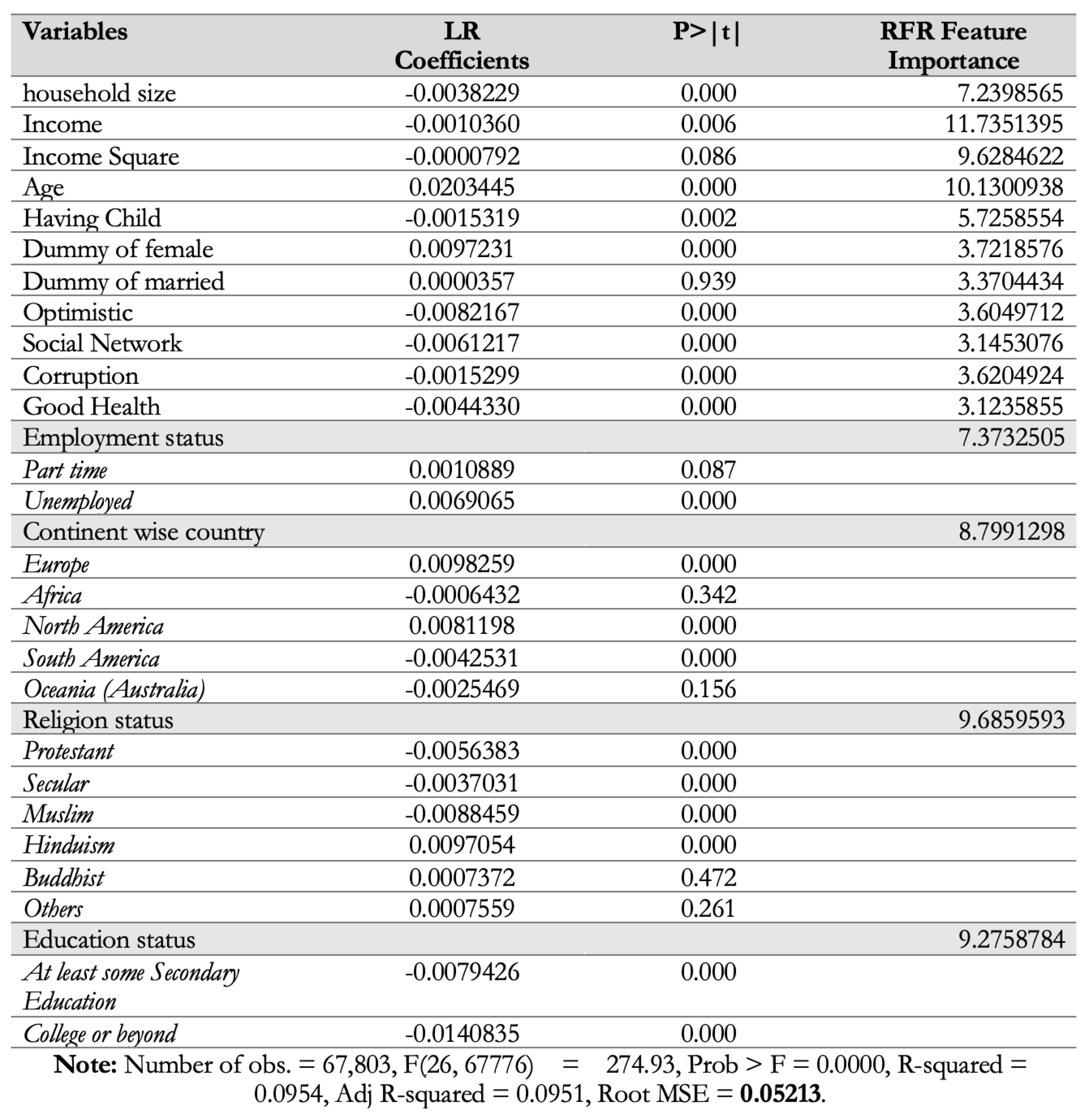
—this feature set is a proper subset of DPossible, which consists of features that were either found to be significantly important by the LR or given high importance by the RFR. The resulting feature sets are provided in Figure 5, while Figure 11 provides more details about the feature importance obtained for the D C o m E x dataset by the RFR (Column 4), along with the coefficients and p-values from the LR model trained on D C o m E x (Columns 2 and 3).

References

  1. Dohmen, T.; Quercia, S.; Willrodt, J. Willingness to Take Risk: The Role of Risk Conception and Optimism. In IZA Discussion Paper; IZA: Bonn, Germany, 2018; p. 11642. [Google Scholar]
  2. Dohmen, T.; Wagner, G.G. ROA Individual Risk Attitudes: Measurement, Determinants and Behavioral Consequences Individual Risk Attitudes: Measurement, Determinants and Behavioral Consequences. J. Eur. Econ. Assoc. 2009, 9, 522–550. [Google Scholar] [CrossRef]
  3. Frey, R.; Pedroni, A.; Mata, R.; Rieskamp, J.; Hertwig, R. Risk preference shares the psychometric structure of major psychological traits. Sci. Adv. 2017, 3, e1701381. [Google Scholar] [CrossRef]
  4. Pedroni, A.; Frey, R.; Bruhin, A.; Dutilh, G.; Hertwig, R.; Rieskamp, J. The risk elicitation puzzle. Nat. Hum. Behav. 2017, 1, 803–809. [Google Scholar] [CrossRef]
  5. Falk, A.; Becker, A.; Dohmen, T.J.; Enke, B.; Huffman, D.; Sunde, U. The Nature and Predictive Power of Preferences: Global Evidence; Centre for Economic Policy Research: London, UK, 2015. [Google Scholar]
  6. Browne, M.J.; Jäger, V.; Richter, A.; Steinorth, P. Family changes and the willingness to take risks; African Americans. Bioinformatics 2018, 27, 1384–1389. [Google Scholar]
  7. Dohmen, T.; Falk, A.; Huffman, D.; Sunde, U. The intergenerational transmission of risk and trust attitudes. In IZA Discussion Papers; IZA: Bonn, Germany, 2006; Available online: https://docs.iza.org/dp2380.pdf (accessed on 7 March 2024).
  8. Dohmen, T.; Falk, A.; Huffman, D.; Sunde, U. The intergenerational transmission of risk and trust attitudes. Rev. Econ. Stud. 2012, 79, 645–677. [Google Scholar] [CrossRef]
  9. Azar, S.A. Measuring relative risk aversion. Appl. Financ. Econ. Lett. 2006, 2, 341–345. [Google Scholar] [CrossRef]
  10. Outreville, J.F. Risk Aversion, Risk Behavior, and Demand for Insurance: A Survey. J. Insur. Issues 2014, 37, 158–186. [Google Scholar] [CrossRef]
  11. Hareli, S.; Elkabetz, S.; Hanoch, Y.; Hess, U. Social perception of risk-taking willingness as a function of expressions of emotions. Front. Psychol. 2021, 12, 655314. [Google Scholar] [CrossRef]
  12. Falk, A.; Becker, A.; Dohmen, T.; Enke, B.; Huffman, D.; Sunde, U. Global Evidence on Economic Preferences. Q. J. Econ. 2018, 133, 1645–1692. [Google Scholar] [CrossRef]
  13. Grable, J.E. Financial risk tolerance and additional factors that affect risk taking in everyday money matters. J. Bus. Psychol. 2000, 14, 625–630. [Google Scholar] [CrossRef]
  14. Yao, R.; Gutter, M.S.; Hanna, S.D. The financial risk tolerance of Blacks, Hispanics and Whites. J. Financ. Couns. Plan. 2005, 16, 51–62. [Google Scholar]
  15. Schneider, C.R.; Fehrenbacher, D.D.; Weber, E.U. Catch me if I fall: Cross-national differences in willingness to take financial risks as a function of social and state ‘cushioning’. Int. Bus. Rev. 2017, 26, 1023–1033. [Google Scholar] [CrossRef]
  16. Zhu, X. Semi-Supervised Learning Literature Survey; Technical Report, Computer Sciences; University of Wisconsin-Madison: Madison, WI, USA, 2005. [Google Scholar]
  17. Van Engelen, J.E.; Hoos, H.H. A survey on semi-supervised learning. Mach. Learn. 2020, 109, 373–440. [Google Scholar] [CrossRef]
  18. Belgiu, M.; Drăguţ, L. Random forest in remote sensing: A review of applications and future directions. ISPRS J. Photogramm. Remote. Sens. 2016, 114, 24–31. [Google Scholar] [CrossRef]
  19. Segal, M.R. Machine Learning Benchmarks and Random Forest Regression; UCSF: San Francisco, CA, USA, 2004. [Google Scholar]
  20. Kolarik, N.; Shrestha, N.; Caughlin, T.; Brandt, J. Leveraging high resolution classifications and random forests for hindcasting decades of mesic ecosystem dynamics in the Landsat time series. Ecol. Indic. 2024, 158, 111445. [Google Scholar] [CrossRef]
  21. Myles, A.J.; Feudale, R.N.; Liu, Y.; Woody, N.A.; Brown, S.D. An introduction to decision tree modeling. J. Chemom. J. Chemom. Soc. 2004, 18, 275–285. [Google Scholar] [CrossRef]
  22. Ardabili, S.; Mosavi, A.; Várkonyi-Kóczy, A.R. Advances in machine learning modeling reviewing hybrid and ensemble methods. In Engineering for Sustainable Future: Selected Papers of the 18th International Conference on Global Research and Education Inter-Academia–2019; Springer: Berlin/Heidelberg, Germany, 2020; Volume 18, pp. 215–227. [Google Scholar]
  23. Awad, M.; Khanna, R.; Awad, M.; Khanna, R. Support vector regression. In Efficient Learning Machines: Theories, Concepts, and Applications for Engineers and System Designers; Springer: Berlin/Heidelberg, Germany, 2015; pp. 67–80. [Google Scholar]
  24. Hepp, T.; Schmid, M.; Gefeller, O.; Waldmann, E.; Mayr, A. Approaches to regularized regression—A comparison between gradient boosting and the lasso. Methods Inf. Med. 2016, 55, 422–430. [Google Scholar] [CrossRef]
  25. Veider, F.M.; Lefebvre, M.; Bouchouicha, R.; Chmura, T.; Hakimov, R.; Krawczyk, M.; Martinsson, P. Common Components of Risk and Uncertainty Attitudes across Contexts and Domains: Evidence from 30 Countries. J. Eur. Econ. Stat. 2015, 13, 421–452. [Google Scholar] [CrossRef]
  26. Vollenweider, X.; Di Falco, S.; O’Donoghue, C. Risk Preferences and Voluntary Agri-Environmental Schemes: Does Risk Aversion Explain the Uptake of the Rural Environment Protection Scheme? Grantham Research Institute: London, UK, 2011. [Google Scholar]
  27. Kumar, A.; Page, J.K.; Spalt, O.G. Religious Beliefs, Gambling Attitudes and Financial Market Outcomes. J. Financ. Econ. 2011, 102, 671–708. [Google Scholar] [CrossRef]
  28. Renneboog, L.; Spaenjers, C. Religion, Economic Attitudes, and Household Finance. Oxf. Econ. Pap. 2012, 64, 103–127. [Google Scholar] [CrossRef]
  29. Dohmen, T.; Falk, A.; Huffman, D.; Sunde, U.; Schupp, J.; Wagner, G.G. Individual Risk Attitudes: Measurement, Determinants, and Behavioral Consequences. J. Eur. Assoc. 2011, 9, 522–550. [Google Scholar] [CrossRef]
  30. Croson, R.; Gneezy, U. Gender Differences in Preferences. J. Econ. Lit. 2009, 47, 448–474. [Google Scholar] [CrossRef]
  31. Weber, C. A modification of Sakaguchi’s reaction for the quantitative determination of arginine. J. Biol. Chem. 1930, 86, 217–222. [Google Scholar] [CrossRef]
  32. Bartke, S.; Schwarze, R. Risk Averse by Nation or by Religion? Some Insights on the Determinants of Individual Risk Attitudes. SOEPpaper 2008. [Google Scholar] [CrossRef]
  33. Deole, S.S.; Rieger, M.O. The immigrant-native gap in risk and time preferences in Germany: Levels, socio-economic determinants, and recent changes. J. Popul. Econ. 2023, 36, 743–778. [Google Scholar] [CrossRef]
  34. Schurer, S. Lifecycle patterns in the socioeconomic gradient of risk preferences. J. Econ. Behav. Organ. 2015, 119, 482–495. [Google Scholar] [CrossRef]
  35. Bascans, J.M.; Courbage, C.; Oros, C. Means-tested public support and the interaction between long-term care insurance and informal care. Int. J. Health Econ. Manag. 2017, 17, 113–133. [Google Scholar] [CrossRef] [PubMed]
  36. McKune, S.L.; Stark, H.; Sapp, A.C.; Yang, Y.; Slanzi, C.M.; Moore, E.V.; Omer, A.; Wereme N’Diaye, A. Behavior change, egg consumption, and child nutrition: A cluster randomized controlled trial. Pediatrics 2020, 146, e2020007930. [Google Scholar] [CrossRef] [PubMed]
Figure 1. An overview of the research methodology used to predict ORP values for the Gallup data.
Mca 29 00021 g001
Figure 2. An overview of the data usage and the contributions of this research work.
Mca 29 00021 g002
Figure 3. Overview of the evaluation schemes used to evaluate the benchmark and semi-supervised models.
Mca 29 00021 g003
Figure 4. A schematic overview of the self-training semi-supervised learning mechanism using base learners. These base learners can be linear (e.g., find linear patterns only) or non-linear models (e.g., finds linear and non-linear patterns).
Mca 29 00021 g004
Figure 5. Feature sets for D E x p e r t , D P o s s i b l e , D C o m p E x .
Mca 29 00021 g005
Figure 6. Benchmark LR Model Evaluation. Independent variables are chosen by the human expert.
Mca 29 00021 g006
Figure 7. Scatter plot comparison for LR Self-training, first iteration, Step 1 (left) and Step 2 (right). This particular figure uses the D E x p e r t dataset.
Mca 29 00021 g007
Figure 8. The RMSE values of the four ML regression models over the ten iterations of the self-training stage plus the initially supervised base learner.
Mca 29 00021 g008
Figure 9. The performance of the LR and RFR model on the three datasets, D E x p e r t , D P o s s i b l e , D C o m p E x . The best regression prediction is by RFR on D C o m p E x .
Mca 29 00021 g009
Figure 10. Benchmark LR Model coefficients for the merged data from the year 2012.
Mca 29 00021 g010
Figure 11. Detailed coefficients of base learner based on computational expert features.
Mca 29 00021 g011
Table 1. The various variable transformation combinations that were used to run empirical experiments to find the combination that satisfied the assumptions of OLS regression.
VariableTransformation
Willingness to take a risk (risk-taking) 1 y , 1 e y , 1 y 2 , 1 y
Age ln ( x ) , x 2
GenderBinary
Marital statusBinary
Income per capita ln ( x ) , x 2
Income per capita square ln ( x ) , x 2
Education levelBinary
Household size ln ( x ) , x 2
Having ChildBinary
ReligionBinary
Employment statusBinary
Residence statusBinary
Migration statusBinary
Continent of respondentBinary
RemittanceBinary
Disclaimer/Publisher’s Note: The statements, opinions and data contained in all publications are solely those of the individual author(s) and contributor(s) and not of MDPI and/or the editor(s). MDPI and/or the editor(s) disclaim responsibility for any injury to people or property resulting from any ideas, methods, instructions or products referred to in the content.

