Curve and Surface Construction Using Hermite Trigonometric Interpolant

Abstract

In this paper, the constructions of both open and closed trigonometric Hermite interpolation curves while using the derivatives are presented. The combination of tension, continuity, and bias control is used as a very powerful type of interpolation; they are applied to open and closed Hermite interpolation curves. Surface construction utilizing the studied trigonometric Hermite interpolation is explored and several examples obtained by the ${\mathcal{C}}^1$ trigonometric Hermite interpolation surface are given to show the usefulness of this method.

1. Introduction

Parametric curves that are used in computer graphics are normally based on polynomials, which is reasonable, since polynomials are simple functions that are easy to calculate and flexible enough to create many different shapes. However, in principle, different types of functions can be used to develop a parametric curve or surface. These methods are based on control points. While using polynomials, it will be easy to construct a parametric curve segment (or surface patch) that passes through a given one-dimensional array or two-dimensional grid of points, respectively. The downside of these methods is that they are not interactive. Charles Hermite developed a way to smoothly interpolate any mathematical quantity from an initial value to a final value, given the rates of change of the quantity at the start and end, and he then derived its blending functions. Hermite curves are very powerful and also very easy to calculate. The mathematical background of Hermite curves is an important tool that helps to understand the entire family of splines. For example, the Catmull–Rom spline [1] is just a subset of the cardinal splines and they are really great to smoothly interpolate between a set of data. A special form of the Hermite curves is the so called KB-splines, curves with control over tension, continuity, and bias. Kochanek and Bartels introduced these curves in 1984 [2] to give animators more control over keyframe animation. They introduced three control-values for each keyframe point: the tension parameter shows how sharply the curve bends, the continuity parameter illustrates how rapid the change in speed and direction is, and the bias controls the direction of the curve as it passes through the keypoint. Several authors have published the Hermite trigonometric interpolation problem. For example, Barrera et al. [3] presented a method that can be used to obtain minimal bending trigonometric Hermite curves. These curves can be used in a number of areas, such as three-dimensional (3D)-modeling and camera movements. In [4], Han presented explicit piecewise trigonometric Hermite interpolation methods that are based on the symmetric, nonnegative, and normalized basis of trigonometric polynomials. These trigonometric Hermite interpolants are local and easy to compute. In the last decade, many studies have been conducted on rectangular interpolation; for example, in [5], they reported rational interpolants with tension parameters and extended their method to the rectangular topology case. Zhang and Wang [6] presented a new way for constructing ${\mathcal{C}}^2$ quartic spline interpolation surface, which makes the curve/surface formed to have the same advantages as cubic spline curve/surface in having a simple construction and being easy to compute. In [7], the authors developed a bivariate rational Hermite interpolation in order to create a space surface using both function values and the first-order partial derivatives of the function being interpolated as the interpolation data. Fang et al. [8] studied a method of rectangular interpolation of a given 3D data array that is regularly arranged. They constructed ${\mathcal{C}}^2$ and ${\mathcal{C}}^3$ interpolating spline surfaces while using tensor product; it has desirable properties and it is easily implemented and adjusted. Juncheng presented a class of trigonometric cubic Hermite interpolating curves with a shape parameter [9]. In [10], Akima presented a method of bivariate interpolation and smooth surface fitting based on local procedures, after that Dodd et al. [11] made an improvement of Akima’s method and reported a technique for smooth surface interpolation over grid data in order to reduce the number of extraneous local optima and inflection points of the surface. Zhang [12] studied an extension of cubic curves (C-curves) using the basis $sint$, $cost$, t, and 1. The curves depend on one positive parameter. He showed that these curves can deal with circular arcs, cylinders, cones, and toruses. Recently, Li [13] and Li et al. [14] proposed a class of trigonometric interpolation curves with two parameters that can interpolate some given data points without solving equation systems. They are also ${\mathcal{C}}^2$ and they have two degrees of freedom in the interpolation curves and, thus, can adjust their shape by altering the values of the two parameters. More recently, BiBi et al. constructed various shapes and font designing of curves and described the curvature by using parametric and geometric continuity constraints of generalized hybrid trigonometric Bézier (GHT-Bézier) curves [15]. In another very recent work, Usman et al. [16] presented a new TC Bernstein-like basis functions analogous to standard Bernstein basis functions with single shape parameter to overcome the drawing of complex curves. They constructed some conic curves by choosing appropriate points and some complex curves by using continuity conditions. Even with the existence of polynomial Hermite interpolant, the problem of inaccurate approximation always remains for some types of curves, such as arcs, helix, cycloid, catenary, and the exponential curves. In order to avoid their shortcomings, in this work we propose the trigonometric Hermite interpolant, which is a mixture of cosine, sine, and $\{1,x\}$ used in [6]. This interpolant gives more advantages and accurate approximation. The curves and surfaces, most commonly used in computer-assisted design, or even in engineering applications, are often helixes, cycloids, arcs, cylinders, or spheres. Thus, polynomial Hermite interpolant does not always give good approximations, so it is necessary to find splines in order to overcome this disadvantage. This paper reports a new mixture of polynomial and trigonometric functions, combined with tension, continuity, and bias control, to build the new Hermite interpolant. This Hermite interpolation allows the animator to change the tension, continuity, and bias of these splines. They are used to smoothly interpolate data between key-points like object movement in keyframe animation or camera control. One of the benefits of this combination is the adjustments to overcome speed discontinuities. The curves and surfaces, most commonly used in computer-assisted design or even in engineering applications, are often helixes, cycloids, arcs, cylinders, or spheres. Thus, the use of polynomial Hermite interpolant does not always give good approximations, so it is necessary to find new splines in order to overcome this disadvantage. In this paper, we report new mixture of polynomial and trigonometric functions to build a new Hermite interpolant. This Hermite interpolation leads to the construction of a new and interesting trigonometric Hermite basis having the same properties as the classical basis of Hermite polynomials. Tension, continuity, and bias control were combined and used as a very powerful type of interpolation.

The paper is structured, as follows. In Section 2, a trigonometric Hermite spline interpolation is developed and trigonometric Hermite basis functions are constructed. Section 3 deals with the construction of open and closed trigonometric Hermite interpolation curves using the derivatives, which are illustrated by some examples. Section 4 introduces a powerful type of interpolation using Tension, Continuity, and Bias parameters. A combination of these three parameters is applied to open and closed Hermite interpolation curves, and the influence of each parameter on the interpolation curve is exihibited through examples. In Section 5, we provide the construction of a spline interpolation surface using our trigonometric Hermite basis. Several examples are given to show the usefulness of this method. Finally, Section 6 summarizes our findings.

2. Trigonometric Hermite Spline Interpolation

In this section, we develop the trigonometric Hermite spline interpolation. To do this, we consider the uniform grid partition:

$$\Delta =\{0=x_0<x_1<\dots <x_{n-1}<x_n=\frac{\pi }{2}\}$$

of the interval $I=[0,\frac{\pi }{2}]$, where $x_i=ih,0\le i\le n,$ and $h=\frac{\pi }{2n}$. At the knots of $\Delta$, the values $f\left(x_i\right)$ and $f^{\prime }\left(x_i\right)$, $i=0,\dots ,n-1,$ which are supposed to come from an unknown differentiable function f, are given. We denote, by ${\mathcal{S}}^1(\Delta ,I)$, the space of trigonometric splines of class ${\mathcal{C}}^1$, defined by:

$$\begin{array}{c}\hfill {\mathcal{S}}^1(\Delta ,I)=\{s\in {\mathcal{C}}^1\left(I\right):s_{{|}_{[x_i,x_{i+1}]}}\in \Gamma ,i=0,\dots ,n-1\}\end{array}$$

(1)

where $\Gamma =span\{1,x,sin(x),cos(x\left)\right\}$.

More precisely, we can define the following trigonometric Hermite spline interpolation problem.

Problem: Given $2n$ interpolation values

$$\begin{array}{cc}\hfill f^{\left(r\right)}\left(x_i\right),& i=0,\dots ,n-1,r=0,1\end{array}$$

(2)

find $s\in {\mathcal{S}}^1(\Delta ,I)$ such that

$$\begin{array}{cc}\hfill s^{\left(r\right)}\left(x_i\right)=f^{\left(r\right)}\left(x_i\right),& i=0,\dots ,n-1,r=0,1.\end{array}$$

(3)

Theorem 1.

There exists a unique spline $s\in {\mathcal{S}}^1(\Delta ,I)$, which satisfies the interpolatory conditions (3). This spline can be written, as follows: $\forall x\in [x_i,x_{i+1}[$

$$s_i\left(x\right)=a_{0,i}+a_{1,i}x+a_{2,i}sin\left(x\right)+a_{3,i}cos\left(x\right),$$

(4)

where

$$\begin{array}{cc}\hfill a_{0,i}& =C_h(f^{\prime }\left(x_i\right)\left(-cos\left(h\right)\left(x_{i+1}\right)+sin\left(h\right)+x_i\right)+f^{\prime }\left(x_{i+1}\right)\left(-cos\left(h\right)x_i+h-sin\left(h\right)+x_i\right)\hfill \\ \hfill & +f\left(x_{i+1}\right)\left(-sin\left(h\right)x_i+cos\left(h\right)-1\right)+f\left(x_i\right)\left(sin\left(h\right)\left(x_{i+1}\right)+cos\left(h\right)-1\right)),\hfill \\ \hfill a_{1,i}& =C_h(-2sin(\frac{h}{2})(sin(\frac{h}{2})(f^{\prime }(x_{i+1})+f^{\prime }(x_i))+cos(\frac{h}{2})\left(f\left(x_i\right)-f\left(x_{i+1}\right))\right),\hfill \\ \hfill a_{2,i}& =C_h(f^{\prime }\left(x_i\right)\left(hsin\left(x_{i+1}\right)+cos\left(x_{i+1}\right)-cos\left(x_i\right)\right)-f^{\prime }\left(x_{i+1}\right)\left(hsin\left(x_i\right)+cos\left(x_{i+1}\right)-cos\left(x_i\right)\right)\hfill \\ \hfill & +f\left(x_{i+1}\right)\left(sin\left(x_i\right)-sin\left(x_{i+1}\right)\right)+f\left(x_i\right)\left(sin\left(x_{i+1}\right)-sin\left(x_i\right)\right)\left)\right),\hfill \\ \hfill a_{3,i}& =C_h(f^{\prime }\left(x_i\right)\left(-sin\left(x_{i+1}\right)+hcos\left(x_{i+1}\right)+sin\left(x_i\right)\right)+f^{\prime }\left(x_{i+1}\right)\left(sin\left(x_{i+1}\right)-hcos\left(x_i\right)-sin\left(x_i\right)\right)\hfill \\ \hfill & +f\left(x_i\right)\left(cos\left(x_{i+1}\right)-cos\left(x_i\right)\right)+f\left(x_{i+1}\right)\left(cos\left(x_i\right)-cos\left(x_{i+1}\right)\right)\left)\right),\hfill \end{array}$$

with $C_h=\frac{1}{{sin}^2\left(\frac{h}{2}\right)\left(2hcot\left(\frac{h}{2}\right)-4\right)}$.

Proof. 

Let $s_i\left(x\right)=a_{0,i}+a_{1,i}x+a_{2,i}sin\left(x\right)+a_{3,i}cos\left(x\right),\forall x\in [x_i,x_{i+1}[$. The coefficients $a_{j,i},j=0,\dots ,3$ must be chosen, so that $s_i\left(x\right)$ will interpolate f and $f^{\prime }$ at $x_i$ and $x_{i+1}$. This is equivalent to the following linear system

$$\begin{array}{c}\hfill \left[\begin{array}{cccc}1& x_i& sin\left(x_i\right)& cos\left(x_i\right)\\ 0& 1& cos\left(x_i\right)& -sin\left(x_i\right)\\ 1& x_{i+1}& sin\left(x_{i+1}\right)& cos\left(x_{i+1}\right)\\ 0& 1& cos\left(x_{i+1}\right)& -sin\left(x_{i+1}\right)\end{array}\right]\left[\begin{array}{c}{a}_{0,i}\\ a_{1,i}\\ a_{2,i}\\ a_{3,i}\end{array}\right]=\left[\begin{array}{c}f\left(x_i\right)\\ f^{\prime }\left(x_i\right)\\ f\left(x_{i+1}\right)\\ f^{\prime }\left(x_{i+1}\right)\end{array}\right]\end{array}$$

It can be shown that the determinant of this system is

$$\left(x_{i+1}-x_i\right)sin\left(x_{i+1}-x_i\right)+2\left(cos\left(x_{i+1}-x_i\right)-1\right).$$

Therefore, the system has to be solvable under our assumptions that the abscissas $x_i=ih$ are distinct. □

3. Trigonometric Hermite Interpolation Curves

However, some applications require that the interpolant be such that not only the functional values are matched, but also the derivatives at the nodes. In this section, we consider the situation in which we also want to interpolate derivative information for constructing the interpolating curves.

Given the sequence of data points $P_i\in {\mathbb{R}}^2$, $i=0,\dots ,n-1$, along with associated strictly monotone parameter values $x_i=ih\in [0,\frac{\pi }{2}],$$i=0,\dots ,n-1$, with $h=\frac{\pi }{2(n-1)}$. In order to calculate derivatives, it is a natural idea to estimate the derivative at the point $P_i$ by the difference $P_{i+1}-P_i$ or $P_i-P_{i-1}$, and more rational estimate may be their average (see [1,2]). We now use the weighted average on neighboring positions of $P_i$ to generate these derivatives, noted $D_i$.

Now, if we put $D_i=\frac{1}{2}(P_{i+1}-P_{i-1}),$ then, according to the endpoints interpolation, it is known that ${\varphi }_0$ and ${\varphi }_1$ are determined by the values at the ends of the interval, and the derivatives determine ${\varphi }_2$ and ${\varphi }_3$ at the ends. Thus, it is natural to associate $P_i$ to ${\varphi }_0$, $P_{i+1}$ to ${\varphi }_1$, $D_i$ to ${\varphi }_2$ and $D_{i+1}$ to ${\varphi }_3$. Subsequently, the trigonometric Hermite interpolation curve is defined as

$$\begin{array}{ccc}\hfill C\left(x\right)& =& C_i\left(\frac{\pi }{2}\frac{x-x_i}{h}\right),x\in [x_i,x_{i+1}],\hfill \end{array}$$

(5)

where, $C_i\left(u\right)=P_i{\varphi }_0\left(u\right)+P_{i+1}{\varphi }_1\left(u\right)+\frac{2h}{\pi }{D}_i{\varphi }_2\left(u\right)+\frac{2h}{\pi }{D}_{i+1}{\varphi }_3\left(u\right)$, $u\in [0,\frac{\pi }{2}].$

We can rewrite this equation in the matrix form, as follows:

$$\begin{array}{c}\hfill C_i\left(u\right)={\left[\begin{array}{c}1\\ u\\ sin\left(u\right)\\ cos\left(u\right)\end{array}\right]}^T\left[\begin{array}{cccc}\frac{\pi -2}{\pi -4}& \frac{-2}{\pi -4}& \frac{2}{\pi -4}& \frac{\pi -2}{\pi -4}\\ \frac{-2}{\pi -4}& \frac{2}{\pi -4}& \frac{-2}{\pi -4}& \frac{-2}{\pi -4}\\ \frac{2}{\pi -4}& \frac{-2}{\pi -4}& \frac{\pi -2}{\pi -4}& \frac{2}{\pi -4}\\ \frac{-2}{\pi -4}& \frac{2}{\pi -4}& \frac{-2}{\pi -4}& \frac{2-\pi }{\pi -4}\end{array}\right]\left[\begin{array}{c}{P}_i\\ P_{i+1}\\ \frac{2h}{\pi }{D}_i\\ \frac{2h}{\pi }{D}_{i+1}\end{array}\right]\end{array}$$

Remark 1.

For the construction of closed trigonometric Hermite interpolation curves, it is sufficient to periodize the end control points and the knots, i.e., $P_n=P_0$ and $x_n=x_0$.

By means of formulas above, one can easily prove the next lemma.

Lemma 1.

The continuity of the trigonometric Hermite curve interpolant (5) is expressed, as follows:

$$\begin{array}{c}\hfill \left\{\begin{array}{c}C\left(x_i^{-}\right)=C\left(x_i^{+}\right)=P_i\hfill \\ C^{\prime }\left(x_i^{-}\right)=C^{\prime }\left(x_i^{+}\right)=D_i\hfill \end{array}\right.\end{array}$$

(6)

Proof. 

From (5) and according to simple calculations, we obtain:

$$\begin{array}{c}\hfill \left\{\begin{array}{c}{C}_i\left(0\right)=P_i\hfill \\ C_{i-1}\left(\frac{\pi }{2}\right)=P_i\hfill \\ C_i^{\prime }\left(0\right)=\frac{2h}{\pi }{D}_i\hfill \\ C_{i-1}^{\prime }\left(\frac{\pi }{2}\right)=\frac{2h}{\pi }{D}_i\hfill \end{array}\right.\end{array}$$

so that

$$\begin{array}{c}\hfill C_{i-1}^{\left(k\right)}(\frac{\pi }{2})=C_i^{\left(k\right)}\left(0\right),k=0,1.\end{array}$$

(7)

Now, let $x\in [x_i,x_{i+1}]$ and $u=\frac{\pi (x-x_i)}{2h}.$ Afterwards,

$$\begin{array}{c}\hfill C^{\left(k\right)}\left(x\right)={\left(\frac{\pi }{2h}\right)}^k{C}^{\left(k\right)}\left(u\right),k=0,1.\end{array}$$

Thus,

$$\begin{array}{c}\hfill \left\{\begin{array}{c}{C}^{\left(k\right)}\left(x_i^{-}\right)={\left(\frac{\pi }{2h}\right)}^k{C}_{i-1}^{\left(k\right)}\left(\frac{\pi }{2}\right)\hfill \\ C^{\left(k\right)}\left(x_i^{+}\right)={\left(\frac{\pi }{2h}\right)}^k{C}_i^{\left(k\right)}\left(0\right)\hfill \end{array}\right.\end{array}$$

(8)

Subsequently, according to (7) and (8), the Lemma 1 holds. □

Examples

In this Subsection, we illustrate the above results with three examples. The control points are marked by “•”. Each trigonometric Hermite interpolation segment, i.e., the restriction of the trigonometric Hermite interpolation curve to the interval $[x_i,x_{i+1}],$$0\le i\le n-1,$ (see Figure 1, Figure 2 and Figure 3) is shown with a red or blue color.

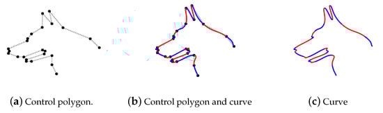
Figure 1. Open trigonometric Hermite interpolation curve. The restriction of the curve to the interval $[x_i,x_{i+1}],0\le i\le n-1,$ is shown (solid curve) with a red or blue color.

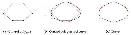
Figure 2. Closed trigonometric Hermite interpolation curve. The restriction of the curve to the interval $[x_i,x_{i+1}],0\le i\le n-1,$ is shown (solid curve) with a red or blue color.

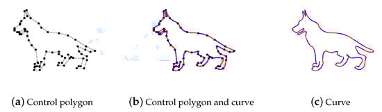
Figure 3. Closed trigonometric Hermite interpolation curve. The restriction of the curve to the interval $[x_i,x_{i+1}],0\le i\le n-1,$ is shown (solid curve) with a red or blue color.

4. TCB-Curves

In the previous section, we constructed open and closed trigonometric Hermite interpolation curves using the derivatives. In the present section, we are interested in another type of interpolation while using tcb, as described in details by Kochanek and Bartels (see [2]); it is a very powerful type of interpolation, its acronym is Tension, Continuity, Bias. These are the three characteristics that define the shape of the curve when the value of an interpolated parameter is determined over time. This type of interpolation produces a smooth curve between passing adjacent points, in the same way as the spline tool produces a smooth curve between the neighboring vertexes of the spline.

Each of these parameters has an important effect to better interpolate curves:

The tension parameter t controls how sharply the curve bends at a key position $P_i$, in some cases a large curve is desired, while, in other cases, it is preferred something more abrupt.

The continuity parameter c is used to avoid discontinuities in the direction and speed of motion, which are produced by linear interpolation.

The bias parameter b controls the direction of the path of a curve as it passes through a key position $P_i$.

In the following, we will apply a combination of the three parameters to open and closed Hermite interpolation curves and discuss the influence of each parameter on the interpolation curve.

More precisely, we are interested in the control values of type Kochanek–Bartels given by the vector:

$${[P_i,P_{i+1},D{D}_i,D{S}_{i+1}]}^T,$$

where, the destination derivative $D{D}_i$ and the source derivative $D{S}_i$ at $P_i$ are given, respectively, by:

$$\begin{array}{ccc}\hfill D{D}_i& =& \frac{(1-t)(1-c)(1+b)}{2}(P_i-P_{i-1})+\frac{(1-t)(1+c)(1-b)}{2}(P_{i+1}-P_i)\hfill \end{array}$$

and

$$\begin{array}{ccc}\hfill D{S}_i& =& \frac{(1-t)(1+c)(1+b)}{2}(P_i-P_{i-1})+\frac{(1-t)(1-c)(1-b)}{2}(P_{i+1}-P_i).\hfill \end{array}$$

Afterwards, we can define the trigonometric Kochanek-Bartels interpolation curve as

$$\begin{array}{ccc}\hfill C\left(x\right)& =& C_i\left(\frac{\pi }{2}\frac{x-x_i}{h}\right),x\in [x_i,x_{i+1}],\hfill \end{array}$$

where, for $u\in [0,\frac{\pi }{2}]$

$$\begin{array}{ccc}\hfill C_i\left(u\right)& =& P_i{\varphi }_0\left(u\right)+P_{i+1}{\varphi }_1\left(u\right)+\frac{2h}{\pi }D{D}_i{\varphi }_2\left(u\right)+\frac{2h}{\pi }D{S}_{i+1}{\varphi }_3\left(u\right).\hfill \end{array}$$

(9)

Examples

A trigonometric Hermite interpolation curve between two consecutive points $P_i$ and $P_{i+1}$ is based on these points’ position and the derivative associated at each point. The choice of the derivative with each point strongly affects the resulting trigonometric Hermite curve. We define the trigonometric Hermite curve on each segment $[x_i,x_{i+1}]$ using the two control points $P_i$ and $P_{i+1}$, and by specifying the tangent ($D{D}_i$ and $D{S}_i$) to the curve at each control point in terms of $(P_i-P_{i-1})$ and $(P_{i+1}-P_i)$ and with different values of t, c and b (see Figure 4, Figure 5, Figure 6 and Figure 7). The restriction of the trigonometric Hermite interpolation curve to the interval $[x_i,x_{i+1}],0\le i\le n-1,$ (see Figure 4 and Figure 6) is shown (solid curve) with a red or blue color.

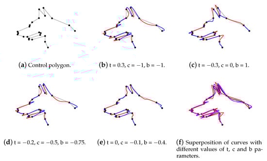
Figure 4. Trigonometric Hermite interpolation of open curves with clear effect of tension, continuity, and bias parameters.

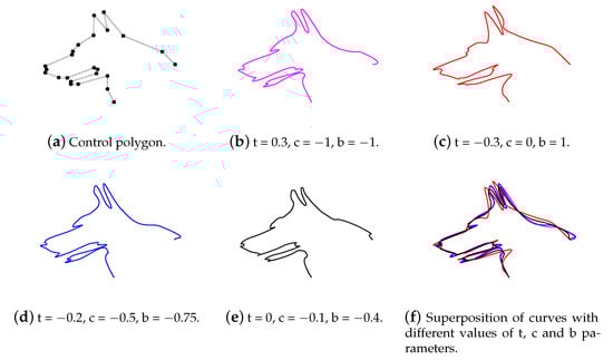
Figure 5. Effect of the combination of tension, continuity, and bias parameters on the interpolation of open curves.

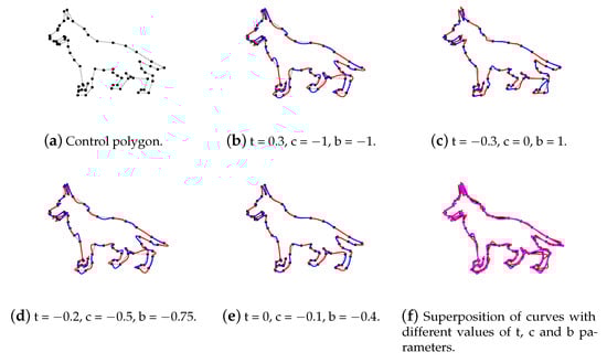
Figure 6. The effect of various parameter settings tcb on the interpolation of closed curves.

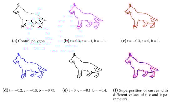
Figure 7. The effect of varying the tension, continuity and bias parameters on the closed curves.

5. ${\mathcal{C}}^1$ interpolation Hermite Surface

In this section, we present the natural extension of our trigonometric Hermite curve to the rectangular case. The reader is referred to [6,7,8,9,10,11] for similar works. Typically, the extension of a 1D Hermite interpolation curve to the tensor-product case is straightforward and it can be done as for the classical cubic case (see, e.g., [11]).

Let m and n be two positive integers, and consider $(m+1)\times (n+1)$ control point values $P_{i,j}$, and the first derivatives $D_{i,j}^u$, $D_{i,j}^v$ and $D_{i,j}^{u,v}$ corresponding to the rectangular grid points $(u_i,v_j)$, $i=0,\dots ,m,$ $j=0,\dots ,n$ (with $u_i=ih$, $v_j=jk$, $h=\frac{\pi }{2m}$ and $k=\frac{\pi }{2n}$). We can define the two-dimensionnel trigonometric Hermite interpolation, as follows:

Definition 1.

The ${(i,j)}^{th}$ bi-trigonometric Hermite partially Coons patch $S_{i,j}(u,v)$, assuming values $P_{i,j}$ and derivatives $D_{i,j}^u$, $D_{i,j}^v$ and $D_{i,j}^{u,v}$, corresponding to the four corners of the domain $[u_i,u_{i+1}]\times [v_j,v_{j+1}],$ can be defined by the matrix form: for $u\in [0,\frac{\pi }{2}]$, $v\in [0,\frac{\pi }{2}]$

$$\begin{array}{c}\hfill S_{i,j}(u,v)={\left[\begin{array}{c}{\varphi }_0\left(u\right)\\ {\varphi }_1\left(u\right)\\ {\varphi }_2\left(u\right)\\ {\varphi }_3\left(u\right)\end{array}\right]}^T\left[\begin{array}{cccc}{P}_{i,j}& P_{i,j+1}& \frac{2k}{\pi }{D}_{i,j}^v& \frac{2k}{\pi }{D}_{i,j+1}^v\\ P_{i+1,j}& P_{i+1,j+1}& \frac{2k}{\pi }{D}_{i+1,j}^v& \frac{2k}{\pi }{D}_{i+1,j+1}^v\\ \frac{2h}{\pi }{D}_{i,j}^u& \frac{2h}{\pi }{D}_{i,j+1}^u& \frac{4hk}{{\pi }^2}{D}_{i,j}^{u,v}& \frac{4hk}{{\pi }^2}{D}_{i,j+1}^{u,v}\\ \frac{2h}{\pi }{D}_{i+1,j}^u& \frac{2h}{\pi }{D}_{i+1,j+1}^u& \frac{4hk}{{\pi }^2}{D}_{i+1,j}^{u,v}& \frac{4hk}{{\pi }^2}{D}_{i+1,j+1}^{u,v}\end{array}\right]\left[\begin{array}{c}{\varphi }_0\left(v\right)\\ {\varphi }_1\left(v\right)\\ {\varphi }_2\left(v\right)\\ {\varphi }_3\left(v\right)\end{array}\right]\end{array}$$

Subsequently, the trigonometric Hermite interpolation surface is given by:

For $u\in [u_i,u_{i+1}],v\in [v_j,v_{j+1}],$

$$\begin{array}{c}\hfill S(u,v)=S_{i,j}(\frac{\pi }{2}\frac{u-u_i}{h},\frac{\pi }{2}\frac{v-v_i}{k}).\end{array}$$

(10)

The surface $S(u,v)$ has the interpolating property and it is ${\mathcal{C}}^1$-continuous. More precisely, we have the following lemma.

Lemma 2.

The ${(i,j)}^{th}$ bi-trigonometric Hermite partially Coons patch $S_{i,j}(u,v)$ verifies the following interpolating properties:

$$\begin{array}{c}\hfill \left\{\begin{array}{c}{S}_{i,j}(u_{i+p},v_{j+q})=P_{i+p,j+q},\hfill \\ \frac{\partial }{\partial u}{S}_{i,j}(u_{i+p},v_{j+q})=D_{i+p,j+q}^u,\hfill \\ \frac{\partial }{\partial v}{S}_{i,j}(u_{i+p},v_{j+q})=D_{i+p,j+q}^v,\hfill \\ \frac{{\partial }^2}{\partial u\partial v}{S}_{i,j}(u_{i+p},v_{j+q})=D_{i+p,j+q}^{u,v},\hfill \end{array}\right.\end{array}$$

with $p=0,1$ and $q=0,1.$

Proof. 

This follows immediately from the definition of $S_{i,j}(u,v)$. □

The surface $S(u,v)$ resulting frim the union of bi-trigonometric Hermite partially Coons patch $S_{i,j}(u,v)$ will have continuous first order derivatives and continuous crossed derivative. More precisely, we have the following result.

Proposition 1.

The surface $S(u,v)$ defined by (10) is ${\mathcal{C}}^1$-continuous.

Proof. 

It suffices to verify the following equations for all i and j.

$S_{i,j}(u_{i+1}^{+},v)=S_{i+1,j}(u_{i+1}^{-},v)=P_{i+1,j}{\varphi }_0(v)+P_{i+1,j+1}{\varphi }_1(v)+\frac{2k}{\pi }{D}_{i+1,j}^v{\varphi }_2(v)+\frac{2k}{\pi }{D}_{i+1,j+1}^v{\varphi }_3(v),$

$\frac{\partial }{\partial u}{S}_{i,j}(u_{i+1}^{+},v)=\frac{\partial }{\partial u}{S}_{i+1,j}(u_{i+1}^{-},v)=\frac{2h}{\pi }{D}_{i+1,j}^u{\varphi }_0(v)+\frac{2h}{\pi }{D}_{i+1,j+1}^u{\varphi }_1(v)+\frac{4hk}{{\pi }^2}{D}_{i+1,j}^{u,v}{\varphi }_2(v)+\frac{4hk}{{\pi }^2}{D}_{i+1,j+1}^{u,v}{\varphi }_3(v),$

$S_{i,j}(u,v_{j+1}^{+})=S_{i,j+1}(u,v_{j+1}^{-})=P_{i,j+1}{\varphi }_0(u)+P_{i+1,j+1}{\varphi }_1(u)+\frac{2h}{\pi }{D}_{i,j+1}^u{\varphi }_2(u)+\frac{2h}{\pi }{D}_{i+1,j+1}^u{\varphi }_3(u),$

$\frac{\partial }{\partial v}{S}_{i,j}(u,v_{j+1}^{+})=\frac{\partial }{\partial v}{S}_{i,j+1}(u,v_{j+1}^{-})=\frac{2k}{\pi }{D}_{i,j+1}^v{\varphi }_0(u)+\frac{2k}{\pi }{D}_{i+1,j+1}^v{\varphi }_1(u)+\frac{4hk}{{\pi }^2}{D}_{i,j+1}^{u,v}{\varphi }_2(u)+\frac{4hk}{{\pi }^2}{D}_{i+1,j+1}^{u,v}{\varphi }_3(u).$ □

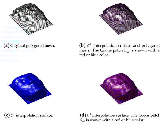
Example 1.

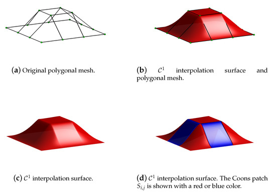
In Figure 8 and Figure 9, we present the original polygonal mesh, and the results that were obtained by ${\mathcal{C}}^1$ trigonometric Hermite interpolation surface defined previously by (10).

Figure 8. Original polygonal mesh (a) and the result obtained by ${\mathcal{C}}^1$ trigonometric Hermite interpolation surface derived here.

Figure 9. Original polygonal mesh of nefertiti (a) and the result obtained by ${\mathcal{C}}^1$ trigonometric Hermite interpolation surface (b–d).

6. Conclusions

New polynomial and trigonometric functions have been reported and are useful for constructing a new trigonometric Hermite interpolant. This Hermite interpolation led to building an interesting trigonometric Hermite basis having the same properties as Hermite polynomials’ classical basis. The tension, continuity, and bias parameters were combined and used as a potent type of interpolation. Surface construction using the studied trigonometric Hermite interpolation was explored. Several examples that were obtained by the ${\mathcal{C}}^1$ trigonometric Hermite interpolation surface were given to show the usefulness of this method.

References

- Catmull, E.; Rom, R. A class of local interpolating splines. In Computer Aided Geometric Design; Academic Press: Cambridge, MA, USA, 1974; pp. 317–326. [Google Scholar]
- Kochanek, D.H.U.; Bartels, R.H. Interpolating splines with local tension, continuity and Bias control. Comput. Graph. 1984, 18, 33–41. [Google Scholar] [CrossRef]
- Barrera, T.; Hast, A.; Bengtsson, E. Connected Minimal Acceleration Trigonometric Curves. Available online: https://ep.liu.se/ecp/016/001/ecp01601.pdf (accessed on 28 January 2021).
- Han, X. Piecewise trigonometric Hermite interpolation. Appl. Math. Comput. 2015, 268, 616–627. [Google Scholar] [CrossRef]
- Casciola, G.; Romani, L. Rational Interpolants with Tension Parameters. In Curve and Surface Design: Saint-Malo 2002; Lyche, T., Mazure, M., Schumaker, L.L., Eds.; Nashboro Press: Brentwood, UK, 2003. [Google Scholar]
- Zhang, C.; Wang, J. quartic spline surface interpolation. Sci. China Ser. F Inf. Sci. 2002, 45, 416–432. [Google Scholar]
- Duan, Q.; Li, S.; Bao, F.; Twizell, E.H. Hermite interpolation by piecewise rational surface. Appl. Math. Comput. 2008, 198, 59–72. [Google Scholar] [CrossRef]
- Fang, K.; Tan, J.; Zhu, G. - (-) Continuous Interpolation Spline Curve and Surface. J. Comput. Sci. Technol. 1998, 13, 238–245. [Google Scholar]
- Li, J. Cubic Trigonometric Hermite Parametric Curves and Surfaces with Shape Parameters. Int. J. Inf. Comput. Sci. 2012, 1, 8. [Google Scholar]
- Akima, H. A Method of Bivariate Interpolation and Smooth Surface Fitting Based on Local Procedures. Commun. ACM 1974, 17, 18–20. [Google Scholar] [CrossRef]
- Dodd, S.L.; McAllister, D.F.; Roulier, J.A. Shape-Preserving Spline Interpolation for Specifying Bivariate Functions on Grids. IEEE Comput. Graph. Appl. 1983, 3, 70–79. [Google Scholar] [CrossRef]
- Zhang, J. C-curves: An extension of cubic curves. Comput. Aided Geom. Des. 1996, 13, 199–217. [Google Scholar] [CrossRef]
- Li, J. A Class of Cubic Trigonometric Automatic Interpolation Curves and Surfaces with Parameters. Math. Comput. Appl. 2016, 21, 18. [Google Scholar] [CrossRef]
- Li, J.C.; Song, L.Z.; Liu, C.Z. The cubic trigonometric automatic interpolation spline. IEEE/CAA J. Autom. Sin. 2017, 5, 1136–1141. [Google Scholar] [CrossRef]
- BiBi, S.; Abbas, M.; Miura, K.T.; Misro, M.Y. Geometric Modeling of Novel Generalized Hybrid Trigonometric Bézier-Like Curve with Shape Parameters and Its Applications. Mathematics 2020, 8, 967. [Google Scholar] [CrossRef]
- Usman, M.; Abbas, M.; Miura, K.T. Some engineering applications of new trigonometric cubic Bézier-like curves to free-form complex curve modeling. J. Adv. Mech. Des. Syst. Manuf. 2020, 14, 1–15. [Google Scholar] [CrossRef]
Publisher’s Note: MDPI stays neutral with regard to jurisdictional claims in published maps and institutional affiliations. |
© 2021 by the authors. Licensee MDPI, Basel, Switzerland. This article is an open access article distributed under the terms and conditions of the Creative Commons Attribution (CC BY) license (http://creativecommons.org/licenses/by/4.0/).