Half-Space Relaxation Projection Method for Solving Multiple-Set Split Feasibility Problem

Abstract

In this paper, we study an iterative method for solving the multiple-set split feasibility problem: find a point in the intersection of a finite family of closed convex sets in one space such that its image under a linear transformation belongs to the intersection of another finite family of closed convex sets in the image space. In our result, we obtain a strongly convergent algorithm by relaxing the closed convex sets to half-spaces, using the projection onto those half-spaces and by introducing the extended form of selecting step sizes used in a relaxed CQ algorithm for solving the split feasibility problem. We also give several numerical examples for illustrating the efficiency and implementation of our algorithm in comparison with existing algorithms in the literature.

1. Introduction

1.1. Split Inverse Problem

Split Inverse Problem (SIP) is an archetypal model presented in ([1], Section 2), and it is stated as

$$\left\{\begin{array}{c}\mathrm{find}{x}^{\ast }\in X\mathrm{that} \mathrm{solves} \mathrm{IP}1\hfill \\ \mathrm{such} \mathrm{that}\hfill \\ y^{\ast }=A{x}^{\ast }\in Y\mathrm{and} \mathrm{solves} \mathrm{IP}2\hfill \end{array}\right.$$

where A is a bounded linear operator from a space X to another space Y, and IP1 and IP2 are two inverse problems installed in X and Y, respectively. Real-world inverse problems can be cast into this framework by making different choices of the spaces X and Y (including the case $X=Y$), and by choosing appropriate inverse problems for IP1 and IP2. For example, image restoration, computer tomograph and intensity-modulated radiation therapy (IMRT) treatment planning generate functions that can be transformed to have an SIP model; see in [2,3,4,5]. The split feasibility problem [6] and multiple-set split feasibility problem [7] are the first instances of the SIP, where the two problems IP1 and IP2 are of the Convex Feasibility Problem (CFP) type [8]. In the SIP framework, many authors studied cases for which IP1 and IP2 are convex feasibility problems, minimization problems, equilibrium problems, fixed point problems, null point problems and so on; see, for example [2,3,5,9,10,11,12,13,14,15,16,17,18,19,20].

1.2. Split Feasibility Problem and Multiple-Set Split Feasibility Problem

Let H be a real Hilbert space and let $T:H\to H$ be an operator. We say that T is $\rho$-strongly quasi-nonexpansive, where $\rho \ge 0$, if Fix$T=\{x\in H:Tx=x\}\ne Ø$ and

$${\parallel Tx-p\parallel }^2\le {\parallel x-p\parallel }^2-\rho {\parallel Tx-p\parallel }^2,\forall (x,p)\in H\times \mathrm{Fix}T.$$

(1)

If $\rho =0$ in (1), then T is called a quasi-nonexpansive operator. If $\rho >0$ in (1), then we say that T is strongly quasi-nonexpansive. Obviously, a nonexpansive operator having a fixed point is quasi-nonexpansive. If T is quasi-nonexpansive, then FixT is closed and convex. For $\nu \ge 0$ denote by $T_{\nu }:=(1-\nu )I+\nu T$, the $\nu$-relaxation of T, where I is the identity operator and $\nu$ is called relaxation parameter. If T is quasi-nonexpansive, then usually one applies a relaxation parameter $\nu \in [0,1]$.

Let $H_1$ and $H_2$ be real Hilbert spaces and let $A:H_1\to H_2$ be a bounded linear operator. Given a nonempty closed convex subsets $\{C_1,\dots ,C_N\}$ and $\{Q_1,\dots ,Q_M\}$ of $H_1$ and $H_2$, respectively. The Multiple-Set Split Feasibility Problem (MSSFP), which was introduced by Censor et al. [7], is formulated as finding a point

$$\overline{x}\in {\displaystyle \bigcap _{i=1}^N}{C}_i \mathrm{such} \mathrm{that} A\overline{x}\in {\displaystyle \bigcap _{j=1}^M}{Q}_j.$$

(2)

Denote by $\mathsf{\Omega }$ the set of solutions for (2). The MSSFP (2) with $N=M=1$ is known as the Split Feasibility Problem (SFP), which is formulated as finding a point

$$\overline{x}\in C \mathrm{such} \mathrm{that} A\overline{x}\in Q,$$

(3)

where C and Q are nonempty closed convex subsets of real Hilbert spaces $H_1$ and $H_2$, respectively. The SFP was first introduced in 1994 by Censor and Elfving [6] for modeling inverse problems in finite-dimensional Hilbert spaces for modeling inverse problems that arise from phase retrievals and in medical image reconstruction. SFP plays an important role in the study of signal processing, image reconstruction, intensity-modulated radiation, therapy, etc. [2,3,5,11]. Several iterative algorithms were presented to solve the SFP and MSSFP provided the solution exists; see, for example, in [3,6,21,22,23,24,25,26,27,28,29,30,31,32]. The algorithm proposed by Censor and Elfving [6] for solving the SFP involves the computation of the inverse of A per each iteration assuming the existence of the inverse of A, a fact that makes the algorithm nonapplicable in practice. Most methods employ the Landweber operators, see the definition and its property in [33]. In general, all of these methods produce sequences that converge weakly to a solution. Byrne [3] proposed the following iteration for solving the SFP, and called it the CQ-algorithm or the projected Landweber method:

$$x_{n+1}=P_C{V}_{\nu }\left(x_n\right),$$

(4)

where $x_1\in H_1$ is arbitrary, $V_{\nu }$ is a $\nu$-relaxation of the Landweber operator V (corresponding to $P_Q$), i.e.,

$$V=I-\frac{1}{{\parallel A\parallel }^2}{A}^{\ast }(I-P_Q)A,$$

where $\nu \in (0,2)$, $A^{\ast }$ denotes the adjoint of A, and ${\parallel A\parallel }^2$ is the spectral norm of $A{A}^{\ast }$. It is well known that the CQ algorithm (4) does not necessarily converge strongly to the solution of SFP in the infinite-dimensional Hilbert space. An important advantage of the $CQ$ algorithm by Byrne [3,21] is that computation of the inverse of A (matrix inverses) is not necessary. The Landweber operator is used for a more general type of problem called the split common fixed point problem of quasi-nonexpansive operators (see, for example, [10,34,35]), but the implementation of the Landweber-type algorithm generated requires prior knowledge of the operator norm. However, the operator norm is a global invariant and is often difficult to estimate; see, for example, the Theorem of Hendrickx and Olshevsky in [36]. To overcome this difficulty, Lopez et al. [2] introduced a new way of selecting the step sizes for solving the SFP (3) such that the information of the operator norm is not necessary. To be precise, Lopez et al. [2] proposed

$$x_{n+1}=P_C(I-{\gamma }_n{A}^{\ast }(I-P_Q)A)x_n,$$

where ${\gamma }_n=\frac{{\rho }_{n}f\left(x_n\right)}{\parallel \nabla f\left(x_n\right){\parallel }^2},\forall n\ge 1$, ${\rho }_n\in (0,4)$, $f\left(x_n\right)=\frac{1}{2}{\parallel (I-P_Q)A{x}_n\parallel }^2$ and $\nabla f\left(x_n\right)=A^{\ast }(I-P_Q)A{x}_n$. In addition, the computation of the projection on a closed convex set is not easy. In order to overcome this drawback, Yang [37] considered SFPs in which the involved sets C and Q are given as sub-level sets of convex functions, i.e.,

$$C=\{x\in H_1:c\left(x\right)\le 0\} \mathrm{and} Q=\{y\in H_2:q\left(y\right)\le 0\},$$

(5)

where $c:H_1\to \mathbb{R}$ and $q:H_2\to \mathbb{R}$ are convex and subdifferentiable functions on $H_1$ and $H_2$, respectively, and that $\partial c$ and $\partial q$ are bounded operators (i.e., bounded on bounded sets). It is known that every convex function defined on a finite-dimensional Hilbert space is subdifferentiable and its subdifferential operator is a bounded operator (see [38]). In this situation, the efficiency of the $CQ$ method is extremely affected because, in general, the computation of projections onto such subsets is still very difficult. Motivated by Fukushima’s relaxed projection method in [39], Yang [37] suggested calculating the projection onto a half-space containing the original subset instead of the latter set itself. More precisely, Yang introduced a relaxed $CQ$ algorithm using a half-space relaxation projection method for solving SFP. The proposed algorithm by Yang is given as follows:

$$x_{n+1}=P_{C_n}(x_n-\gamma f_n\left(x_n\right)),$$

where $f_n=A^{\ast }(I-P_{Q_n})A$, for each $n\in \mathbb{N}$ the set $C_n$ is given by

$$C_n=\{x\in H_1:c\left(x_n\right)\le ⟨{\xi }_n,x_n-x⟩\},$$

(6)

where ${\xi }_n\in \partial c\left(x_n\right)$, and the set $Q_n$ is given by

$$Q_n=\{y\in H_2:q\left(A{x}_n\right)\le ⟨{\epsilon }_n,A{x}_n-y⟩\},$$

(7)

where ${\epsilon }_n\in \partial q\left(A{x}_n\right)$. Obviously, $C_n$ and $Q_n$ are half-spaces and $C\subset C_n$ and $Q\subset Q_n$ for every $n\ge 1$. More important, since the projections onto $C_n$ and $Q_n$ have the closed form, the relaxed $CQ$ algorithm is now easily implemented. The specific form of the metric projections onto $C_n$ and $Q_n$ can be found in [38,40,41].

For solving the MSSFP (2), many methods have been developed; see, for example, in [7,26,42,43,44,45,46,47,48,49] and references therein. We aim to propose a strongly convergent algorithm with high efficiency that is easy to implement in solving the MSSFP. Motivated by Yang [37], we are interested in solving the MSSFP (2) in which the involved sets $C_i$ ($i\in \{1,\dots ,N\}$) and $Q_j$ ($j\in \{1,\dots ,M\}$) are given as sub-level sets of convex functions, i.e.,

$$C_i=\{x\in H_1:c_i\left(x\right)\le 0\}\mathrm{and} Q_j=\{y\in H_2:q_j\left(y\right)\le 0\},$$

(8)

where $c_i:H_1\to \mathbb{R}$ and $q_j:H_2\to \mathbb{R}$ are convex functions for all $i\in \{1,\dots ,N\}$, $j\in \{1,\dots ,M\}$. We assume that each $c_i$ and $q_j$ are subdifferentiable on $H_1$ and $H_2$, respectively, and that $\partial c_i$ and $\partial q_j$ are bounded operators (i.e., bounded on bounded sets). In what follows, we define $N+M$ half-spaces at point $x_n$ by

$$C_{i,n}=\{x\in H_1:c_i\left(x_n\right)\le ⟨{\xi }_{i,n},x_n-x⟩\},$$

(9)

where ${\xi }_{i,n}\in \partial c_i\left(x_n\right)$, and

$$Q_{j,n}=\{y\in H_2:q_j\left(A{x}_n\right)\le ⟨{\epsilon }_{j,n},A{x}_n-y⟩\},$$

(10)

where ${\epsilon }_{j,n}\in \partial q_j\left(A{x}_n\right)$.

The paper contributes to developing the algorithm for the MSSFP in the direction of half-space relaxation (assuming $C_i$ and $Q_j$ are given as a sub-level sets of convex functions (8)) and parallel computation of projection onto half-spaces (9) and (10) without prior knowledge of the operator norm.

This paper is organized in the following way. In Section 2, we recall some basic and useful facts that will be used in the proof of our results. In Section 3, we introduce the extended form of the way of selecting step sizes used in the relaxed CQ algorithm for solving the SFP by [37] and Lopez et al. [2] to work for the MSSFP framework, and we analyze the strong convergence of our proposed algorithm. In Section 4, we give some numerical examples to discuss the performance of the proposed algorithm. Finally, we give some conclusions.

2. Preliminary

In this section, in order to prove our result, we recall some basic notions and useful results in a real Hilbert space H. The symbols $"\rightharpoonup "$ and $"\to "$ denote weak and strong convergence, respectively.

Let C be a nonempty closed convex subset of H. The metric projection on C is a mapping $P_C:H\to C$ defined by

$$P_C\left(x\right)=argmin\{\parallel y-x\parallel :y\in C\},x\in H.$$

Lemma 1. 

[50] Let C be a closed convex subset of H. Given $x\in H$ and a point $z\in C$, then $z=P_C\left(x\right)$ if and only if

$$⟨x-z,y-z⟩\le 0,\forall y\in C.$$

The mapping $T:H\to H$ is firmly nonexpansive if

$${\parallel Tx-Ty\parallel }^2\le {\parallel x-y\parallel }^2{-\left|\right|(I-T)x-(I-T)y\parallel }^2,\forall x,y\in H,$$

which is equivalent to

$${\parallel Tx-Ty\parallel }^2\le ⟨Tx-Ty,x-y⟩,\forall x,y\in H.$$

If T is firmly nonexpansive, $I-T$ is also firmly nonexpansive. The metric projection $P_C$ on a closed convex subset C of H is firmly nonexpansive.

Definition 1. 

The subdifferential of a convex function $f:H\to \mathbb{R}$ at $x\in H$, denoted by $\partial f\left(x\right)$, is defined by

$$\partial f\left(x\right)=\{\xi \in H:f(z)\ge f(x)+⟨\xi ,z-x⟩,\forall z\in H\}.$$

If $\partial f\left(x\right)\ne Ø$, f is said to be subdifferentiable at x. If the function f is continuously differentiable then $\partial f\left(x\right)=\{\nabla f(x\left)\right\}$, this is the gradient of f.

Definition 2. 

The function $f:H\to \mathbb{R}$ is called weakly lower semi-continuous at $x_0$ if the sequence $\left\{x_n\right\}$ weakly converges to $x_0$ implies

$$\underset{n\to \infty }{lim\; inf}f\left(x_n\right)\ge f\left(x_0\right).$$

A function that is weakly lower semi-continuous at each point of H is called weakly lower semi-continuous on H.

Lemma 2. 

[3,51] Let $H_1$ and $H_2$ be real Hilbert spaces and $f:H_1\to \mathbb{R}$ is given by $f\left(x\right)=\frac{1}{2}{\parallel (I-P_Q)Ax\parallel }^2$ where Q is closed convex subset of $H_2$ and $A:H_1\to H_2$ be a bounded linear operator. Then

(i) 

The function f is convex and weakly lower semi-continuous on $H_1$;

(ii) 

$\nabla f\left(x\right)=A^{\ast }(I-P_Q)Ax$ for $x\in H_1$;

(iii) 

$\nabla f$ is ${\parallel A\parallel }^2$-Lipschitz, i.e., $\parallel \nabla f\left(x\right)-\nabla f\left(y\right)\parallel \le {\parallel A\parallel }^2\parallel x-y\parallel ,\forall x,y\in H_1.$

Lemma 3. 

[27,52] Let C and Q be closed convex subsets of real Hilbert spaces $H_1$ and $H_2$, respectively, and $f:H_1\to \mathbb{R}$ is given by $f\left(x\right)=\frac{1}{2}{\parallel (I-P_Q)Ax\parallel }^2$, where $A:H_1\to H_2$ be a bounded linear operator. Then for $\lambda >0$ and $\overline{x}\in H_1$ the following statements are equivalent.

(i) 

The point $\overline{x}$ solves the SFP (3), i.e., $\overline{x}\in \{x\in C:Ax\in Q\}$;

(ii) 

The point $\overline{x}$ is the fixed point of the mapping $P_C(I-\lambda \nabla f)$, i.e.,

$$P_C(\overline{x}-\lambda \nabla f\left(\overline{x}\right))=\overline{x}.$$

Lemma 4. 

[53] Let H be a real Hilbert space. Then, for all $x,y\in H$ and $\alpha \in [0,1]$, we have

(i) 

${\parallel \alpha x+(1-\alpha )y\parallel }^2={\alpha \parallel x\parallel }^2+{(1-\alpha )\parallel y\parallel }^2-\alpha (1-\alpha ){\parallel x-y\parallel }^2;$

(ii) 

${\parallel x+y\parallel }^2={\parallel x\parallel }^2+{\parallel y\parallel }^2+2⟨x,y⟩;$

(iii) 

${\parallel x+y\parallel }^2\le {\parallel x\parallel }^2+2⟨y,x+y⟩.$

Lemma 5. 

[54] Let $\left\{a_n\right\}$ be the sequence of nonnegative numbers such that

$$a_{n+1}\le (1-{\alpha }_n)a_n+{\alpha }_n{\delta }_n,$$

where $\left\{{\delta }_n\right\}$ is a sequence of real numbers bounded from above and $0\le {\alpha }_n\le 1$ and ${\displaystyle \sum _{n=1}^{\infty }}{\alpha }_n=\infty$. Then it holds that

$$\underset{n\to \infty }{lim\; sup}{\alpha }_n\le \underset{n\to \infty }{lim\; sup}{\delta }_n.$$

3. Half-Space Relaxation Projection Algorithm

In this section, we propose an iterative algorithm to solve the MSSFP (2). To make our algorithm more efficient and the implementation of the algorithm more easy, we assume that the convex sets $C_i$ and $Q_j$ are given in the form of (8) and we use projections onto half-spaces $C_{i,n}$ and $Q_{j,n}$ defined in (9) and (10), respectively, instead of onto $C_i$ and $Q_j$, just as the relaxed or inexact methods in [5,37,39,55]. Moreover, in order to remove the requirement of the estimated value of the operator norm and solve the MSSFP when finding the operator norm is not easy, we now introduce a new way of selecting the step sizes for solving the MSSFP (2) given as follows for $x\in H_1$, and $C_{i,n}$ and $Q_{j,n}$ are half-spaces defined in (9) and (10).

(i) 

For each $i\in \{1,\dots ,N\}$ and $n\ge 1$, define

$$g_{i,n}\left(x\right)=\frac{1}{2}{\parallel (I-P_{C_{i,n}})x\parallel }^2\mathrm{and} \mathrm{so}\nabla g_{i,n}\left(x\right)=(I-P_{C_{i,n}})x.$$

(ii) 

$g_n\left(x\right)$ and $\nabla g_n\left(x\right)$ are defined as $g_n\left(x\right)=g_{i_{n_x},n}\left(x\right)$ and so $\nabla g_n\left(x\right)=\nabla g_{i_{n_x},n}\left(x\right)$ where $i_{n_x}\in \{1,\dots ,N\}$ such that for each $n\ge 1$,

$$i_{n_x}\in argmax\{g_{i,n}\left(x\right):i\in \{1,\dots ,N\}\}.$$

(iii) 

For each $j\in \{1,\dots ,M\}$ and $n\ge 1$, define

$$f_{j,n}\left(x\right)=\frac{1}{2}{\parallel (I-P_{Q_{j,n}})Ax\parallel }^2\mathrm{and} \nabla f_{j,n}\left(x\right)=A^{\ast }(I-P_{Q_{j,n}})Ax.$$

From Aubin [51], $g_{i,n}$ and $f_{j,n}$ are convex, weakly lower semi-continuous and differentiable for each $i\in \{1,\dots ,N\}$ and $j\in \{1,\dots ,M\}$. Now, using $\nabla g_{i,n}$, $g_{i,n}$, $g_n$, $\nabla g_n$, $f_{j,n}$ and $\nabla f_{j,n}$ given in (i)–(iii) above, and assuming that the solution set $\mathsf{\Omega }$ of the MSSFP (2) is nonempty, we propose and analyze the strong convergence of our algorithm, called the Half-Space Relaxation Projection Algorithm.

Note that, the iterative scheme in Algorithm 1 (HSRPA) is established in away that $\nabla g_n\left(z_n\right)$ and $\nabla f_{j,n}\left(z_n\right)$ are computed, i.e., the projections $P_{C_{i,n}}$ and $P_{Q_{j,n}}$ are computed, in parallel setting under simple assumptions on step sizes.

Algorithm 1: Half-Space Relaxation Projection Algorithm (HSRPA).

Initialization: Choose u, $x_1\in H_1$. Let the positive real constants ${\lambda }_1$, ${\lambda }_2$ and ${\delta }_j$ ($j=1,\dots ,M$),   and the real sequences $\left\{{\alpha }_n\right\}$, $\left\{{\beta }_n\right\}$ and $\left\{{\rho }_n\right\}$ satisfy the following conditions:   (C1)  ${\lambda }_1,{\lambda }_2\in (0,1)$ and ${\lambda }_1+{\lambda }_2=1$.   (C2)  $0<{\delta }_j<1$ for all $j\in \{1,\dots ,M\}$, and ${\displaystyle \sum _{j=1}^M}{\delta }_j=1$.   (C3)  $0<{\alpha }_n<1$, $\underset{n\to \infty }{lim}{\alpha }_n=0$ and ${\displaystyle \sum _{n=1}^{\infty }}{\alpha }_n=\infty$.   (C4)  $0<a\le {\beta }_n\le b<1$ for all $n\in \mathbb{N}$.   (C5)  $0<\lambda {\rho }_n<4\overline{\lambda }$ and $\underset{n\to \infty }{lim\; inf}{\rho }_n(4\overline{\lambda }-\lambda {\rho }_n)>0$, where $\lambda =max\{{\lambda }_1,{\lambda }_2\}$ and   $\overline{\lambda }=min\{{\lambda }_1,{\lambda }_2\}$.  Iterative Step: Proceed with the following computations: $$\left\{\begin{array}{c}{z}_n=(1-{\alpha }_n)x_n+{\alpha }_{n}u,\hfill \\ y_n=z_n-{\displaystyle \sum _{j=1}^M}{\delta }_j{\tau }_{j,n}({\lambda }_1\nabla g_n\left(z_n\right)+{\lambda }_2\nabla f_{j,n}\left(z_n\right)),\hfill \\ x_{n+1}=(1-{\beta }_n)z_n+{\beta }_n{y}_n\hfill \end{array}\right.$$  where $${\tau }_{j,n}={\rho }_n\frac{f_{j,n}\left(z_n\right)+g_n\left(z_n\right)}{d_j\left(z_n\right)},$$  for $$d_j\left(z_n\right)=\left\{\begin{array}{c}1,\mathrm{if}\parallel \nabla g_n\left(z_n\right){\parallel }^2+{\parallel \nabla f_{j,n}\left(z_n\right)\parallel }^2=0\hfill \\ \parallel \nabla g_n\left(z_n\right){\parallel }^2+{\parallel \nabla f_{j,n}\left(z_n\right)\parallel }^2,\mathrm{otherwise}.\hfill \end{array}\right..$$

Lemma 6. 

If $\{j\in \{1,\dots ,M\}:\parallel \nabla g_n\left(z_n\right){\parallel }^2+\parallel \nabla f_{j,n}\left(z_n\right){\parallel }^2\ne 0\}=Ø$ at some iterate n in HSRPA, then $z_n$ is the solution of MSSFP (2).

Proof. 

$\{j\in \{1,\dots ,M\}:\parallel \nabla g_n\left(z_n\right){\parallel }^2+\parallel \nabla f_{j,n}\left(z_n\right){\parallel }^2\ne 0\}=Ø$ implies

$$\begin{array}{c}\parallel \nabla g_n\left(z_n\right){\parallel }^2+{\parallel \nabla f_{j,n}\left(z_n\right)\parallel }^2=0,\forall j\in \{1,\dots ,M\},\hfill \\ \iff \parallel \nabla g_n\left(z_n\right)\parallel =0=\parallel \nabla f_{j,n}\left(z_n\right)\parallel ,\forall j\in \{1,\dots ,M\},\hfill \\ \iff \parallel \nabla g_{i,n}\left(z_n\right)\parallel =0=\parallel \nabla f_{j,n}\left(z_n\right)\parallel ,\forall i\in \{1,\dots ,N\},\forall j\in \{1,\dots ,M\},\hfill \\ \iff (I-P_{C_{i,n}})\left(z_n\right)=0=A^{\ast }(I-P_{Q_{j,n}})A\left(z_n\right),\forall i\in \{1,\dots ,N\},\forall j\in \{1,\dots ,M\}.\hfill \end{array}$$

Thus, one can get $P_{C_{i,n}}(z_n-\lambda \nabla f_{j,n}\left(z_n\right))=z_n$ for all $i\in \{1,\dots ,N\}$ and $j\in \{1,\dots ,M\}$. Since $C_i\subset C_{i,n}$, we get $z_n\in C_{i,n}$ for all $i\in \{1,\dots ,N\}$. Combined with the fixed point relation Lemma 3 (ii), we also get that $A{z}_n\in Q_{j,n}$ for all $j\in \{1,\dots ,M\}$. Following the representations of the sets $C_{i,n}$ and $Q_{j,n}$ in (9) and (10) we obtain that $c_i\left(z_n\right)\le 0$ for all $i\in \{1,\dots ,N\}$ and $q_j\left(A{z}_n\right)\le 0$ for all $i\in \{1,\dots ,N\}$, and this implies that $z_n\in C_i$ for all $i\in \{1,\dots ,N\}$ and $A{z}_n\in Q_j$ for all $j\in \{1,\dots ,M\}$, which completes the proof. ☐

By Lemma 6, we can conclude that the HSRPA terminates at some iterate n when $\{j\in \{1,\dots ,M\}:\parallel \nabla g_n\left(z_n\right){\parallel }^2+\parallel \nabla f_{j,n}\left(z_n\right){\parallel }^2\ne 0\}=Ø$. Otherwise, if the HSRPA does not stop, then we have the following strong convergence theorem for the approximation of the solution of the problem of MSSFP (2).

Theorem 1. 

The sequence $\left\{x_n\right\}$ generated by HSRPA converges strongly to the solution point $\overline{x}$ of MSSFP (2) ($x_n\to \overline{x}\in \mathsf{\Omega }$) where $\overline{x}=P_{\mathsf{\Omega }}u$.

Proof. 

Let $\overline{x}\in \mathsf{\Omega }$. Since $I-P_{C_{i,n}}$ and $I-P_{Q_{j,n}}$ are firmly nonexpansive, and since $\overline{x}$ verifies (2), we have for all $x\in H_1$

$$\begin{array}{ccc}⟨\nabla g_{i,n}\left(x\right),x-\overline{x}⟩\hfill & =\hfill & ⟨(I-P_{C_{i,n}})x,x-\overline{x}⟩\hfill \\ & \ge \hfill & \parallel (I-P_{C_{i,n}}){x\parallel }^2=2g_{i,n}\left(x\right),\hfill \end{array}$$

(11)

and

$$\begin{array}{ccc}⟨\nabla f_{j,n}\left(x\right),x-\overline{x}⟩\hfill & =\hfill & ⟨A^{\ast }(I-P_{Q_{j,n}})Ax,x-\overline{x}⟩\hfill \\ & =\hfill & ⟨(I-P_{Q_{j,n}})Ax,Ax-A\overline{x}⟩\hfill \\ & \ge \hfill & \parallel (I-P_{Q_{j,n}}){Ax\parallel }^2=2f_{j,n}\left(x\right).\hfill \end{array}$$

(12)

Using definition of $y_n$ and Lemma 4$\left(ii\right)$, we have

$$\begin{array}{cc}\parallel y_n-\overline{x}{\parallel }^2\hfill & =\parallel z_n-{\displaystyle \sum _{j=1}^M}{\delta }_j{\tau }_{j,n}({\lambda }_1\nabla g_n\left(z_n\right)+{\lambda }_2\nabla f_{j,n}\left(z_n\right))-\overline{x}{\parallel }^2\hfill \\ & \le \parallel z_n-\overline{x}{\parallel }^2+\parallel {\displaystyle \sum _{j=1}^M}{\delta }_j{\tau }_{j,n}({\lambda }_1\nabla g_n\left(z_n\right)+{\lambda }_2\nabla f_{j,n}\left(z_n\right)){\parallel }^2\hfill \\ & -2⟨{\displaystyle \sum _{j=1}^M}{\delta }_j{\tau }_{j,n}({\lambda }_1\nabla g_n\left(z_n\right)+{\lambda }_2\nabla f_{j,n}\left(z_n\right)),z_n-\widehat{x}⟩.\hfill \end{array}$$

(13)

Using convexity of ${\parallel .\parallel }^2$, we have

$$\begin{array}{c}\parallel {\displaystyle \sum _{j=1}^M}{\delta }_j{\tau }_{j,n}({\lambda }_1\nabla g_n\left(z_n\right)+{\lambda }_2\nabla f_{j,n}\left(z_n\right)){\parallel }^2\hfill \\ \hspace{1em}\le {\displaystyle \sum _{j=1}^M}{\delta }_j{\left({\tau }_{j,n}\right)}^2\parallel {\lambda }_1\nabla g_n\left(z_n\right)+{\lambda }_2\nabla f_{j,n}\left(z_n\right){\parallel }^2\hfill \\ \hspace{1em}\le {\displaystyle \sum _{j=1}^M}{\delta }_j{\left({\tau }_{j,n}\right)}^2({\lambda }_1\parallel \nabla g_n\left(z_n\right){\parallel }^2+{\lambda }_2\parallel \nabla f_{j,n}\left(z_n\right){\parallel }^2)\hfill \\ \hspace{1em}\le {\displaystyle \sum _{j=1}^M}\left\{\lambda {\delta }_j{\left({\rho }_n\frac{f_{j,n}\left(z_n\right)+g_n\left(z_n\right)}{d_j\left(z_n\right)}\right)}^2(\parallel \nabla g_n\left(z_n\right){\parallel }^2+\parallel \nabla f_{j,n}\left(z_n\right){\parallel }^2)\right\}\hfill \\ \hspace{1em}\le {\displaystyle \sum _{j=1}^M}\left\{\lambda {\delta }_j{\left({\rho }_n\frac{f_{j,n}\left(z_n\right)+g_n\left(z_n\right)}{d_j\left(z_n\right)}\right)}^2{d}_j\left(z_n\right)\right\}\hfill \\ \hspace{1em}=\lambda {\rho }_n^2{\displaystyle \sum _{j=1}^M}\left\{{\delta }_j\frac{{(f_{j,n}\left(z_n\right)+g_n\left(z_n\right))}^2}{d_j\left(z_n\right)}\right\}.\hfill \end{array}$$

(14)

From (11) and (12), we have

$$\begin{array}{c}⟨{\displaystyle \sum _{j=1}^M}{\delta }_j{\tau }_{j,n}({\lambda }_1\nabla g_n\left(z_n\right)+{\lambda }_2\nabla f_{j,n}\left(z_n\right)),z_n-\widehat{x}⟩\hfill \\ \hspace{1em}={\displaystyle \sum _{j=1}^M}{\delta }_j{\tau }_{j,n}⟨({\lambda }_1\nabla g_n\left(z_n\right)+{\lambda }_2\nabla f_{j,n}\left(z_n\right),z_n-\widehat{x}⟩\hfill \\ \hspace{1em}={\displaystyle \sum _{j=1}^M}{\delta }_j{\tau }_{j,n}({\lambda }_1⟨\nabla g_n\left(z_n\right),z_n-\widehat{x}⟩+{\lambda }_2⟨\nabla f_{j,n}\left(z_n\right),z_n-\widehat{x}⟩)\hfill \\ \hspace{1em}\ge {\displaystyle \sum _{j=1}^M}{\delta }_j{\tau }_{j,n}(2{\lambda }_1{g}_n\left(z_n\right)+2{\lambda }_2{f}_{j,n}\left(z_n\right))\hfill \\ \hspace{1em}={\displaystyle \sum _{j=1}^M}\left\{{\delta }_j{\rho }_n\frac{f_{j,n}\left(z_n\right)+g_n\left(z_n\right)}{d_j\left(z_n\right)}(2{\lambda }_1{g}_n\left(z_n\right)+2{\lambda }_2{f}_{j,n}\left(z_n\right))\right\}\hfill \\ \hspace{1em}\ge 2\overline{\lambda }{\rho }_n{\displaystyle \sum _{j=1}^M}\left\{{\delta }_j\frac{{(f_{j,n}\left(z_n\right)+g_n\left(z_n\right))}^2}{d_j\left(z_n\right)}\right\}.\hfill \end{array}$$

(15)

In view of (13), (14) and (15), we have

$$\begin{array}{ccc}\parallel y_n-\overline{x}{\parallel }^2\hfill & \le \hfill & \parallel z_n-\overline{x}{\parallel }^2+\lambda {\rho }_n^2{\displaystyle \sum _{j=1}^M}\left\{{\delta }_j\frac{{(f_{j,n}\left(z_n\right)+g_n\left(z_n\right))}^2}{d_j\left(z_n\right)}\right\}\hfill \\ \hfill & & -4\overline{\lambda }{\rho }_n{\displaystyle \sum _{j=1}^M}\left\{{\delta }_j\frac{{(f_{j,n}\left(z_n\right)+g_n\left(z_n\right))}^2}{d_j\left(z_n\right)}\right\}\hfill \\ & =\hfill & \parallel z_n-\overline{x}{\parallel }^2+{\rho }_n(\lambda {\rho }_n-4\overline{\lambda }){\displaystyle \sum _{j=1}^M}\left\{{\delta }_j\frac{{(f_{j,n}\left(z_n\right)+g_n\left(z_n\right))}^2}{d_j\left(z_n\right)}\right\}.\hfill \end{array}$$

(16)

From (16) and (C5), we have

$$\parallel y_n-\overline{x}\parallel \le \parallel z_n-\overline{x}\parallel .$$

(17)

Using (17), Lemma 4 $\left(i\right)$ and the definition of $x_{n+1}$, we get

$$\begin{array}{ccc}\parallel x_{n+1}-\overline{x}{\parallel }^2\hfill & =\hfill & \parallel (1-{\beta }_n)z_n+{\beta }_n{y}_n-\overline{x}{\parallel }^2\hfill \\ & =\hfill & \parallel (1-{\beta }_n)(z_n-\overline{x})+{\beta }_n(y_n-\overline{x}){\parallel }^2\hfill \\ & =\hfill & (1-{\beta }_n)\parallel z_n-\overline{x}{\parallel }^2+{\beta }_n\parallel y_n-\overline{x}{\parallel }^2-{\beta }_n(1-{\beta }_n){\parallel z_n-y_n\parallel }^2\hfill \\ & \le \hfill & \parallel z_n-\overline{x}{\parallel }^2-{\beta }_n(1-{\beta }_n){\parallel z_n-y_n\parallel }^2.\hfill \end{array}$$

(18)

From (18) and the definition of $z_n$, we get

$$\begin{array}{cc}\parallel x_{n+1}-\overline{x}\parallel \le \parallel z_n-\overline{x}\parallel \hfill & =(1-{\alpha }_n)\parallel x_n-\overline{x}\parallel +{\alpha }_n\parallel u-\overline{x}\parallel \hfill \\ & \le max\{\parallel x_n-\overline{x}\parallel ,\parallel u-\overline{x}\parallel \}\hfill \\ & \hspace{1em}⋮\hfill \\ & \le max\{\parallel x_1-\overline{x}\parallel ,\parallel u-\overline{x}\parallel \},\hfill \end{array}$$

which shows that $\left\{x_n\right\}$ is bounded. Consequently, $\left\{z_n\right\}$, $\left\{A{z}_n\right\}$ and $\left\{y_n\right\}$ are all bounded.

Now,

$$\begin{array}{c}\frac{1}{{\beta }_n}(x_{n+1}-z_n)=\frac{1}{{\beta }_n}\left((1-{\beta }_n)z_n+{\beta }_n{y}_n-z_n\right)=y_n-z_n,\hfill \end{array}$$

(19)

and

$$\begin{array}{c}\parallel y_n-z_n{\parallel }^2=\frac{1}{{\beta }_n^2}{\parallel x_{n+1}-z_n\parallel }^2=\frac{{\alpha }_n}{{\beta }_n}\left(\frac{\parallel x_{n+1}-z_n{\parallel }^2}{{\alpha }_n{\beta }_n}\right).\hfill \end{array}$$

(20)

Using (18) and (19), we have

$$\begin{array}{cc}\parallel x_{n+1}-\overline{x}{\parallel }^2\hfill & \le \parallel z_n-\overline{x}{\parallel }^2-\frac{1-{\beta }_n}{{\beta }_n}{\parallel x_{n+1}-z_n\parallel }^2.\hfill \end{array}$$

(21)

From the definition of $z_n$, we have

$$\begin{array}{c}\parallel z_n-\overline{x}{\parallel }^2={\parallel (1-{\alpha }_n)x_n+{\alpha }_{n}u-\overline{x}\parallel }^2\hfill \\ ={(1-{\alpha }_n)}^2\parallel x_n-\overline{x}{\parallel }^2+{\alpha }_n^2{\parallel u-\overline{x}\parallel }^2+2{\alpha }_n(1-{\alpha }_n)⟨x_n-\overline{x},u-\overline{x}⟩\hfill \\ \le (1-{\alpha }_n)\parallel x_n-\overline{x}{\parallel }^2+{\alpha }_n^2{\parallel u-\overline{x}\parallel }^2+2{\alpha }_n(1-{\alpha }_n)⟨x_n-\overline{x},u-\overline{x}⟩.\hfill \end{array}$$

(22)

Thus, (21) and (22) gives

$$\begin{array}{cc}\parallel x_{n+1}-\overline{x}{\parallel }^2\hfill & \le (1-{\alpha }_n)\parallel x_n-\overline{x}{\parallel }^2+{\alpha }_n^2{\parallel u-\overline{x}\parallel }^2\hfill \\ & +2{\alpha }_n(1-{\alpha }_n)⟨x_n-\overline{x},u-\overline{x}⟩-\frac{1-{\beta }_n}{{\beta }_n}{\parallel x_{n+1}-z_n\parallel }^2.\hfill \end{array}$$

(23)

That is,

$$\begin{array}{cc}\parallel x_{n+1}-\overline{x}{\parallel }^2\hfill & \le (1-{\alpha }_n){\parallel x_n-\overline{x}\parallel }^2-{\alpha }_n{\mathsf{\Gamma }}_n,\hfill \end{array}$$

(24)

where

$${\mathsf{\Gamma }}_n=-{\alpha }_n\parallel u-\overline{x}{\parallel }^2+2(1-{\alpha }_n)⟨\overline{x}-x_n,u-\overline{x}⟩+\frac{1-{\beta }_n}{{\alpha }_n{\beta }_n}{\parallel x_{n+1}-z_n\parallel }^2.$$

We know that $\left\{x_n\right\}$ is bounded and so it is bounded below. Hence, ${\mathsf{\Gamma }}_n$ is bounded below. Furthermore, using Lemma 5 and (C3), we have

$$\begin{array}{c}\underset{n\to \infty }{lim\; sup}\parallel x_n-\overline{x}\parallel \le \underset{n\to \infty }{lim\; sup}(-{\mathsf{\Gamma }}_n)=-\underset{n\to \infty }{lim\; inf}{\mathsf{\Gamma }}_n.\hfill \end{array}$$

(25)

Therefore, $\underset{n\to \infty }{lim\; inf}{\mathsf{\Gamma }}_n$ is a finite real number and by (C3), we have

$$\begin{array}{c}\underset{n\to \infty }{lim\; inf}{\mathsf{\Gamma }}_n=\underset{n\to \infty }{lim\; inf}(2⟨\overline{x}-x_n,u-\overline{x}⟩+\frac{1-{\beta }_n}{{\alpha }_n{\beta }_n}{\parallel x_{n+1}-z_n\parallel }^2).\hfill \end{array}$$

Since $\left\{x_n\right\}$ is bounded, there exists a subsequence $\left\{x_{n_k}\right\}$ of $\left\{x_n\right\}$ such that $x_{n_k}\rightharpoonup p$ for some $p\in H_1$ and

$$\begin{array}{c}\underset{n\to \infty }{lim\; inf}{\mathsf{\Gamma }}_n=\underset{k\to \infty }{lim\; inf}(2⟨\overline{x}-x_{n_k},u-\overline{x}⟩+\frac{1-{\beta }_{n_k}}{{\alpha }_{n_k}{\beta }_{n_k}}{\parallel x_{n_k+1}-z_{n_k}\parallel }^2).\hfill \end{array}$$

(26)

Since $\left\{x_n\right\}$ is bounded and $\underset{n\to \infty }{lim\; inf}{\mathsf{\Gamma }}_n$ is finite, we have that $\frac{1-{\beta }_{n_k}}{{\alpha }_{n_k}{\beta }_{n_k}}{\parallel x_{n_k+1}-z_{n_k}\parallel }^2$ is bounded. Also, by (C4), we have $\frac{1-{\beta }_n}{{\alpha }_n{\beta }_n}\ge \frac{1-b}{{\alpha }_n{\beta }_n}>0$ and so we have that $\frac{1}{{\alpha }_{n_k}{\beta }_{n_k}}{\parallel x_{n_k+1}-z_{n_k}\parallel }^2$ is bounded.

Observe from (C3) and (C4), we have

$$0<\frac{{\alpha }_{n_k}}{{\beta }_{n_k}}\le \frac{{\alpha }_{n_k}}{a}\to 0,k\to \infty .$$

Therefore, we obtain from (20) and $\frac{{\alpha }_{n_k}}{{\beta }_{n_k}}\to 0,k\to \infty$ that

$$\begin{array}{c}\parallel y_{n_k}-z_{n_k}\parallel \to 0,k\to \infty .\hfill \end{array}$$

(27)

From the definition of $x_{n+1}$, we have

$$\begin{array}{c}\parallel x_{n_k+1}-z_{n_k}\parallel ={\beta }_{n_k}\parallel y_{n_k}-z_{n_k}\parallel \to 0,k\to \infty ,\hfill \end{array}$$

and

$$\begin{array}{c}\parallel z_{n_k}-x_{n_k}\parallel ={\alpha }_{n_k}\parallel u-x_{n_k}\parallel \to 0,k\to \infty .\hfill \end{array}$$

(28)

Hence,

$$\begin{array}{c}\parallel x_{n_k+1}-x_{n_k}\parallel \le \parallel x_{n_k+1}-z_{n_k}\parallel +\parallel z_{n_k}-x_{n_k}\parallel \to 0,k\to \infty .\hfill \end{array}$$

Now, using (16), we obtain

$$\begin{array}{c}{\rho }_{n_k}(4\overline{\lambda }-\lambda {\rho }_{n_k}){\displaystyle \sum _{j=1}^M}\left\{{\delta }_j\frac{{(f_{j,n_k}\left(z_{n_k}\right)+g_{n_k}\left(z_{n_k}\right))}^2}{d_j\left(z_{n_k}\right)}\right\}\hfill \\ \le (\parallel z_{n_k}-\overline{x}\parallel -\parallel y_{n_k}-\overline{x}\parallel \left)\right(\parallel z_{n_k}-\overline{x}\parallel +\parallel y_{n_k}-\overline{x}\parallel )\hfill \\ \le \parallel z_{n_k}-y_{n_k}\parallel (\parallel z_{n_k}-\overline{x}\parallel +\parallel y_{n_k}-\overline{x}\parallel ).\hfill \end{array}$$

(29)

Therefore, (27), (29) and (C5) gives

$${\rho }_{n_k}(4\overline{\lambda }-\lambda {\rho }_{n_k}){\displaystyle \sum _{j=1}^M}\left\{{\delta }_j\frac{{(f_{j,n_k}\left(z_{n_k}\right)+g_{n_k}\left(z_{n_k}\right))}^2}{d_j\left(z_{n_k}\right)}\right\}\to 0,k\to \infty .$$

(30)

Again using (C5) together with (30) yields

$${\displaystyle \sum _{j=1}^M}\left\{{\delta }_j\frac{{(f_{j,n_k}\left(z_{n_k}\right)+g_{n_k}\left(z_{n_k}\right))}^2}{d_j\left(z_{n_k}\right)}\right\}\to 0,k\to \infty .$$

(31)

Hence, in view of (31) and restriction condition (C2), we have

$$\frac{{(f_{j,n_k}\left(z_{n_k}\right)+g_{n_k}\left(z_{n_k}\right))}^2}{d_j\left(z_{n_k}\right)}\to 0,k\to \infty ,$$

(32)

for all $j\in \{1,\dots ,M\}$.

For each $i\in \{1,\dots ,N\}$ and for each $j\in \{1,\dots ,M\}$, $\nabla f_{j,n}(.)$ and $\nabla g_{i,n}(.)$ are Lipschitz continuous with constant ${\parallel A\parallel }^2$ and 1, respectively. Since the sequence $\left\{z_n\right\}$ is bounded and

$$\parallel \nabla f_{j,n}\left(z_n\right)\parallel =\parallel \nabla f_{j,n}\left(z_n\right)-\nabla f_{j,n}\left(\overline{x}\right){\parallel \le \parallel A\parallel }^2\parallel z_n-\overline{x}\parallel ,\forall j\in \{1,\dots ,M\},$$

$$\parallel \nabla g_{i,n}\left(z_n\right)\parallel =\parallel \nabla g_{i,n}\left(z_n\right)-\nabla g_{i,n}\left(\overline{x}\right)\parallel \le \parallel z_n-\overline{x}\parallel ,\forall i\in \{1,\dots ,N\},$$

we have the sequences $\{\parallel \nabla g_{i,n}\left(z_n\right){\parallel \}}_{n=1}^{\infty }$ and $\{\parallel \nabla f_{j,n}\left(z_n\right){\parallel \}}_{n=1}^{\infty }$, which are bounded. Hence, we have ${\left\{d_j\left(z_n\right)\right\}}_{n=1}^{\infty }$ bounded and hence ${\left\{d_j\left(z_{n_k}\right)\right\}}_{k=1}^{\infty }$ is bounded. Consequently, from (32), we have

$$\underset{k\to \infty }{lim}{f}_{j,n_k}\left(z_{n_k}\right)=\underset{k\to \infty }{lim}{g}_{n_k}\left(z_{n_k}\right)=0,\forall j\in \{1,\dots ,M\}.$$

(33)

From the definition of $g_{n_k}\left(z_{n_k}\right)$, we can have

$$g_{i,n_k}\left(z_{n_k}\right)\le g_{n_k}\left(z_{n_k}\right),\forall i\in \{1,\dots ,N\}.$$

(34)

Therefore, (33) and (34) gives

$$\underset{k\to \infty }{lim}{f}_{j,n_k}\left(z_{n_k}\right)=\underset{k\to \infty }{lim}{g}_{i,n_k}\left(z_{n_k}\right)=0,\forall i\in \{1,\dots ,N\},\forall j\in \{1,\dots ,M\}.$$

That is, for all $i\in \{1,\dots ,N\}$, $j\in \{1,\dots ,M\}$, we have

$$\underset{k\to \infty }{lim}\parallel (I-P_{Q_{j,n_k}})A{z}_{n_k}\parallel =\underset{k\to \infty }{lim}\parallel (I-P_{C_{i,n_k}})z_{n_k}\parallel =0.$$

(35)

Therefore, since $\left\{z_n\right\}$ is bounded and from the boundedness assumption of the subdifferential operator $\partial q_j$, the sequence ${\left\{{\epsilon }_{j,n}\right\}}_{n=1}^{\infty }$ is bounded. In view of this and (35), for all $j\in \{1,\dots ,M\}$ we have

$$\begin{array}{cc}{q}_j\left(A{z}_{n_k}\right)\hfill & \le ⟨{\epsilon }_{j,n_k},A{z}_{n_k}-P_{Q_{j,n_k}}\left(A{z}_{n_k}\right)⟩\hfill \\ & \le \parallel {\epsilon }_{j,n_k}\parallel \parallel (I-P_{Q_{j,n_k}})A{z}_{n_k}\parallel \to 0,k\to \infty .\hfill \end{array}$$

(36)

Similarly, from the boundedness of ${\left\{{\xi }_{i,n}\right\}}_{n=1}^{\infty }$ and (35), for all $i\in \{1,\dots ,N\}$ we obtain

$$\begin{array}{cc}{c}_i\left(z_{n_k}\right)\hfill & \le ⟨{\xi }_{i,n_k},z_{n_k}-P_{C_{i,n_k}}\left(z_{n_k}\right)⟩\hfill \\ & \le \parallel {\xi }_{i,n_k}\parallel \parallel (I-P_{C_{i,n_k}})z_{n_k}\parallel \to 0,k\to \infty .\hfill \end{array}$$

(37)

Since $x_{n_k}\rightharpoonup p$ and using (28), we have $z_{n_k}\rightharpoonup p$ and hence $A{z}_{n_k}\rightharpoonup Ap$.

The weak lower semi-continuity of $q_j(.)$ and (36) implies that

$$q_j\left(Ap\right)\le \underset{k\to \infty }{lim\; inf}{q}_j\left(A{z}_{n_k}\right)\le \underset{k\to \infty }{lim\; sup}{q}_j\left(A{z}_{n_k}\right)\le 0,\forall j\in \{1,\dots ,M\}.$$

That is, $Ap\in Q_j$ for all $j\in \{1,\dots ,M\}$.

Likewise, the weak lower semi-continuity of $c_i(.)$ and (37) implies that

$$c_i\left(p\right)\le \underset{k\to \infty }{lim\; inf}{c}_i\left(z_{n_k}\right)\le 0,\forall i\in \{1,\dots ,N\}.$$

That is, $p\in C_i$ for all $i\in \{1,\dots ,N\}$. Hence, $p\in \mathsf{\Omega }$.

Take $\overline{x}=P_{\mathsf{\Omega }}u$. Then, we obtain from (26) and Lemma 1 that

$$\begin{array}{cc}\underset{n\to \infty }{lim\; inf}{\mathsf{\Gamma }}_n\hfill & =\underset{k\to \infty }{lim\; inf}\left(2⟨\overline{x}-x_{n_k},u-\overline{x}⟩+\frac{1-{\beta }_{n_k}}{{\alpha }_{n_k}{\beta }_{n_k}}{\parallel x_{n_k+1}-z_{n_k}\parallel }^2\right)\hfill \\ & \ge 2\underset{k\to \infty }{lim\; inf}⟨\overline{x}-x_{n_k},u-\overline{x}⟩\hfill \\ & \ge 2⟨\overline{x}-p,u-\overline{x}⟩\ge 0.\hfill \end{array}$$

Then we have from (25) that

$$\begin{array}{c}\underset{n\to \infty }{lim\; sup}{\parallel x_n-\overline{x}\parallel }^2\le \underset{n\to \infty }{lim\; sup}(-{\mathsf{\Gamma }}_n)=-\underset{n\to \infty }{lim\; inf}{\mathsf{\Gamma }}_n\le 0.\hfill \end{array}$$

Therefore, $\parallel x_n-\overline{x}\parallel \to 0$ and this implies that $\left\{x_n\right\}$ converges strongly to $\overline{x}$. This completes the proof. ☐

Remark 1. 

i.

When the point u in HSRPA is taken to be 0, from Theorem 1, we see that the limit point $\overline{x}$ of the sequence $\left\{x_n\right\}$ is the unique minimum norm solution of the MSSFP, i.e., $\parallel \overline{x}\parallel =\underset{x\in \mathsf{\Omega }}{min}\parallel x\parallel .$

ii.

In the algorithm (HSRPA), the stepsize ${\tau }_{j,n}$ can also be replaced by

$${\tau }_{j,n}^{\ast }={\rho }_n\frac{f_{j,n}\left(z_n\right)+g_n\left(z_n\right)}{d_j^2\left(z_n\right)},$$

(38)

where

$$d_j\left(z_n\right)=\left\{\begin{array}{c}1,\hspace{1em}ifmax\{\parallel \nabla g_n\left(z_n\right)\parallel ,\parallel \nabla f_{j,n}\left(z_n\right)\parallel \}=0\hfill \\ max\{\parallel \nabla g_n\left(z_n\right)\parallel ,\parallel \nabla f_{j,n}\left(z_n\right)\parallel \},otherwise.\hfill \end{array}\right.$$

The proof for the strong convergence of the HSRPA using the stepsize ${\tau }_{j,n}^{\ast }$ defined in (38) is almost the same as the proof of Theorem 1. To be precise, only slight rearrangement in (14) is required in the proof of Theorem 1.

If $M=N=1$, we have the following algorithm as a consequence of HSRPA concering SFP (3) assuming that C and Q are given as sub-level sets of convex functions (5) and by constructing half-spaces (6) and (7), and defining $g_n\left(x\right)=\frac{1}{2}{\parallel (I-P_{C_n})x\parallel }^2$, $\nabla g_n\left(x\right)=(I-P_{C_n})x$, $f_n\left(x\right)=\frac{1}{2}{\parallel (I-P_{Q_n})Ax\parallel }^2$ and $\nabla f_n\left(x\right)=A^{\ast }(I-P_{Q_n})Ax$.

Corollary 1. 

Assume that $\overline{x}\in C\cap A^{-1}\left(Q\right)\ne Ø.$ Then, the sequence $\left\{x_n\right\}$ generated by Algorithm 2 converges strongly to the solution $\overline{x}=P_{C\cap A^{-1}\left(Q\right)}\left(u\right)$ of SFP (3).

Algorithm 2: Algorithm for solving the SFP.

Initialization: Choose u, $x_1\in H_1$. Let the positive real constants ${\lambda }_1$ and ${\lambda }_2$, and the real   sequences $\left\{{\alpha }_n\right\}$, $\left\{{\beta }_n\right\}$ and $\left\{{\rho }_n\right\}$ satisfy the following conditions:   (A1)  ${\lambda }_1,{\lambda }_2\in (0,1)$ and ${\lambda }_1+{\lambda }_2=1$.   (A2)  $0<{\alpha }_n<1$, $\underset{n\to \infty }{lim}{\alpha }_n=0$ and ${\displaystyle \sum _{n=1}^{\infty }}{\alpha }_n=\infty$.   (A3)  $0<a\le {\beta }_n\le b<1$ for all $n\in \mathbb{N}$.   (A4)  $0<\lambda {\rho }_n<2\overline{\lambda }$ and $\underset{n\to \infty }{lim\; inf}{\rho }_n(4\overline{\lambda }-\lambda {\rho }_n)>0$ where $\lambda =max\{{\lambda }_1,{\lambda }_2\}$  and $\overline{\lambda }=min\{{\lambda }_1,{\lambda }_2\}$.  Iterative Step: Proceed with the following computations: $$\left\{\begin{array}{c}{z}_n=(1-{\alpha }_n)x_n+{\alpha }_{n}u,\hfill \\ y_n=z_n-{\tau }_n({\lambda }_1\nabla g_n\left(z_n\right)+{\lambda }_2\nabla f_n\left(z_n\right)),\hfill \\ x_{n+1}=(1-{\beta }_n)z_n+{\beta }_n{y}_n,\hfill \end{array}\right.$$  where $${\tau }_n={\rho }_n\frac{f_n\left(z_n\right)+g_n\left(z_n\right)}{d\left(z_n\right)},$$  for $$d\left(z_n\right)=\left\{\begin{array}{c}1,\mathrm{if}\parallel \nabla g_n\left(z_n\right){\parallel }^2+{\parallel \nabla f_n\left(z_n\right)\parallel }^2=0\hfill \\ \parallel \nabla g_n\left(z_n\right){\parallel }^2+{\parallel \nabla f_n\left(z_n\right)\parallel }^2,\mathrm{otherwise}.\hfill \end{array}\right.$$

4. Preliminary Numerical Results and Applications

In this section, we illustrate the numerical performance and applicability of HSRPA by solving some problems. In the first example, we investigate the numerical performance of HSRPA with regards to different choices of the control parameters ${\alpha }_n,{\beta }_n$ and ${\rho }_n$. In Example 2, we illustrate the numerical properties of HSRPA in comparison with three other strongly convergent algorithms, namely the gradient projection method (GPM) by Censor et al. ([7], Algorithm 1), the perturbed projection method (PPM) by Censor et al. ([43], Algorithm 5), and the self-adaptive projection method (SAPM) by Zhao and Yang ([46], Algorithm 3.2). As mentioned in Remark 1$\left(ii\right),$ the stepsize in HSRPA can be replaced by the stepsize (38). Therefore in Example 3, we analyze the effect of the two stepsizes in HSRPA for different choices of ${\lambda }_1$ and ${\lambda }_2.$ Additionally, we compare HSRPA with et al. ([48], Algorithm 2.1). Also, a comparison of Algorithm 2 with the strong convergence result of SFP proposed by Shehu et al. [56] is given in Example 4. Finally in Section 4.1, we present a sparse signal recovery experiment to illustrate the efficiency of Algorithm 2 by comparing with algorithms proposed by Lopez [2] and Yang [37]. The numerical results are completed on a standard TOSHIBA laptop with Intel(R) Core(TM) i5-2450M CPU@2.5GHz 2.5GHz with memory 4GB. The programme is implemented in MATLAB R2020a.

Example 1. 

Consider MSSFP (2) for $H_1={\mathbb{R}}^s$, $H_2={\mathbb{R}}^t$, $A:{\mathbb{R}}^s\to {\mathbb{R}}^t$ given by $A\left(x\right)=G_{t\times s}\left(x\right)$, where $G_{t\times s}$ is $t\times s$ matrix, the closed convex subsets $C_i$ ($i\in \{1,\dots ,N\}$) of ${\mathbb{R}}^s$ are given by

$$C_i=\left\{x={(x_1,\dots ,x_s)}^T\in {\mathbb{R}}^s:c_i\left(x\right)\le 0\right\},$$

where $c_i\left(x\right)={\parallel x-x_i^0\parallel }^2-r_i^2$ such that

•

$r_i=r$ for all $i\in \{2,\dots ,N\}$, where r is a positive real number,

•

$x_i^0={(x_{1,i},\dots ,x_{s,i})}^T={(0,\dots ,0,i-1)}^T\in {\mathbb{R}}^s$ for each $i=1,\dots ,N$,

and the closed convex subsets $Q_j$ ($j\in \{1,\dots ,M\}$) of ${\mathbb{R}}^t$ are given by

$$Q_j=\left\{y={(y_1,y_2,\dots ,y_t)}^T\in {\mathbb{R}}^t:q_j\left(y\right)\le 0\right\},$$

where

$$q_j\left(y\right)={\displaystyle \sum _{k=1}^t}{a}_{k,j}(y_k-y_{k,j})-b_j,$$

such that for each $j\in \{1,\cdots ,M\}$;

•

$a_{k,j}=2^j,\forall k=1,\dots ,t$,

•

$b_j=j-1$,

•

$y_{t,j}=r\theta -\frac{b_j}{a_{t,j}}$, and $y_{k,j}=0,\forall k=1,\dots ,t-1$, where θ is a nonzero real number.

Notice that, ${\displaystyle \bigcap _{i=1}^N}{C}_i=Ø$ for $N>2r+1$, ${\displaystyle \bigcap _{i=1}^N}{C}_i\ne Ø$, ${\displaystyle \bigcap _{i=1}^N}{C}_i$ contains infinite points for $0<N<2r+1$, ${\displaystyle \bigcap _{i=1}^N}{C}_i=\left\{{(0,\dots ,0,r)}^T\right\}$ for $N=2r+1$, and r is a natural number. Moreover, ${\displaystyle \bigcap _{j=1}^M}{Q}_j\ne Ø$, and ${(0,\dots ,0,r\theta )}^T\in {\displaystyle \bigcap _{j=1}^M}{Q}_j$.

We consider for $s=t$, $G_{t\times s}=\theta I_{s\times s}$, $N=2r+1$, and $M=4$, where r is natural number, and $I_{s\times s}$ is $s\times s$ identity matrix. Thus, $A({(0,\dots ,0,r)}^T)={(0,\dots ,0,rϵ)}^T$, and hence the solution set of the MSSFP is $\mathsf{\Omega }=\left\{{(0,\dots ,0,r)}^T\right\}$.

For each $i\in \{1,\dots ,N\}$ and $j\in \{1,\dots ,M\}$, the subdifferential is given by

$$\partial c_i\left(z_n\right)=\left\{\begin{array}{cc}\left\{\frac{z_n-x_i^0}{\parallel z_n-x_i^0\parallel }\right\},\hfill & \hfill if z_n-x_i^0\ne 0,\\ \{{\epsilon }_i\in {\mathbb{R}}^s:\parallel {\epsilon }_i\parallel \le 1\},\hfill & \hfill otherwise.\end{array}\right.$$

and $\partial q_j\left(A{z}_n\right)=\left\{{(a_{1,j},\cdots ,a_{t,j})}^T\right\}.$

Note that the projection

$$P_{C_{i,n}}\left(z_n\right)=argmin\left\{\parallel x-z_n\parallel :x\in C_{i,n}\right\},$$

where $C_{i,n}=\{x\in H_1:c_i\left(z_n\right)\le ⟨{\xi }_{i,n},z_n-x⟩\},$ is solving the following quadratic programming problems with inequality constraint

$$\begin{array}{c}minimize \frac{1}{2}{x}^T\overline{H}x+{\overline{B}}_n^{T}x+\overline{c}\hfill \\ subject to {\overline{D}}_{i,n}x\le {\overline{F}}_i,\hfill \end{array}$$

(39)

where $\overline{H}=2I_{s\times s}$, ${\overline{B}}_n=-2z_n$, $\overline{c}={\parallel z_n\parallel }^2$, ${\overline{D}}_{i,n}={\xi }_{i,n}=[{\xi }_{i,n,1},\dots ,{\xi }_{i,n,s}]$, ${\overline{F}}_i=r_i^2-{\parallel z_n-x_i^0\parallel }^2+⟨{\xi }_{n,j},z_n⟩$. Moreover, the projection $P_{Q_{j,n}}\left(A{z}_n\right)$ for where $Q_{j,n}=\{y\in H_2:q_j\left(A{z}_n\right)\le ⟨{\epsilon }_{j,n},A{z}_n-y⟩\},$ is solving the following quadratic programming problems with inequality constraint

$$\begin{array}{c}minimize \frac{1}{2}{w}^T\widehat{H}w+{\widehat{B}}_n^{T}w+\widehat{c}\hfill \\ subject to {\widehat{D}}_{j,n}\left(w\right)\le {\widehat{F}}_j,\hfill \end{array}$$

(40)

where $\widehat{H}=2I_{t\times t}$, ${\widehat{B}}_n=-2A{z}_n$, $\widehat{c}={\parallel A{z}_n\parallel }^2$, ${\widehat{D}}_{j,n}={\epsilon }_{j,n}$, ${\widehat{F}}_j=b_j+⟨{\epsilon }_{j,n},A{z}_n⟩+⟨a_j,y_j^0-A{z}_n⟩$ for $a_j=(a_{1,j},\dots ,a_{t,j})$. The problems (39) and (40) can be effectively solved by its appropriate solver in MATLAB.In the following our experiments we took

$${\xi }_{i,n}=\left\{\begin{array}{cc}\frac{z_n-x_i^0}{\parallel z_n-x_i^0\parallel },\hfill & \hfill if z_n-x_i^0\ne 0,\\ 0,\hfill & \hfill otherwise,\end{array}\right.$$

and ${\epsilon }_{j,n}={(a_{1,j},\cdots ,a_{t,j})}^T.$

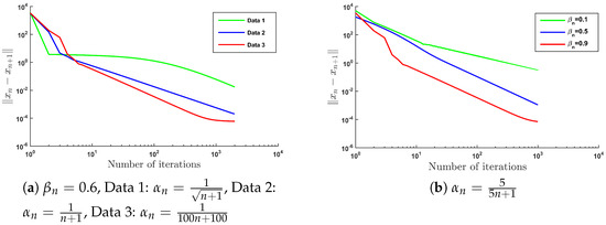
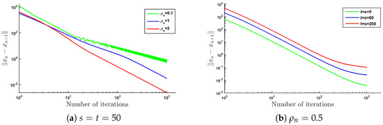
We study the numerical behavior of HSRPA for different parameters ${\alpha }_n$, ${\beta }_n$, ${\rho }_n$ and for different dimensions $s=t$, where $r=2$ (i.e., $N=5$), ${\lambda }_1={\lambda }_2=\frac{1}{2}$, ${\delta }_j=\frac{j}{4}$ for all $j\in \{1,2,3,4\}$ are fixed. Notice that for the choice of ${\lambda }_1={\lambda }_2=\frac{1}{2}$ the parameter ${\rho }_n$ is chosen in such a way that $0<{\rho }_n<4$ and $\underset{n\to \infty }{lim\; inf}{\rho }_n(4-{\rho }_n)>0$. The numerical results are shown in Figure 1 and Figure 2.

Figure 1. For $t=s=100$, ${\rho }_n=2$, $\theta =10$ and for randomly generated starting points $x_1$ and u.

Figure 2. For ${\alpha }_n=\frac{5}{5n+1}$, ${\beta }_n=\frac{1}{2}+\frac{1}{n+4}$, $\theta =150$ and for randomly generated starting points $x_1$ and u.

In view of Figure 1 and Figure 2, we see that our algorithm works better for

(i) 

A sequence $\left\{{\alpha }_n\right\}$ in which the terms are very close to zero;

(ii) 

A sequence $\left\{{\beta }_n\right\}$ in which terms are very close to 1;

(iii) 

A sequence $\left\{{\rho }_n\right\}$ in which terms are larger but not exceeding 4.

Example 2. 

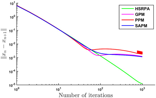
Comparing HSRPA with GPM, PPM and SAPM.

Consider MSSFP (2) for $H_1={\mathbb{R}}^3$, $H_2={\mathbb{R}}^3$, $A:{\mathbb{R}}^3\to {\mathbb{R}}^3$ given by $A=\theta I_{3\times 3}$, the closed convex subsets $C_i$ ($i\in \{1,\dots ,N\}$) of ${\mathbb{R}}^3$ are given by

$$C_i=\left\{x\in {\mathbb{R}}^3:c_i\left(x\right)\le 0\right\},$$

where θ is a real constant, $I_{3\times 3}$ is $3\times 3$ identity matrix and

$$c_i\left(x\right)={(-1)}^i(⟨x,w_i^0⟩-{\gamma }_i)$$

such that $w_i^0={(i,i+1,\frac{i+2}{\sqrt{2}})}^T$ and ${\gamma }_i=5i+3$, and the closed convex subsets $Q_j$ ($j\in \{1,\dots ,M\}$) of ${\mathbb{R}}^3$ are given by

$$Q_j=\left\{y\in {\mathbb{R}}^3:q_j\left(y\right)\le 0\right\},$$

where $q_1\left(y\right)={\parallel y\parallel }^2-12{\theta }^2$, $q_j\left(y\right)={(-1)}^j(⟨y,z_j^0⟩-3\theta (j+j^2))$ and $z_j^0={(j,j^2,\sqrt{2}{j}^2)}^T$ for each $j\in \{2,\cdots ,M\}.$

For each choice of θ the solution set of the MSSFP is $\left\{(3,1,\sqrt{2})\right\}$, i.e., $\overline{x}=(3,1,\sqrt{2})$.

We choose GPM, PPM and SAPM because the problem under consideration is the same and the approach has some common features with our approach.

GPM:The proposed iterative algorithm solving MSSFP is reduced to

$$x_{n+1}=x_n+\varrho \left({\displaystyle \sum _{i=1}^N}{\sigma }_i(P_{C_i}-I)x_n+{\displaystyle \sum _{j=1}^M}{\nu }_j{A}^{\ast }(P_{Q_j}-I)A{x}_n\right),$$

(41)

where $\varrho \in (0,\frac{2}{L})$, $L={\displaystyle \sum _{i=1}^N}{\sigma }_i+\omega {\displaystyle \sum _{j=1}^M}{\nu }_j$ and ${\displaystyle \sum _{i=1}^N}{\sigma }_i+{\displaystyle \sum _{j=1}^M}{\nu }_j=1$ for ${\sigma }_i>0$, ${\nu }_j>0$ and ω is the spectral radius of $A^{\ast }A=A^{t}A$.

PPM:The proposed algorithm is obtained by replacing the projections on the closed convex subset $C_i$ and $Q_j$ in (41) by the half-space $C_{i,n}$ and $C_{j,n}$.

SAPM:The proposed iterative algorithm for solving the MSSFP is reduced to

$$\left\{\begin{array}{c}{y}_n=x_n-{\varrho }_n\nabla p_n\left(x_n\right),\hfill \\ {\varrho }_n=\gamma {\varsigma }^{l_n},wheremin\{l:\parallel \nabla p_n\left(x_n\right)-\nabla p_n\left(y_n\right)\parallel \le \frac{\mu \parallel x_n-y_n\parallel }{\gamma {\varsigma }^l},l=0,1,2,\dots \},\hfill \\ x_{n+1}=x_n-{\varrho }_n\nabla p_n\left(y_n\right),\hfill \end{array}\right.$$

where $\nabla p_n\left(x_n\right)={\displaystyle \sum _{i=1}^N}{\sigma }_i(I-P_{C_{i,n}})x_n+{\displaystyle \sum _{j=1}^M}{\nu }_j{A}^{\ast }(I-P_{Q_{j,n}})A{x}_n$, ${\displaystyle \sum _{i=1}^N}{\sigma }_i+{\displaystyle \sum _{j=1}^M}{\nu }_j=1$ for ${\sigma }_i>0$, ${\nu }_j>0$, $\gamma >0$, $\varsigma \in (0,1)$, $\mu \in (0,1)$.

In our algorithm we took ${\xi }_{i,n}={(-1)}^i{x}_i^0$ for each $i\in \{1,\dots ,N\}$ and

$${\epsilon }_{1,n}=\left\{\begin{array}{cc}\frac{z_n-z_1^0}{\parallel z_n-z_1^0\parallel },\hfill & \hfill if z_n-z_1^0\ne 0,\\ 0,\hfill & \hfill otherwise,\end{array}\right.$$

and ${\epsilon }_{j,n}={(-1)}^j{z}_j^0$ for each $j\in \{2,\cdots ,M\}.$

For the purpose of comparison we took the following data:

HSRPA:${\lambda }_1={\lambda }_2=\frac{1}{2}$, ${\delta }_j=\frac{j}{1+\dots +M}$ for $j\in \{1,\dots ,M\}$, ${\alpha }_n=\frac{1}{n+1}$, ${\beta }_n=\frac{n+2}{2n+6}$, ${\rho }_n=1$.

GPM:$\varrho =\frac{1}{3}$, ${\sigma }_i=\frac{i}{2(1+\dots +N)}$ for $i\in \{1,\cdots ,N\}$, ${\nu }_j=\frac{j}{2(1+\dots +M)}$ for $j\in \{1,\dots ,M\}$.

PPM:$\varrho =\frac{1}{3}$, ${\sigma }_i=\frac{i}{2(1+\dots +N)}$ for $i\in \{1,\cdots ,N\}$, ${\nu }_j=\frac{j}{2(1+\dots +M)}$ for $j\in \{1,\dots ,M\}$.

SAPM:$\gamma =1$, $\varsigma =\frac{1}{2}=\mu$, ${\sigma }_i=\frac{i}{2(1+\dots +N)}$ for $i\in \{1,\cdots ,N\}$, ${\nu }_j=\frac{j}{2(1+\dots +M)}$ for $j\in \{1,\dots ,M\}$.

The numerical results are shown in Table 1 and Figure 3. To permit comparisons between the three algorithms about the number of iterations (Iter(n)) and the time of execution in seconds (CPUt(s)), we have used the relative difference $\frac{\parallel x_n-x_{n+1}\parallel }{\parallel x_1-u\parallel }$, which is less than ϵ, as the stopping criteria in Table 1.

Table 1. For $\theta =3$, $u=(4,-6,9)$ and $x_1=(-4,7,-19)$.

			$\mathit{ϵ}={10}^{-2}$,$\mathit{N}=3$,$\mathit{M}=2$		$\mathit{ϵ}={10}^{-3}$,$\mathit{N}=4=\mathit{M}$
	Iter(n)		271		359
HSRPA	CPUt(s)		$2.478534$		$2.7094060$
	$\parallel x_n-\overline{x}\parallel$		$1.29153127891261\times {10}^{-11}$		$3.95548438843874\times {10}^{-5}$
	Iter(n)		286		421
GPM	CPUt(s)		$2.350976$		$3.0921890$
	$\parallel x_n-\overline{x}\parallel$		$1.32185889807060\times {10}^{-11}$		$4.00584274497442\times {10}^{-5}$
	Iter(n)		293		368
PPM	CPUt(s)		$2.462534$		$2.6903446$
	$\parallel x_n-\overline{x}\parallel$		$1.34325049285599\times {10}^{-11}$		$3.97217074806315\times {10}^{-5}$
	Iter(n)		277		397
SAPM	CPUt(s)		$2.192005$		$2.6393334$
	$\parallel x_n-\overline{x}\parallel$		$1.30707774298130\times {10}^{-11}$		$4.0068355895327\times {10}^{-5}$

Figure 3. For $N=50$ and starting points $u=(-1,\dots ,-1)\in {\mathbb{R}}^N$ (in HSRPA) and $x_1=-2u$.

From the numerical results in Table 1 and Figure 3 of Example 2, we can see that our algorithm (HSRPA) has better performance than GPM, PPM and SAPM. To be specific, HSRPA converges faster and requires less iterations than GPM, PPM and SAPM. In view of CPU time of execution, our algorithm has comparable performance with GPM, PPM and SAPM.

Example 3. 

Consider the MSSFP with $H_1={\mathbb{R}}^s,H_2={\mathbb{R}}^t$ and $C_i=\{x\in {\mathbb{R}}^s:-5i{e}_1\le x\le (N-i)e_1\}$ ($i\in \{1,\dots ,N\}$) and $Q_j=\{y\in {\mathbb{R}}^t:(j-M)e_1\le y\le j{e}_1\},$ ($j\in \{1,\dots ,M\}$), with a different number of feasible sets N and M, and dimensions s and t. We randomly generated the operator $A={\left(a_{ij}\right)}_{t\times s}$, with $a_{ij}\in [0,10].$ In this example, we see the effect of the different choices of ${\lambda }_1$ and ${\lambda }_2$ for the numerical results of the HSRPA using both stepsizes ${\tau }_{j,n}$ and ${\tau }_{j,n}^{\ast }$ (given in (38)), and also we compare the HSRPA with the algorithm proposed by Zhao et al. ([48], Algorithm 2.1). For the HSRPA we take $u={(1,1,2)}^T,x_1=rand[-100,100]$, $N=3,M=10,s=t=3$, ${\rho }_n=3$, ${\alpha }_n=\frac{1}{n+1}$, ${\beta }_n=\frac{n+5}{2n+6}$ and ${\delta }_j=\frac{j}{1+\dots +M}$, $j\in \{1,\dots ,M\}$. For ([48], Algorithm 2.1), we take $x^0=rand[-100,100]$, $t=3,r=10,N=M=3$, ${\omega }_k=1$, ${\alpha }_i={\left(\frac{1013}{3000}\right)}^i$, $i=1,2,3$, and ${\beta }_j={\left(\frac{1013}{3000}\right)}^j$, $j=1,2,\cdots ,10$. We use $\parallel x_{n+1}-x_n\parallel <{10}^{-4}$ as the stopping criteria. The results are presented in Table 2 below.

Table 2. Comparative result of the Half-Space Relaxation Projection Algorithm (HSRPA) (with two different stepsizes ${\tau }_{j,n}$ and ${\tau }_{j,n}^{\ast }$) with ([48], Algorithm 2.1) for different choices of ${\lambda }_1$ and ${\lambda }_2.$

Choices of ${\mathit{\lambda }}_1,{\mathit{\lambda }}_2$	HSRPA (${\mathit{\tau }}_{\mathit{j},\mathit{n}}$)		HSRPA (${\mathit{\tau }}_{\mathit{j},\mathit{n}}^{\ast }$)		Algorithm 2.1
	Ite.	CPUt(s)	Ite.	CPUt(s)	Ite.	CPUt(s)
${\lambda }_1=0.9,{\lambda }_2=0.1$	56	8.9971	51	7.3628	235	28.7590
${\lambda }_1=0.8,{\lambda }_2=0.2$	55	5.8883	37	3.7528
${\lambda }_1=0.7,{\lambda }_2=0.3$	45	4.7402	39	3.9150
${\lambda }_1=0.6,{\lambda }_2=0.4$	42	4.6510	38	3.9080
${\lambda }_1=0.5,{\lambda }_2=0.5$	38	3.9295	45	4.5573
${\lambda }_1=0.4,{\lambda }_2=0.6$	36	3.1803	44	4.4400
${\lambda }_1=0.3,{\lambda }_2=0.7$	42	4.3067	50	5.0784
${\lambda }_1=0.2,{\lambda }_2=0.8$	29	3.4536	36	3.8640
${\lambda }_1=0.1,{\lambda }_2=0.9$	32	3.3220	38	4.1409

Interestingly, it can be observed from Table 2 that, for ${\lambda }_1\le {\lambda }_2$ HSRPA with the stepsize ${\tau }_{j,n}$ is faster in terms of less number of iterations and CPU-run time than HSRPA with the stepsize ${\tau }_{j,n}^{\ast }$. On the contrary, HSRPA (${\tau }_{j,n}^{\ast }$) has better performance for ${\lambda }_1>{\lambda }_2$ and HSRPA with either of the stepsizes converges faster and requires less number of iterations than the compared algorithm ([48], Algorithm 2.1).

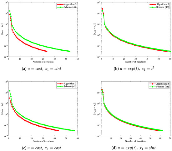
Example 4. 

Consider the Hilbert space $H_1=H_2=L^2\left([0,1]\right)$ with norm $\parallel x\left|\right|:=\sqrt{{\int }_0^1{\left|x\left(t\right)\right|}^{2}dt}$ and the inner product given by $⟨x,y⟩={\int }_0^{1}x\left(t\right)y\left(t\right)dt$. The two nonempty, closed and convex sets are $C=\{x\in L^2\left([0,1]\right):⟨x\left(t\right),3t^2⟩=0\}$ and $Q=\{x\in L^2\left([0,1]\right):⟨x,\frac{t}{3}⟩\ge -1\}$, and the linear operator is given as $\left(Ax\right)\left(t\right)=x\left(t\right)$, i.e., $\parallel A\parallel =1$ or $A=I$ is the identity. The orthogonal projection onto C and Q have an explicit formula; see, for example, [57]

$$P_C\left(w\left(t\right)\right)=\left\{\begin{array}{c}w\left(t\right)-\frac{⟨w\left(t\right),3t^2⟩}{\parallel 3t^2{\parallel }_{L^2}^2}3t^2,if⟨w\left(t\right),3t^2⟩\ne 0,\hfill \\ w\left(t\right),if⟨w\left(t\right),3t^2⟩=0.\hfill \end{array}\right.$$

$$P_Q\left(w\left(t\right)\right)=\left\{\begin{array}{c}w\left(t\right)-\frac{⟨w\left(t\right),\frac{-t}{3}⟩-1}{\parallel \frac{-t}{3}{\parallel }_{L^2}^2}\left(\frac{-t}{3}\right),if⟨w\left(t\right),\frac{-t}{3}⟩<-1,\hfill \\ w\left(t\right),if⟨w\left(t\right),\frac{-t}{3}⟩\ge -1.\hfill \end{array}\right.$$

We consider the following problem

$$find{x}^{\ast }\in CsuchthatA{x}^{\ast }\in Q.$$

(42)

It is clear that Problem (42) has a nonempty solution set Ω since $0\in \mathsf{\Omega }$. In this case, the iterative scheme in Algorithm 2($u,x_1\in C,$ with ${\lambda }_1={\lambda }_2=\frac{1}{2},{\rho }_n=\frac{7}{2},{\alpha }_n=\frac{1}{n+1},and{\beta }_n=\frac{n+2}{2n+6}$) becomes

$$\left\{\begin{array}{c}{z}_n=(1-\frac{1}{n+1})x_n+\frac{u}{n+1},\hfill \\ y_n=z_n-\frac{{\tau }_n}{2}((I-P_{C_n})z_n+A^{\ast }(I-P_{Q_n})A{z}_n),\hfill \\ x_{n+1}=(1-\frac{n+2}{2n+6})z_n+\left(\frac{n+2}{2n+6}\right)y_n,\hfill \end{array}\right.$$

where

$${\tau }_n=\frac{7(\parallel (I-P_{C_n})z_n{\parallel }^2+\parallel (I-P_{Q_n})A{z}_n{\parallel }^2)}{d\left(z_n\right)},$$

for

$$d\left(z_n\right)=\left\{\begin{array}{c}1,if\parallel (I-P_{C_n})z_n{\parallel }^2+{\parallel A^{\ast }(I-P_{Q_n})A{z}_n\parallel }^2=0\hfill \\ \parallel (I-P_{C_n})z_n{\parallel }^2+{\parallel A^{\ast }(I-P_{Q_n})A{z}_n\parallel }^2,otherwise.\hfill \end{array}\right.$$

In this example, we compare Algorithm 2 with the strong convergence result of SFP proposed by Shehu et al. [56]. The iterative scheme (27) in [56] for $u,x_1\in C,$ with ${\alpha }_n=\frac{1}{n+1}$, ${\beta }_n=\frac{n}{2(n+1)}={\gamma }_n$ and $t_n=\frac{1}{{\parallel A\parallel }^2}$ was reduced into the following form

$$\left\{\begin{array}{c}{y}_n=[x_n-\frac{1}{{\parallel A\parallel }^2}{A}^{\ast }(A{x}_n-P_{Q_n}\left(A{x}_n\right))]\hfill \\ x_{n+1}=P_C\left(\frac{u}{n+1}+\frac{n{x}_n}{2(n+1)}+\frac{n{y}_n}{2(n+1)}\right),n\ge 1.\hfill \end{array}\right.$$

(43)

We see here that our iterative scheme can be implemented to solve the problem (42) considered in this example. We use $\parallel x_{n+1}-x_n\parallel <{10}^{-3}$ as stopping criteria for both algorithms and the outcome of the numerical experiment is reported in Figure 4. It can be observed from Figure 4 that, for different choices of u and $x_1$, Algorithm 2 is faster in terms of less number of iterations and CPU-run time than the algorithm proposed by Shehu et al. [56].

Figure 4. Comparison of Algorithm 2 and algorithm by Shehu [56] for different choices of u and $x_1$.

4.1. Application to Signal Recovery

In this part, we consider the problem of recovering a noisy sparse signal. Compressed sensing can be modeled as the following linear equation:

$$b=Ax+ϵ,$$

(44)

where $x\in {\mathbb{R}}^N$ is a vector with L nonzero components to be recovered, $b\in {\mathbb{R}}^M$ is the measured data with noisy $ϵ$ (when $ϵ=0,$ it means that there is no noise to the observed data) and A is an $M\times N$ bounded linear observation operator with ($N>M$). The problem in Equation (44) can be seen as the LASSO problem, which has wide application in signal processing theory [58].

$$\begin{array}{cc}\hfill & \underset{x\in {\mathbb{R}}^N}{min}\frac{1}{2}{\parallel Ax-b\parallel }_2^2\hfill \\ \hfill & {\mathrm{subject}\mathrm{to}\parallel x\parallel }_1\le t,\hfill \end{array}$$

(45)

where $t>0$ is a given constant. It can be observed that (45) indicates the potential of finding a sparse solution of the SFP (3) due to the ${\ell }_1$ constraint. Thus, we apply Algorithm 2 to solve problem (45).

Let $C:=\{x:\parallel x{\parallel }_1\le t\}$ and $Q=\left\{b\right\},$ then the minimization problem (45) can be seen as an SFP (3). Denote the level set $C_n$ by,

$$C_n=\{x\in {\mathbb{R}}^N:\omega \left(x_n\right)+⟨{\varsigma }_n,x-x_n⟩\le 0\},$$

(46)

where ${\varsigma }_n\in \partial \omega \left(x_n\right)$ with the convex function $\omega \left(x\right)={\parallel x\parallel }_1-t$.

For a special case where $Q=Q_n=\left\{b\right\},$ Algorithm 2 converges to the solution of (45) and moreover, since the projection onto the level set has an explicit formula, Algorithm 2 can be easily implemented. In the sequel, we present a sparse signal recovery experiment to illustrate the efficiency of Algorithm 2 by comparing with algorithms proposed by Lopez [2] and Yang [37].

The vector x is an $L-$sparse signal with L non-zero elements that is generated from uniform distribution in the interval $[-2,2]$. The matrix A is generated from a normal distribution with mean zero and one variance. The observation b is generated by white Gaussian noise with signal-to-noise ratio $SNR=40$. The process is started with $t=L$, $x_0$ and u are randomly generated $N\times 1$ vectors. The goal is then to recover the $L-$sparse signal x by solving (45). The restoration accuracy is measured by the mean squared error as follows:

$$MSE=\frac{1}{N}\parallel x_{n+1}-x_n\parallel \le ϵ,$$

(47)

where $x_n$ is an estimated signal of x, and $ϵ>0$ is a given small constant. We take the stopping criteria $ϵ={10}^{-6}$ and we choose the corresponding parameters ${\rho }_n=3.5,{\lambda }_1={\lambda }_2=0.5$ for Algorithm 2. We also choose $\gamma =\frac{1}{{\parallel A\parallel }^2}$ and ${\rho }_n=2$ for the algorithm by Yang [37] and algorithm by Lopez [2], respectively.

It can be observed from Figure 5, Figure 6, Figure 7 and Figure 8 that the recovered signal by the proposed algorithm has less number of iterations and MSE. Therefore, the quality of the signal recovered by the proposed algorithm is better than the compared algorithms.

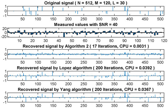
Figure 5. The original $L-$sparse signal versus the recovered sparse signal by Algorithm 2, algorithms by Lopez [2] and Yang [37] when $N=512,$ $M=120$ and $L=30$.

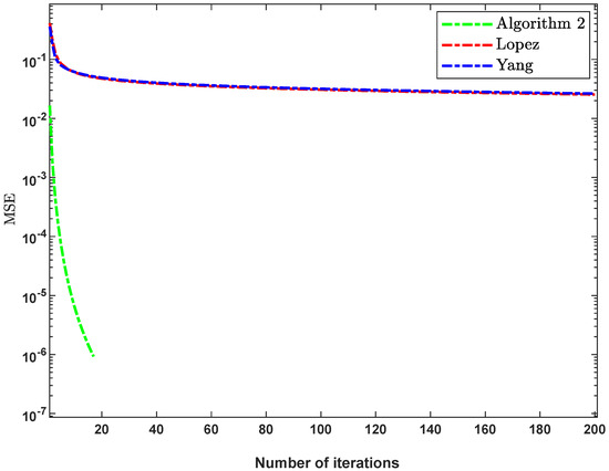
Figure 6. MSE versus the number of iterations, and the comparison of Algorithm 2 with that of algorithms by Lopez [2] and Yang [37] when $N=512,$$M=120$ and $L=30$.

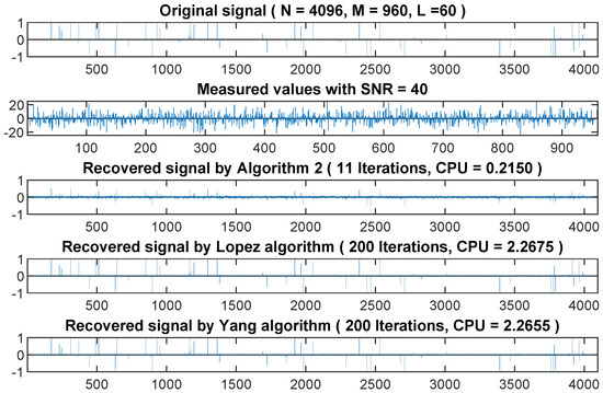
Figure 7. The original $L-$sparse signal versus the recovered sparse signal by Algorithm 2, algorithms by Lopez [2] and Yang [37] when $N=4096,$$M=960$ and $L=60$.

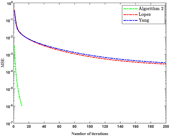
Figure 8. MSE versus the number of iterations, and the comparison of Algorithm 2 with that of algorithms by Lopez [2] and Yang [37] when $N=4096,$$M=960$ and $L=60$.

5. Conclusions

In this paper, we present a strong convergence iterative algorithm solving MSSFP with a way of selecting the stepsizes such that the implementation of the algorithm does not need any prior information as regards the operator norms. Preliminary numerical results are reported to illustrate the numerical behavior of our algorithm (HSRPA), and to compare it with those well known in the literature, including, Censor et al. ([7], Algorithm 1), Censor et al. ([43], Algorithm 5), Zhao and Yang ([46], Algorithm 3.2) and Zhao et al. ([48], Algorithm 2.1). The numerical results show that our proposed Algorithm is practical and promising for solving MSSFP. Algorithm 2 is applied in signal recovery. The experiment results show that Algorithm 2 has fewer iterations than that of algorithms proposed by Yang [37], Lopez [2] and Shehu [56].

References

- Censor, Y.; Gibali, A.; Reich, S. Algorithms for the split variational inequality problem. Numer. Algorithms 2012, 59, 301–323. [Google Scholar] [CrossRef]
- López, G.; Martín-Márquez, V.; Wang, F.; Xu, H.K. Solving the split feasibility problem without prior knowledge of matrix norms. Inverse Probl. 2012, 28, 085004. [Google Scholar] [CrossRef]
- Byrne, C. A unified treatment of some iterative algorithms in signal processing and image reconstruction. Inverse Probl. 2003, 20, 103. [Google Scholar] [CrossRef]
- Combettes, P. The convex feasibility problem in image recovery. In Advances in Imaging and Electron Physics; Elsevier: Amsterdam, The Netherlands, 1996; Volume 95, pp. 155–270. [Google Scholar]
- Qu, B.; Xiu, N. A note on the CQ algorithm for the split feasibility problem. Inverse Probl. 2005, 21, 1655. [Google Scholar] [CrossRef]
- Censor, Y.; Elfving, T. A multiprojection algorithm using Bregman projections in a product space. Numer. Algorithms 1994, 8, 221–239. [Google Scholar] [CrossRef]
- Censor, Y.; Elfving, T.; Kopf, N.; Bortfeld, T. The multiple-sets split feasibility problem and its applications for inverse problems. Inverse Probl. 2005, 21, 2071. [Google Scholar] [CrossRef]
- Censor, Y.; Lent, A. Cyclic subgradient projections. Math. Program. 1982, 24, 233–235. [Google Scholar] [CrossRef]
- Byrne, C.; Censor, Y.; Gibali, A.; Reich, S. The split common null point problem. arXiv 2011, arXiv:1108.5953. [Google Scholar]
- Censor, Y.; Segal, A. The split common fixed point problem for directed operators. J. Convex Anal. 2009, 16, 587–600. [Google Scholar]
- Dang, Y.; Gao, Y.; Li, L. Inertial projection algorithms for convex feasibility problem. J. Syst. Eng. Electron. 2012, 23, 734–740. [Google Scholar] [CrossRef]
- He, Z. The split equilibrium problem and its convergence algorithms. J. Inequalities Appl. 2012, 2012, 162. [Google Scholar] [CrossRef]
- Taiwo, A.; Jolaoso, L.O.; Mewomo, O.T. Viscosity approximation method for solving the multiple-set split equality common fixed-point problems for quasi-pseudocontractive mappings in Hilbert spaces. J. Ind. Manag. Optim. 2017, 13. [Google Scholar] [CrossRef]
- Aremu, K.O.; Izuchukwu, C.; Ogwo, G.N.; Mewomo, O.T. Multi-step iterative algorithm for minimization and fixed point problems in p-uniformly convex metric spaces. J. Manag. Optim. 2017, 13. [Google Scholar] [CrossRef]
- Oyewole, O.K.; Abass, H.A.; Mewomo, O.T. A strong convergence algorithm for a fixed point constrained split null point problem. Rend. Circ. Mat. Palermo Ser. 2 2020, 13, 1–20. [Google Scholar]
- Izuchukwu, C.; Ugwunnadi, G.C.; Mewomo, O.T.; Khan, A.R.; Abbas, M. Proximal-type algorithms for split minimization problem in P-uniformly convex metric spaces. Numer. Algorithms 2019, 82, 909–935. [Google Scholar] [CrossRef]
- Jolaoso, L.O.; Alakoya, T.O.; Taiwo, A.; Mewomo, O.T. Inertial extragradient method via viscosity approximation approach for solving equilibrium problem in Hilbert space. Optimization 2020, 1–20. [Google Scholar] [CrossRef]
- He, S.; Wu, T.; Cho, Y.J.; Rassias, T.M. Optimal parameter selections for a general Halpern iteration. Numer. Algorithms 2019, 82, 1171–1188. [Google Scholar] [CrossRef]
- Dadashi, V.; Postolache, M. Forward–backward splitting algorithm for fixed point problems and zeros of the sum of monotone operators. Arab. J. Math. 2020, 9, 89–99. [Google Scholar] [CrossRef]
- Yao, Y.; Leng, L.; Postolache, M.; Zheng, X. Mann-type iteration method for solving the split common fixed point problem. J. Nonlinear Convex Anal. 2017, 18, 875–882. [Google Scholar]
- Byrne, C. Iterative oblique projection onto convex sets and the split feasibility problem. Inverse Probl. 2002, 18, 441. [Google Scholar] [CrossRef]
- Dang, Y.; Gao, Y. The strong convergence of a KM–CQ-like algorithm for a split feasibility problem. Inverse Probl. 2010, 27, 015007. [Google Scholar] [CrossRef]
- Jung, J.S. Iterative algorithms based on the hybrid steepest descent method for the split feasibility problem. J. Nonlinear Sci. Appl. 2016, 9, 4214–4225. [Google Scholar] [CrossRef]
- Wang, F.; Xu, H.K. Cyclic algorithms for split feasibility problems in Hilbert spaces. Nonlinear Anal. Theory Methods Appl. 2011, 74, 4105–4111. [Google Scholar] [CrossRef]
- Xu, H.K. An iterative approach to quadratic optimization. J. Optim. Theory Appl. 2003, 116, 659–678. [Google Scholar] [CrossRef]
- Xu, H.K. A variable Krasnosel’skii–Mann algorithm and the multiple-set split feasibility problem. Inverse Probl. 2006, 22, 2021. [Google Scholar] [CrossRef]
- Xu, H.K. Iterative methods for the split feasibility problem in infinite-dimensional Hilbert spaces. Inverse Probl. 2010, 26, 105018. [Google Scholar] [CrossRef]
- Yu, X.; Shahzad, N.; Yao, Y. Implicit and explicit algorithms for solving the split feasibility problem. Optim. Lett. 2012, 6, 1447–1462. [Google Scholar] [CrossRef]
- Shehu, Y.; Mewomo, O.T.; Ogbuisi, F.U. Further investigation into approximation of a common solution of fixed point problems and split feasibility problems. Acta Math. Sci. 2016, 36, 913–930. [Google Scholar] [CrossRef]
- Shehu, Y.; Mewomo, O.T. Further investigation into split common fixed point problem for demicontractive operators. Acta Math. Sin. Engl. Ser. 2016, 32, 1357–1376. [Google Scholar] [CrossRef]
- Mewomo, O.T.; Ogbuisi, F.U. Convergence analysis of an iterative method for solving multiple-set split feasibility problems in certain Banach spaces. Quaest. Math. 2018, 41, 129–148. [Google Scholar] [CrossRef]
- Dong, Q.L.; Tang, Y.C.; Cho, Y.J.; Rassias, T.M. “Optimal” choice of the step length of the projection and contraction methods for solving the split feasibility problem. J. Glob. Optim. 2018, 71, 341–360. [Google Scholar] [CrossRef]
- Cegielski, A. Landweber-type operator and its properties. Contemp. Math. 2016, 658, 139–148. [Google Scholar]
- Cegielski, A. General method for solving the split common fixed point problem. J. Optim. Theory Appl. 2015, 165, 385–404. [Google Scholar] [CrossRef]
- Cegielski, A.; Reich, S.; Zalas, R. Weak, strong and linear convergence of the CQ-method via the regularity of Landweber operators. Optimization 2020, 69, 605–636. [Google Scholar] [CrossRef]
- Hendrickx, J.M.; Olshevsky, A. Matrix p-norms are NP-hard to approximate if p ≠ 1,2,∞. SIAM J. Matrix Anal. Appl. 2010, 31, 2802–2812. [Google Scholar] [CrossRef]
- Yang, Q. The relaxed CQ algorithm solving the split feasibility problem. Inverse Probl. 2004, 20, 1261. [Google Scholar] [CrossRef]
- Bauschke, H.H.; Borwein, J.M. On projection algorithms for solving convex feasibility problems. SIAM Rev. 1996, 38, 367–426. [Google Scholar] [CrossRef]
- Fukushima, M. A relaxed projection method for variational inequalities. Math. Program. 1986, 35, 58–70. [Google Scholar] [CrossRef]
- Alakoya, T.O.; Jolaoso, L.O.; Mewomo, O.T. Modified inertial subgradient extragradient method with self adaptive stepsize for solving monotone variational inequality and fixed point problems. Optimization 2020, 1–30. [Google Scholar] [CrossRef]
- Jolaoso, L.O.; Taiwo, A.; Alakoya, T.O.; Mewomo, O.T. A unified algorithm for solving variational inequality and fixed point problems with application to the split equality problem. Comput. Appl. Math. 2020, 39, 38. [Google Scholar] [CrossRef]
- Buong, N. Iterative algorithms for the multiple-sets split feasibility problem in Hilbert spaces. Numer. Algorithms 2017, 76, 783–798. [Google Scholar] [CrossRef]
- Censor, Y.; Motova, A.; Segal, A. Perturbed projections and subgradient projections for the multiple-sets split feasibility problem. J. Math. Anal. Appl. 2007, 327, 1244–1256. [Google Scholar] [CrossRef]
- Latif, A.; Vahidi, J.; Eslamian, M. Strong convergence for generalized multiple-set split feasibility problem. Filomat 2016, 30, 459–467. [Google Scholar] [CrossRef]
- Masad, E.; Reich, S. A note on the multiple-set split convex feasibility problem in Hilbert space. J. Nonlinear Convex Anal. 2007, 8, 367. [Google Scholar]
- Zhao, J.; Yang, Q. Self-adaptive projection methods for the multiple-sets split feasibility problem. Inverse Probl. 2011, 27, 035009. [Google Scholar] [CrossRef]
- Zhao, J.; Yang, Q. Several acceleration schemes for solving the multiple-sets split feasibility problem. Linear Algebra Appl. 2012, 437, 1648–1657. [Google Scholar] [CrossRef][Green Version]
- Zhao, J.; Yang, Q. A simple projection method for solving the multiple-sets split feasibility problem. Inverse Probl. Sci. Eng. 2013, 21, 3537–3546. [Google Scholar] [CrossRef]
- Yao, Y.; Postolache, M.; Zhu, Z. Gradient methods with selection technique for the multiple-sets split feasibility problem. Optimization 2019, 69, 269–281. [Google Scholar] [CrossRef]
- Osilike, M.O.; Isiogugu, F.O. Weak and strong convergence theorems for nonspreading-type mappings in Hilbert spaces. Nonlinear Anal. Theory Methods Appl. 2011, 74, 1814–1822. [Google Scholar] [CrossRef]
- Aubin, J.P. Optima and Equilibria: An Introduction to Nonlinear Analysis; Springer Science & Business Media: Berlin, Germany, 2013; Volume 140. [Google Scholar]
- Ceng, L.C.; Ansari, Q.H.; Yao, J.C. An extragradient method for solving split feasibility and fixed point problems. Comput. Math. Appl. 2012, 64, 633–642. [Google Scholar] [CrossRef]
- Bauschke, H.H.; Combettes, P.L. Convex Analysis and Monotone Operator Theory in Hilbert Spaces; Springer: Berlin/Heidelberg, Germany, 2011; Volume 408. [Google Scholar]
- Maingé, P.E.; Măruşter, Ş. Convergence in norm of modified Krasnoselski–Mann iterations for fixed points of demicontractive mappings. Appl. Math. Comput. 2011, 217, 9864–9874. [Google Scholar] [CrossRef]
- He, B. Inexact implicit methods for monotone general variational inequalities. Math. Program. 1999, 86, 199–217. [Google Scholar] [CrossRef]
- Shehu, Y. Strong convergence result of split feasibility problems in Banach spaces. Filomat 2017, 31, 1559–1571. [Google Scholar] [CrossRef][Green Version]
- Cegielski, A. Iterative Methods for Fixed Point Problems in Hilbert Spaces; Springer: Berlin/Heidelberg, Germany, 2012; Volume 2057. [Google Scholar]
- Gibali, A.; Liu, L.W.; Tang, Y.C. Note on the modified relaxation CQ algorithm for the split feasibility problem. Optim. Lett. 2018, 12, 817–830. [Google Scholar] [CrossRef]
© 2020 by the authors. Licensee MDPI, Basel, Switzerland. This article is an open access article distributed under the terms and conditions of the Creative Commons Attribution (CC BY) license (http://creativecommons.org/licenses/by/4.0/).