Numerical Solution for Fuzzy Enzyme Kinetic Equations by the Runge–Kutta Method

Abstract

One of the most important biochemical reactions is catalyzed by enzymes. A numerical method to solve nonlinear equations of enzyme kinetics, known as the Michaelis and Menten equations, together with fuzzy initial values is introduced. The numerical method is based on the fourth order Runge–Kutta method, which is generalized for a fuzzy system of differential equations. The convergence and stability of the method are also presented. The capability of the method in fuzzy enzyme kinetics is demonstrated by some numerical examples.

1. Introduction

Enzymes found in nature have been used since ancient times in the production of food products. Enzymes are currently used in several different industrial products and processes. In a world with a rapidly-increasing population and approaching the exhaustion of many natural resources, enzyme technology offers a great potential for many industries to help meet the challenges they will face in years to come [1]. Enzymes are among the catalysts for chemical reactions. Most enzymes are proteins, although a few are RNAs. Enzymes help substrate molecules become products. Enzymes can multiply the speed of a reaction up to a million times. Without enzymes, many of the reactions become slow or impossible [2,3,4,5]. Enzyme kinetics deals with the study of reactions that are performed by enzymes. In 1913, Michaelis and Menten offered a simple model for enzyme reaction, as seen below [3,5,6]. Suppose E is the enzyme and S is the substrate, and their combination is C. C irreversibly becomes an enzyme and the product P, that is:

$$E+S\to C\to E+P$$

Using the concepts of mass action and the mass conservation law, we get to the system of differential equations. For simplicity, we will use the same symbols $C,S,E$ and P to refer to both the chemicals $C,S,E$ and P and their concentrations.

$$\left\{\begin{array}{c}\begin{array}{c}\frac{dE}{dt}=-{\eta }_{0}ES+({\eta }_1+{\eta }_2)C,\hfill \\ \frac{dS}{dt}=-{\eta }_{0}ES+{\eta }_{1}C,\hfill \\ \frac{dC}{dt}={\eta }_{0}ES-({\eta }_1+{\eta }_2)C,\hfill \\ \frac{dP}{dt}={\eta }_{2}C,\hfill \end{array}\end{array}\right.$$

(1)

where ${\eta }_0,{\eta }_1$ and ${\eta }_2$ are the rates of the reaction constants; together with initial conditions $S(0)=S_0$, $E(0)=E_0,C(0)=C_0$ and $P(0)=0$. These initial conditions are physically supported in the sense that, if no reaction takes place, we cannot have a product. From Equation (1), we have:

$$\begin{array}{c}\hfill {\displaystyle \frac{d(E+C)}{dt}}=0⟹E+C=E_0⟹E=E_0-C\end{array}$$

Hence, Equation (1) can be written as follows:

$$\left\{\begin{array}{c}\begin{array}{c}\frac{dC}{dt}=f_1(t,C,S)=\lambda S(t)-(\theta +{\eta }_{0}S(t))C(t),\hfill \\ \frac{dS}{dt}=f_2(t,C,S)=-\lambda S(t)+({\eta }_{0}S(t)+{\eta }_1)C(t),\hfill \\ C(0)=C_0,S(0)=S_0\hfill \end{array}\end{array}\right.$$

(2)

where $\theta ={\eta }_1+{\eta }_2$ and $\lambda ={\eta }_0{E}_0$.

Various numerical methods to solve Equation (1) have been offered. Sen in [7] applied the Adomian decomposition method; Khader in [8] applied the Picard–Pade technique; and Batiha and Batiha in [9] applied the differential transformation method. In the present study, the numerical solutions of enzyme kinetic Equation (2) are studied by introducing a new fuzzy enzyme kinetic models in a way that the initial conditions are fuzzy numbers.

The concept of fuzzy mathematics was first introduced by Zadeh [10]. Then, many researchers developed it in many different areas, including fuzzy differential equations. The theoretical framework of the fuzzy initial value problem (FIVP) has been an active research field over the last few years. The concept of the fuzzy derivative was first introduced by Chang and Zadeh in [11]. This was followed up by Dubois and Prade in [12], who defined and used the extension principle. A comprehensive approach to FIVPs has been given in the work of Seikkala [13] and Kaleva [14,15], especially in its generalized form given by Buckly and Feuring [16]. Their work is important as it overcomes the existence of multiple definitions of the derivative of fuzzy functions; see [12,13,17,18,19]. Furthermore, [16] compares the various solutions to the FIVP that one may obtain using the different derivatives. Nieto [20] considered the Cauchy problem for continuous fuzzy differential equations (FDEs). The generalized fuzzy differentiability was suggested more recently by Stefanini and Bede [21].

Fuzzy differential equations can be used as a model to describe the phenomenon that includes uncertainty parameters. The results of [13] on a certain category of fuzzy differential equations (FDEs) have inspired several authors who have applied numerical methods for the solution of these equations. The most important contribution to these numerical methods is the Euler method provided by Ma, Friedman and Kandel in [18]. Abbasbandy and Viranloo in [22,23] developed fourth order Runge–Kutta methods for a Cauchy problem with a fuzzy initial value and fuzzy differential equations of order n. Furthermore, in [24], the authors applied Runge–Kutta methods to a more general category of problems, and they proved convergence for s-stage Runge–Kutta methods. The basics of various approaches of FDEs can be found in [25].

The organization of the paper is as follows: In Section 2, some basic results from the fourth order Runge–Kutta method and the fuzzy numbers are presented. In Section 3, the system of fuzzy initial value problems is discussed. In Section 4, the numerical solution of the fuzzy enzyme kinetic equations through the fourth order Runge–Kutta method is illustrated. The convergence and stability of the method are presented in Section 5. Some numerical cases are introduced by an example in Section 6. Finally, the conclusion is given in Section 7.

2. Preliminaries

Given the initial value problem (IVP):

$$\left\{\begin{array}{cc}\hfill y^{\prime }=f(t,y),& a\le t\le b\\ \hfill y(a)=y_a.& \end{array}\right.$$

(3)

The fourth order Runge–Kutta method [26] is as follows:

$$\left\{\begin{array}{c}\begin{array}{c}{k}_1=f(t_i,y_i),\hfill \\ k_2=f(t_i+\frac{h}{2},y_{i+}\frac{h}{2}{k}_1),\hfill \\ k_3=f(t_i+\frac{h}{2},y_{i+}\frac{h}{2}{k}_2),\hfill \\ k_4=f(t_i+h,y_{i+}h{k}_3),\hfill \\ y_{i+1}=y_i+\frac{h}{6}(k_1+2k_2+2k_3+k_4),\hfill \end{array}\end{array}\right.$$

(4)

where $a=t_0\le t_1\le \dots \le t_N=b,h=\frac{(b-a)}{N}=t_{i+1}-t_i$ and $i=0,1,\dots ,N-1$.

In this part, some definitions and the necessary fuzzy mathematics (see [17]) are reviewed.

The set of all real numbers is denoted by $\mathbb{R}$, and the set of all fuzzy numbers on $\mathbb{R}$ is denoted by ${\mathbb{R}}_F$. A fuzzy number is a mapping $\omega :\mathbb{R}\to [0,1]$ with the following properties:

(a)

$\omega$ is upper semi-continuous on $\mathbb{R}$.

(b)

$\omega$ is fuzzy convex, i.e., for $0\le \lambda \le 1$ and any $x,y\in \mathbb{R},$ $\omega (\lambda x+(1-\lambda )y)\ge \mathit{min}\{\omega (x),\omega (y)\}$.

(c)

$\omega$ is normal, i.e., $\exists x_0\in \mathbb{R}$ for which $\omega (x_0)=1$.

(d)

${\left[\omega \right]}^0=cl\{x\in \mathbb{R}:\omega (x)>0\}$ is the support of $\omega$, and its closure is compact.

For $r\in (0,1],$ define ${\left[\omega \right]}_r=\{x\in \mathbb{R}:\omega (x)\ge r\}=[\underline{\omega }(r),\overline{\omega }(r)]$.

Then from (a)–(d), it follows that for all $r\in [0,1]$, the r-level set ${\left[\omega \right]}_r$ is a closed bounded interval.

Let I be a real interval; a mapping $\omega :I\to {\mathbb{R}}_F$ is called a fuzzy process, and its r-level set is denoted by:

$$\omega (t;r)=[\underline{\omega }(t;r),\overline{\omega }(t;r)],t\in I,r\in [0,1].$$

We can define a triangular fuzzy number $\omega$ by three real numbers $v_1\le v_2\le v_3$ where the graph of $\omega (x),$ the membership function of the fuzzy number $\omega =(v_1,v_2,v_3)$, is a triangle with the base on the interval $v_1,v_3$ and the vertex at $x=v_2$. A triangular fuzzy number $\omega =(v_1,v_2,v_3)$ can be written as $\alpha$-cut for $r\in [0,1]$ as $\underline{\omega }(r)=v_1+(v_2-v_1)r$ and $\overline{\omega }(r)=v_1+(v_2-v_1)r$.

Assume $v,w\in {\mathbb{R}}_F$ and s is a positive scalar, then for $r\in (0,1]$, we have:

$${[v+w]}_r=[\underline{v}(r)+\underline{w}(r),\overline{v}(r)+\overline{w}(r)]$$

$${[v-w]}_r=[\underline{v}(r)-\overline{w}(r),\overline{v}(r)-\underline{w}(r)]$$

$$\begin{array}{cc}{[v.w]}_r=& [\mathit{min}\left\{\underline{v}(r).\underline{w}(r),\underline{v}(r).\overline{w}(r),\overline{v}(r).\underline{w}(r),\overline{v}(r).\overline{w}(r)\right\},\\ & \mathit{max}\left\{\underline{v}(r).\underline{w}(r),\underline{v}(r).\overline{w}(r),\overline{v}(r).\underline{w}(r),\overline{v}(r).\overline{w}(r)\right\}],\end{array}$$

$${\left[sv\right]}_r=s{\left[v\right]}_r.$$

The Hausdorff distance between fuzzy numbers is given by:

$$D[{\omega }_1,{\omega }_2]=\underset{0\le r\le 1}{sup}\mathit{max}\{|\underline{{\omega }_1}(r)-\underline{{\omega }_2}(r)|,|\overline{{\omega }_1}(r)-\overline{{\omega }_2}(r)|\}$$

The metric space $({\mathbb{R}}_F,D)$ is complete, separable and locally compact.

Definition 1.

A function $f:\mathbb{R}\to {\mathbb{R}}_F$ is called a fuzzy function. If for arbitrary fixed $t_0\in \mathbb{R}$ and $\epsilon >0,\delta >0$ such that:

$$|t-t_0|<\delta \Rightarrow D(f(t),f(t_0))<\epsilon$$

exists, f is said to be continuous.

Definition 2.

(see [27]) Let $u,v\in {\mathbb{R}}_F$. If there exists $w\in {\mathbb{R}}_F$ such that $u=v+w$, then w is called the Hukuhara-difference or H-difference of u and v, and it is denoted by $u\ominus v$:

Definition 3.

(see [27]) Let $f:(a,b)\to {\mathbb{R}}_F$ and $x_0\in (a,b)$. We say that f is strongly generalized differentiable at $x_0$, if there exists an element $f^{\prime }(x_0)\in {\mathbb{R}}_F$ such that

(i) 

for all $h>0$ sufficiently small, $\exists f(x_0+h)\ominus f(x_0),\exists f(x_0)\ominus f(x_0-h)$, and the limits (in the metric D):

$$\underset{h\to 0}{lim}\frac{f(x_0+h)\ominus f(x_0)}{h}=\underset{h\to 0}{lim}\frac{f(x_0)\ominus f(x_0-h)}{h}=f^{\prime }(x_0)$$

or

(ii) 

for all $h>0$ sufficiently small, $\exists f(x_0)\ominus f(x_0+h),\exists f(x_0-h)\ominus f(x_0)$, and the limits (in the metric D):

$$\underset{h\to 0}{lim}\frac{f(x_0)\ominus f(x_0+h)}{-h}=\underset{h\to 0}{lim}\frac{f(x_0-h)\ominus f(x_0)}{-h}=f^{\prime }(x_0)$$

or

(iii) 

for all $h>0$ sufficiently small, $\exists f(x_0+h)\ominus f(x_0),\exists f(x_0-h)\ominus f(x_0)$, and the limits (in the metric D):

$$\underset{h\to 0}{lim}\frac{f(x_0+h)\ominus f(x_0)}{h}=\underset{h\to 0}{lim}\frac{f(x_0-h)\ominus f(x_0)}{-h}=f^{\prime }(x_0)$$

or

(iv) 

for all $h>0$ sufficiently small, $\exists f(x_0)\ominus f(x_0+h),\exists f(x_0)\ominus f(x_0-h)$, and the limits (in the metric D):

$$\underset{h\to 0}{lim}\frac{f(x_0)\ominus f(x_0+h)}{-h}=\underset{h\to 0}{lim}\frac{f(x_0)\ominus f(x_0-h)}{h}=f^{\prime }(x_0).$$

If f is differentiable with (i) of Definition 3, then f is (I)-differentiable, and is differentiable with (ii) of Definition 3, then f is (II)-differentiable.

Theorem 1.

(see [28]) Let $f:(a,b)\to {\mathbb{R}}_F$ and $f(t;r)=[\underline{f}(t;r),\overline{f}(t;r)]$ for any $r\in [0,1]$. Then:

If f is (I)-differentiable, then $\underline{f}(t;r)$ and $\overline{f}(t;r)$ are differentiable functions and:

$$\left[f^{\prime }(t;r)\right]=[{\underline{f}}^{\prime }(t;r),{\overline{f}}^{\prime }(t;r)].$$

If f is (II)-differentiable, then $\underline{f}(t;r)$ and $\overline{f}(t;r)$ are differentiable functions and:

$$\left[f^{\prime }(t;r)\right]=[{\overline{f}}^{\prime }(t;r),{\underline{f}}^{\prime }(t;r)].$$

3. A System of Fuzzy Initial Value Problems

Consider the following system of fuzzy initial value problems [23]:

$$\left\{\begin{array}{c}\begin{array}{c}{y}_1^{\prime }=f_1(t,y_1,\dots ,y_n),\hfill \\ ⋮\hfill \\ y_n^{\prime }=f_1(t,y_1,\dots ,y_n),\hfill \\ y_1(0)=y_1^{\left[0\right]},\dots ,y_n(0)=y_n^{\left[0\right]}\hfill \end{array}\end{array}\right.$$

(5)

where $f_i(1\le i\le n)$ are continuous mappings from ${\mathbb{R}}_{+}\times {\mathbb{R}}^n$ into $\mathbb{R}$ and $y_i^{\left[0\right]}$ are fuzzy numbers in ${\mathbb{R}}_F$ with r-level intervals:

$${\left[y_i^{\left[0\right]}\right]}_r=[{\underline{y_i}}^{\left[0\right]}(r),{\overline{y_i}}^{\left[0\right]}(r)],\mathrm{for}i=1,\dots ,n\mathrm{and}r\in (0,1].$$

(6)

Suppose $\mathbf{y}$ is a (I)-differentiable, then $\mathbf{y}={(y_1,\dots ,y_n)}^{\mathrm{t}}$ is a fuzzy solution of (5) on the interval I, if:

$$\left\{\begin{array}{c}\underline{y_i^{\prime }}(t;r)=\mathit{min}\{f_i(t,u_1,\dots ,u_n);u_j\in [\underline{y_j}(t;r),\overline{y_j}(t;r)]\}=\underline{f_i}(t,y(t;r)),\hfill \\ \overline{y_i^{\prime }}(t;r)=\mathit{max}\{f_i(t,u_1,\dots ,u_n);u_j\in [\underline{y_j}(t;r),\overline{y_j}(t;r)]\}=\overline{f_i}(t,y(t;r)),\hfill \\ \underline{y_i}(0;r)={\underline{y_i}}^{\left[0\right]}(r),\overline{y_i}(0;r)={\overline{y_i}}^{\left[0\right]}(r),i=1,2,\dots ,n.\hfill \end{array}\right.$$

Therefore, for fixed $r$, we have a system of initial value problem in ${\mathbb{R}}^{2n}$. If it is solved, we have only to verify that the intervals, $\left[\underline{y_j}(t;r),\overline{y_j}(t;r)\right]$ define a fuzzy number $y_i\left(t\right)\in {\mathbb{R}}_F$. Now, let:

$$\left\{\begin{array}{c}{\underline{\mathbf{y}}}^{\left[0\right]}(r)={({\underline{y_1}}^{\left[0\right]}(r),\dots ,{\underline{y_n}}^{\left[0\right]}(r))}^t,\hfill \\ {\overline{\mathbf{y}}}^{\left[0\right]}(r)={({\overline{y_1}}^{\left[0\right]}(r),\dots ,{\overline{y_n}}^{\left[0\right]}(r))}^t\hfill \end{array}\right.$$

regarding the above-mentioned indicator, we can write system:

$$\left\{\begin{array}{c}{\mathbf{y}}^{\prime }(t)=\mathbf{F}(t,\mathbf{y}(t)),\hfill \\ \mathbf{y}(0)={\mathbf{y}}^{\left[0\right]}\in {{\mathbb{R}}_F}^n.\hfill \end{array}\right.$$

(7)

With assumption $\mathbf{y}(t,r)=\left[\underline{\mathbf{y}}(t;r),\overline{\mathbf{y}}(t;r)\right]$ and ${\mathbf{y}}^{\prime }(t;r)=\left[\underline{{\mathbf{y}}^{\prime }}(t;r),\overline{{\mathbf{y}}^{\prime }}(t;r)\right]$, where:

$$\left\{\begin{array}{c}\underline{\mathbf{y}}(t;r)={(\underline{y_1}(t;r),\dots ,\underline{y_n}(t;r))}^t,\hfill \\ \overline{\mathbf{y}}(t;r)={(\overline{y_1}(t;r),\dots ,\overline{y_n}(t;r))}^t,\hfill \\ \underline{{\mathbf{y}}^{\prime }}(t;r)={({\underline{y_1}}^{\prime }(t;r),\dots ,{\underline{y_n}}^{\prime }(t;r))}^t,\hfill \\ \overline{{\mathbf{y}}^{\prime }}(t;r)={({\overline{y_1}}^{\prime }(t;r),\dots ,{\overline{y_n}}^{\prime }(t;r))}^t\hfill \end{array}\right.$$

(8)

and with assumption $\mathbf{F}(t,\mathbf{y}(t;r))=[\underline{\mathbf{F}}(t,\mathbf{y}(t;r)),\overline{\mathbf{F}}(t,\mathbf{y}(t;r))]$, where:

$$\left\{\begin{array}{c}\underline{\mathbf{F}}(t,\mathbf{y}(t;r))={(\underline{f_1}(t,\mathbf{y}(t;r)),\dots ,\underline{f_n}(t,\mathbf{y}(t;r)))}^t,\hfill \\ \overline{\mathbf{F}}(t,\mathbf{y}(t;r))={(\overline{f_1}(t,\mathbf{y}(t;r)),\dots ,\overline{f_n}(t,\mathbf{y}(t;r)))}^t.\hfill \end{array}\right.$$

Thus, $\mathbf{y}(t)$ is a fuzzy solution of (5) on the interval I for all $r\in (0,1]$, if:

$$\left\{\begin{array}{c}\underline{{\mathbf{y}}^{\prime }}(t,r)=\underline{\mathbf{F}}(t,\mathbf{y}(t;r))\hfill \\ \overline{{\mathbf{y}}^{\prime }}(t,r)=\overline{\mathbf{F}}(t,\mathbf{y}(t;r))\hfill \\ \underline{\mathbf{y}}(0,r)={\underline{\mathbf{y}}}^{\left[0\right]}(r),\overline{\mathbf{y}}(0;r)={\overline{\mathbf{y}}}^{\left[0\right]}(r),\hfill \end{array}\right.$$

(9)

or:

$$\left\{\begin{array}{c}{\mathbf{y}}^{\prime }(t;r)=\mathbf{F}(t,\mathbf{y}(t;r))\hfill \\ \mathbf{y}(0;r)={\mathbf{y}}^{\left[0\right]}(r)\in {{\mathbb{R}}_F}^n.\hfill \end{array}\right.$$

(10)

In the same way, if $\mathbf{y}$ is (II)-differentiable, then we can write:

$$\left\{\begin{array}{c}\underline{{\mathbf{y}}^{\prime }}(t;r)=\overline{\mathbf{F}}(t,\mathbf{y}(t;r))\hfill \\ \overline{{\mathbf{y}}^{\prime }}(t;r)=\underline{\mathbf{F}}(t,\mathbf{y}(t;r))\hfill \\ \underline{\mathbf{y}}(0;r)={\underline{\mathbf{y}}}^{\left[0\right]}(r),\overline{\mathbf{y}}(0;r)={\overline{\mathbf{y}}}^{\left[0\right]}(r).\hfill \end{array}\right.$$

(11)

In this paper, we suppose that $\mathbf{y}$ is (I)-differentiable:

Theorem 2.

[23] If $f_i(t,u_1,\dots ,u_n)$ for $i=1,2,\dots ,n$ are continuous functions of t and satisfy the Lipschitz condition in $\mathit{u}={(u_1,\dots ,u_n)}^t$ in the region $D=\{(t,\mathit{u})|t\in I=[0,1],-\infty <u_i<\infty \mathrm{for}i=1,2,\dots ,n\}$ with constant $L_i$, then the initial value problem (5) has a unique fuzzy solution in each case.

4. Fuzzy Runge–Kutta Method of Order Four for the Fuzzy Kinetic Enzyme Reaction

Consider Equation (2) in which the initial values are fuzzy, i.e.,

$$\left\{\begin{array}{c}\begin{array}{c}\frac{dC}{dt}=f_1(t,C,S)=\lambda S(t)-(\theta +{\eta }_{0}S(t))C(t),\hfill \\ \frac{dS}{dt}=f_2(t,C,S)=-\lambda S(t)+({\eta }_{0}S(t)+{\eta }_1)C(t),\hfill \end{array}\end{array}\right.$$

(12)

and:

$$C(0;r)=[\underline{C}(0;r),\overline{C}(0;r)],S(0;r)=[\underline{S}(0;r),\overline{S}(0;r)].$$

(13)

Suppose that the exact solution $C(t;r)=[\underline{C}(t,r),\overline{C}(t,r)]$ and $S(t;r)=[\underline{S}(t,r),\overline{S}(t,r)]$ of (12) with together (13) is approximated by $c(t;r)=[\underline{c}(t,r),\overline{c}(t,r)]$ and $s(t;r)=[\underline{s}(t,r),\overline{s}(t,r)].$ By the fourth order Runge–Kutta method, then for $i=1,2,3,4$ and $j=1,2$, we have:

$$\begin{array}{cc}\hfill k_{ij}(t,c(t;r),& s(t;r))=\hfill \\ & min-max(j)\{f_1(t+I(i){\displaystyle \frac{h}{12}},u,v)|\hfill \\ & u\in [p_{i-11}(t,c(t;r),s(t;r)),p_{i-12}(t,c(t;r),s(t;r))],\hfill \\ & v\in [q_{i-11}(t,c(t;r),s(t;r)),q_{i-12}(t,c(t;r),s(t;r))]\}\hfill \\ \hfill l_{ij}(t,c(t;r),& s(t;r))=\hfill \\ & min-max(j)\{f_2(t+I(i){\displaystyle \frac{h}{12}},u,v)|\hfill \\ & u\in [p_{i-11}(t,c(t;r),s(t;r)),p_{i-12}(t,c(t;r),s(t;r))],\hfill \\ & v\in [q_{i-11}(t,c(t;r),s(t;r)),q_{i-12}(t,c(t;r),s(t;r))]\}\hfill \end{array}$$

where $min-max(1)=min,min-max(2)=max$ and $I(i)=2i^3-15i^2+37i-24$, such that $I(1)=0,I(2)=I(3)=6$ and $I(4)=12$, and also:

$$\begin{array}{cc}\hfill p_{ij}(t,c(t;r),s(t;r))& =c_j(t;r)+I(i)\frac{h}{12}{k}_{i-1j}(t,c(t;r),s(t;r))\hfill \\ \hfill q_{ij}(t,c(t;r),s(t;r))& =s_j(t;r)+I(i)\frac{h}{12}{l}_{i-1j}(t,c(t;r),s(t;r)),\hfill \end{array}$$

with $c_1=\underline{c},c_2=\overline{c},s_1=\underline{s}$ and $s_2=\overline{s}$.

And,

$$\begin{array}{cc}\hfill {\psi }_1\left[(t,c(t;r),s(t;r))\right]=& k_{11}(t,c(t;r),s(t;r))+2k_{21}(t,c(t;r),s(t;r))+\\ & \hfill 2k_{31}(t,c(t;r),s(t;r))+k_{41}(t,c(t;r),s(t;r))\\ \hfill {\psi }_2\left[(t,c(t;r),s(t;r))\right]=& k_{12}(t,c(t;r),s(t;r))+2k_{22}(t,c(t;r),s(t;r))+\\ & \hfill 2k_{32}(t,c(t;r),s(t;r))+k_{42}(t,c(t;r),s(t;r))\\ \hfill {\psi }_3\left[(t,c(t;r),s(t;r))\right]=& l_{11}(t,c(t;r),s(t;r))+2l_{21}(t,c(t;r),s(t;r))+\\ & \hfill 2l_{31}(t,c(t;r),s(t;r))+l_{41}(t,c(t;r),s(t;r))\\ \hfill {\psi }_4\left[(t,c(t;r),s(t;r))\right]=& l_{12}(t,c(t;r),s(t;r))+2l_{22}(t,c(t;r),s(t;r))+\\ & \hfill 2l_{32}(t,c(t;r),s(t;r))+l_{42}(t,c(t;r),s(t;r)).\end{array}$$

Finally, we now have:

$$\left\{\begin{array}{c}\underline{c}(t_{n+1};r)=\underline{c}(t_n;r)+\frac{h}{6}{\psi }_1\left[(t,c(t;r),s(t;r))\right]\hfill \\ \overline{c}(t_{n+1};r)=\overline{c}(t_n;r)+\frac{h}{6}{\psi }_2\left[(t,c(t;r),s(t;r))\right]\hfill \\ \underline{s}(t_{n+1};r)=\underline{s}(t_n;r)+\frac{h}{6}{\psi }_3\left[(t,c(t;r),s(t;r))\right]\hfill \\ \overline{s}(t_{n+1};r)=\overline{s}(t_n;r)+\frac{h}{6}{\psi }_4\left[(t,c(t;r),s(t;r))\right].\hfill \end{array}\right.$$

(14)

5. Convergence and Stability

Consider the system of differential equations:

$$\left\{\begin{array}{c}\hfill {\mathbf{y}}^{\prime }(t)=\mathbf{F}(t,\mathbf{y}(t)),\\ \hfill \mathbf{y}(0)={\mathbf{y}}^{\left[0\right]}\in {\mathbb{R}}^n.\end{array}\right.$$

(15)

Definition 4.

A one-step method for approximating the solution of (15) can be written in the form:

$$\mathit{w}(t_{m+1})=\mathit{w}(t_m)+h\Phi (t_m,\mathit{w}(t_m),h).$$

(16)

Theorem 3.

[29] If $\Phi (t,\mathit{y},h)$ satisfies a Lipschitz condition in $\mathit{y}$, then the method given by (16) is stable.

Lemma 1.

[18] If a sequence of numbers ${\left\{W_n\right\}}_{n=0}^{n=N},{\left\{V_n\right\}}_{n=0}^{n=N}$ satisfies:

$$|W_{n+1}|\le |W_n|+A\cdot max\{|W_n|,|V_n|\}+B$$

for some given positive constant A and B, we suppose $U_n=|W_n|+|V_n|,0\le n\le N$ then $U_n\le {\overline{A}}^n{U}_0+\overline{B}\frac{{\overline{A}}^n-1}{\overline{A}}$, where $\overline{A}=1+2Aand\overline{B}=2B$.

Now, suppose $\mathbf{v}(t;r)={(v_1(t;r),\dots ,v_n(t;r))}^t$ is a fuzzy approximate solution of system (10) by following the one-step method:

$$\mathbf{v}(t_{m+1};r)=\mathbf{v}(t_m;r)+h\Phi (t_m,\mathbf{v}(t_m;r),h),h>0$$

(17)

where ${[\Phi ]}_r=[\underline{\Phi },\overline{\Phi }],{\left[\mathbf{v}\right]}_r=[\underline{\mathbf{v}},\overline{\mathbf{v}}]$. We can write its components as follows:

$$\underline{v_i}(t_{m+1};r)=\underline{v_i}(t_m;r)+h\underline{{\Phi }_i}(t_m,\mathbf{v}(t_m;r),h)$$

(18)

$$\overline{v_i}(t_{m+1};r)=\overline{v_i}(t_m;r)+h\overline{{\Phi }_i}(t_m,\mathbf{v}(t_m;r),h).$$

(19)

Theorem 4.

For fixed $r\in [0,1]$, in Relation (10), if $\mathbf{F}(t,\mathit{y})$ satisfies a Lipschitz condition in $\mathit{y}$, then the method given by (17) is stable.

Theorem 5.

Consider the one-step method (17) where $\mathbf{v}(t_0;r)=\mathit{y}(t_0;r)$ and $\underline{\Phi },\overline{\Phi }$ is uniformly continuous in $t,\mathit{y},h$ for $0\le t\le \ell$, $0\le h\le h_o$ and all $\mathit{y}$, and if it satisfies the Lipschitz condition in the region $D=\{(t,x,z,h)|0\le t\le \ell ,-\infty <x_i\le z_i,-\infty <x_i\le +\infty ,0\le h\le h_o,i=1,2,\dots ,n\}$ and $\Phi (t,\mathit{y}(t;r),0)=F(t,\mathit{y}(t;r))$, then the approximate method (17) is convergent to the exact solution of (10).

Proof. 

We define truncation errors, $\underline{T_i}(m;r),\overline{T_i}(m;r)$, of the method by:

$$\underline{y_i}(t_{m+1};r)=\underline{y_i}(t_m;r)+h\underline{{\Phi }_i}(t_m,\mathbf{y}(t_m;r),h)+h\underline{T_i}(m;r)$$

(20)

$$\overline{y_i}(t_{m+1};r)=\overline{y_i}(t_m;r)h+\overline{{\Phi }_i}(t_m,\mathbf{y}(t_m;r),h)+h\overline{T_i}(m;r).$$

(21)

Assume $\underline{{\delta }_i}(m;r)=\underline{y_i}(t_m;r)-\underline{v_i}(t_m;r),\overline{{\delta }_i}(m;r)=\overline{y_i}(t_m;r)-\overline{v_i}(t_m;r)$.

By subtracting (18) from (20), we obtain:

$$\underline{{\delta }_i}(m+1;r)=\underline{{\delta }_i}(m;r)+h[\underline{{\Phi }_i}(t_m,\mathbf{y}(t_m;r),h)-\underline{{\Phi }_i}(t_m,\mathbf{v}(t_m;r),h)]+h\underline{T_i}(m;r)$$

(22)

$$|\underline{{\delta }_i}(m+1;r)|\le |\underline{{\delta }_i}(m;r)|+h{L}_1\{\sum _{j=1}^n(|\underline{{\delta }_j}(m;r)|+|\overline{{\delta }_j}(m;r)|)\}+h\underline{T_i}(m;r).$$

(23)

Denote:

$$\begin{array}{c}\underset{1\le j\le n}{\mathit{max}}\{|\underline{{\delta }_j}(m;r)|\}=p^{\prime }|\underline{{\delta }_i}(m;r)|,\underset{1\le j\le n}{\mathit{max}}\{|\overline{{\delta }_j}(m;r)|\}=p^{\prime \prime }|\overline{{\delta }_i}(m;r)|\hfill \\ max\{p^{\prime },p^{\prime \prime }\}=p_1\hfill \end{array}$$

and so:

$$|\underline{{\delta }_i}(m+1;r)|\le |\underline{{\delta }_i}(m;r)|+2nh{L}_1{p}_1\mathit{max}\{|\underline{{\delta }_i}(m;r)|,|\overline{{\delta }_i}(m;r)|\}+h\underline{T_i}(m;r).$$

(24)

Similarly, there is $p_2$, such that:

$$|\overline{{\delta }_i}(m+1;r)|\le |\overline{{\delta }_i}(m;r)|+2nh{L}_2{p}_2\mathit{max}\{|\underline{{\delta }_i}(m;r)|,|\overline{{\delta }_i}(m;r)|\}+h\overline{T_i}(m;r).$$

(25)

By setting:

$$max\{L_1,L_2\}=L,max\{p_1,p_2\}=p,max\{\underline{T_i}(m;r),\overline{T_i}(m;r)\}={\Omega }_i(m;r)$$

$$|\underline{{\delta }_i}(m+1;r)|\le |\underline{{\delta }_i}(m;r)|+2nhLp\mathit{max}\{|\underline{{\delta }_i}(m;r)|,|\overline{{\delta }_i}(m;r)|\}+h{\Omega }_i(m;r)$$

(26)

and similarly:

$$|\overline{{\delta }_i}(m+1;r)|\le |\overline{{\delta }_i}(m;r)|+2nhLp\mathit{max}\{|\underline{{\delta }_i}(m;r)|,|\overline{{\delta }_i}(m;r)|\}+h{\Omega }_i(m;r).$$

(27)

If we suppose ${\Delta }_i(m;r)=|\underline{{\delta }_i}(m;r)|+|\overline{{\delta }_i}(m;r)|$ and use Lemma (1):

$${\Delta }_i(m;r)\le {(1+4nhLp)}^m{\Delta }_i(0;r)+2h{\Omega }_i(m;r)\frac{{(1+4nhLp)}^m-1}{4nhLp}.$$

(28)

Since $1+4nhLp\le exp(4nhLp)$:

$${\Delta }_i(m;r)\le exp(4mnhLp){\Delta }_i(0;r)+{\Omega }_i(m;r)\frac{exp(4mnhLp)-1}{2nLp}.$$

(29)

Now, we want to check what happens to (29) if $h\to 0$. By assumptions of the theorem, we rewrite Relation (20) as follows:

$$\begin{array}{cc}\hfill \underline{T_i}(m;r)=& [\frac{\underline{y_i}(t_{m+1};r)-\underline{y_i}(t_m;r)}{h}-\underline{f_i}(t_m,\mathbf{y}(t_m;r))]\hfill \\ & +[\underline{{\Phi }_i}(t_m,\mathbf{y}(t_m;r),0)-\underline{{\Phi }_i}(t_m,\mathbf{y}(t_m;r),h)].\hfill \end{array}$$

(30)

By the mean value theorem, the first bracket is ${\underline{y_i}}^{\prime }(\xi ;r)-{\underline{y_i}}^{\prime }(t_m;r)$, where $\xi \in [t_m,t_{m+1}]$. Since ${\mathbf{y}}^{\prime }$ is uniformly continuous, hence for any $ϵ>0$, there is $h_1^{\prime }(ϵ)$, so that:

$$|{\underline{y_i}}^{\prime }(\xi ;r)-{\underline{y_i}}^{\prime }(t_m;r)|\le \frac{1}{2}ϵforh<h_1^{\prime }(ϵ)$$

$$|\underline{{\Phi }_i}(t_m,\mathbf{y}(t_m;r),0)-\underline{{\Phi }_i}(t_m,\mathbf{y}(t_m;r),h)|\le \frac{1}{2}ϵforh<h_2^{\prime }(ϵ).$$

If $h^{\prime }(ϵ)=\mathit{min}\{h_1^{\prime }(ϵ),h_2^{\prime }(ϵ)\}$, then:

$$|\underline{T_i}(m;r)|<ϵforh<h^{\prime }(ϵ)$$

and similarly, there is $h^{″}(ϵ)$ such that:

$$|\underline{T_i}(m;r)|<ϵforh<h^{″}(ϵ).$$

If $h(ϵ)=\mathit{min}\{h^{\prime }(ϵ),h^{″}(ϵ)\}$, then we can say for any $ϵ>0$, there is $h(ϵ)$, so that:

$${\Omega }_i(m;r)<ϵforh<h(ϵ).$$

Now, in Relation (29), if $h\to 0$, then ${\Delta }_i(m;r)\to 0$, and so, $|\underline{{\delta }_i}(m;r)|,|\overline{{\delta }_i}(m;r)|\to 0$ and also $||\underline{\delta }(m;r)||,||\overline{\delta }(m;r)||\to 0$. Therefore, the mentioned numerical method is convergent to the exact solution. ☐

6. Examples

In this section, given the examples with different values of parameters and fuzzy initial values in Equation (12), we plot the approximation of $C(t),S(t)$.

Example 1.

$\lambda =1;{\eta }_0=0.2;{\eta }_1=0.1;\theta =0.7$ together with fuzzy initial values:

$$C(0;r)=[{10}^{-3}(-1+r),{10}^{-3}(1-r)],$$

$$S(0;r)=[{10}^{-3}(999+r),{10}^{-3}(1001-r)].$$

In Figure 1 and Figure 2, $c(t)$ and $s(t)$ for $0\le t\le 4$ with $h_{\left[t\right]}=0.025$ are plotted, respectively. In Figure 3, $c(t)$ and $s(t)$ are plotted for different values of $r$.

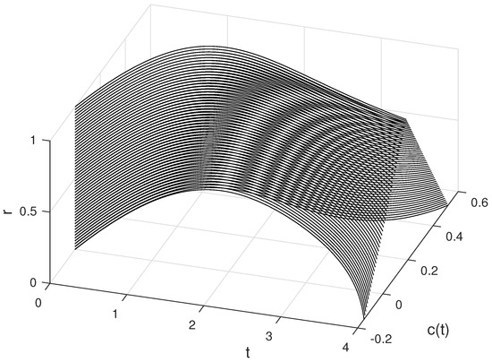
Figure 1. The approximate solutions of C for different values of r and $t$.

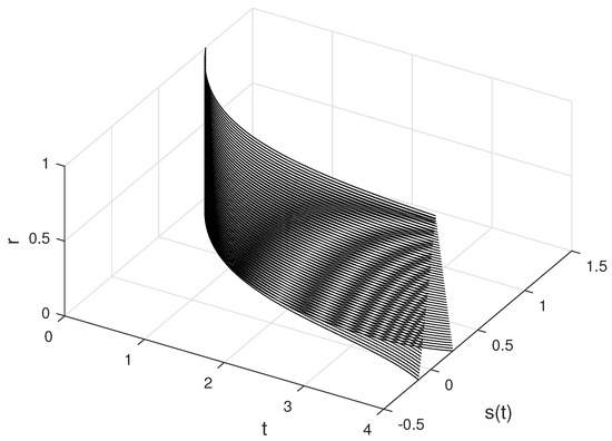
Figure 2. The approximate solutions of S for different values of r and $t$.

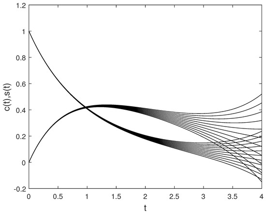
Figure 3. The approximate solutions of C and S for different values of $r=0,0.2,0.4,\dots ,1$.

Example 2.

$\lambda =4;{\eta }_0=1;{\eta }_1=0.5;\theta =3$ together with fuzzy initial values:

$$C(0;r)[{10}^{-3}(-1+r),{10}^{-3}(1-r)],$$

$$S(0;r)=[{10}^{-3}(999+r),{10}^{-3}(1001-r)].$$

In Figure 4 and Figure 5, $c(t)$ and $s(t)$ for $0\le t\le 1$ with $h_{\left[t\right]}=0.025$ are plotted, respectively. In Figure 6, $c(t)$ and $s(t)$ are plotted for different values of $r$.

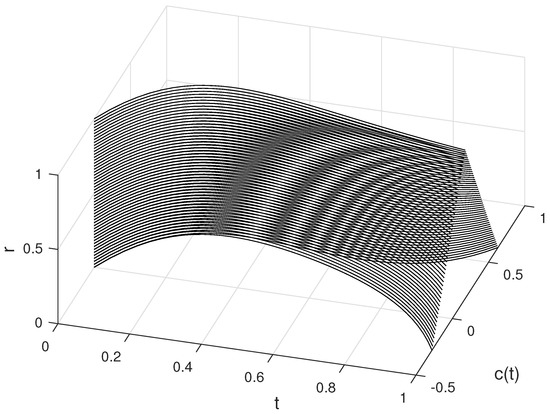
Figure 4. The approximate solutions of C for different values of r and $t$.

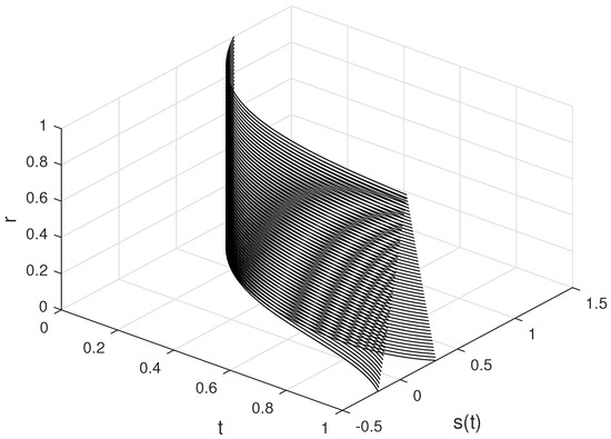
Figure 5. The approximate solutions of S for different values of r and $t$.

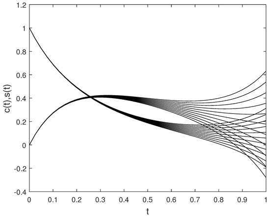
Figure 6. The approximate solutions of C and S for different values of $r=0,0.2,0.4,\dots ,1$.

Example 3.

$\lambda =20;{\eta }_0=1;{\eta }_1=1;\theta =12$ together with fuzzy initial values:

$$C(0;r)=[{10}^{-3}(-1+r),{10}^{-3}(1-r)],$$

$$S(0;r)=[9.9+0.1r,10.1-0.1r].$$

In Figure 7 and Figure 8, $c(t)$ and $s(t)$ for $0\le t\le 0.1$ with $h_{\left[t\right]}=0.0025$ are plotted, respectively. In Figure 9, $c(t)$ and $s(t)$ are plotted for different values of $r$.

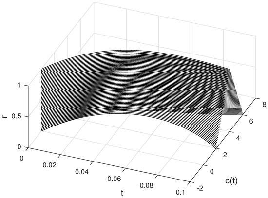
Figure 7. The approximate solutions of C for different values of r and $t$.

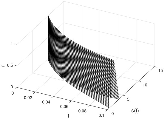
Figure 8. The approximate solutions of S for different values of r and $t$.

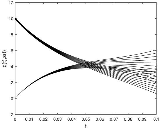
Figure 9. The approximate solutions of C and S for different values of $r=0,0.2,0.4,\dots ,1$.

In Figure 1, Figure 2, Figure 4, Figure 5, Figure 7 and Figure 8, the approximate fuzzy values obtained by the fuzzy fourth order Runge–Kutta method are presented for different values of parameters, which shows us that they are all fuzzy numbers. In Figure 3, Figure 6 and Figure 9, the speed of reaching the equilibrium point is shown by increasing the concentration, which corresponds to the real-world enzyme reactions.

7. Conclusions

In this paper, we introduced the fuzzy fourth order Runge–Kutta method for approximate solutions of the fuzzy enzyme kinetic reaction equations and illustrated it by numerical examples. Since the Runge–Kutta method has a high convergence order, it can provide appropriate approximate solutions to solve fuzzy enzyme kinetics equations. The presented examples show that the speed of reaching the equilibrium point is shown by increasing the concentration, which corresponds to the real-world enzyme reactions and confirms the suitability of the mentioned method. The algorithm presented here can easily be used for this type of fuzzy system.

References

- Kirk, O.; Borchert, T.V.; Fuglasang, C.C. Industrial enzyme applications. Curr. Opin. Biotechnol. 2002, 13, 345–351. [Google Scholar] [CrossRef]
- Buxbaum, E. Fundamentals of Protein Structure and Function, 2nd ed.; Springer International Publishing: New York, NY, USA, 2015. [Google Scholar]
- Keener, J.; Sneyd, J. Mathematical Physiology; Springer: New York, NY, USA, 1978. [Google Scholar]
- Berg, J.M.; Tymoczko, J.L.; Stryer, L. Biochemistry, 5th ed.; W. H. Freeman: San Francisco, CA, USA, 2002. [Google Scholar]
- Chasnov, J.R. Mathematical Biology Lecture notes for MATH 365; The Hong Kong University of Science and Technology: Hongkong, China, 2009. [Google Scholar]
- Chapwanya, M.; Lubuma, J.M.; Mickens, R.E. From enzyme kinetics to epidemiological models with Michaelis–Menten contact rate: Design of nonstandard finite difference schemes. Comput. Math. Appl. 2012, 64, 201–213. [Google Scholar] [CrossRef]
- Sen, A.K. An Application of the Adomian decomposition method to the transient behaviour of a model biochemical reaction. J. Math. Anal. Appl. 1988, 131, 232–245. [Google Scholar] [CrossRef]
- Khader, M.M. On the numerical solutions to nonlinear biochemical reaction model using Picard-Pade technique. World J. Model. Simul. 2013, 9, 38–46. [Google Scholar]
- Batiha, A.M.; Batiha, B. Differential Transformation Method for a Reliable Treatment of the Nonlinear Biochemical Reaction Model. Adv. Stud. Biol. 2011, 3, 355–360. [Google Scholar]
- Zadeh, L.A. Fuzzy sets. Inf. Control 1965, 8, 338–353. [Google Scholar] [CrossRef]
- Chang, S.L.; Zadeh, L.A. On fuzzy mapping and control. IEEE Trans. Syst. Man Cybern. 1972, 2, 30–34. [Google Scholar] [CrossRef]
- Dubois, D.; Prade, H. Toward fuzzy differential calculus: Part 3, differentiation. Fuzzy Sets Syst. 1982, 8, 225–233. [Google Scholar] [CrossRef]
- Seikkala, S. On the fuzzy initial value problem. Fuzzy Sets Syst. 1987, 24, 319–330. [Google Scholar] [CrossRef]
- Kaleva, O. Fuzzy differential equations. Fuzzy Sets Syst. 1987, 24, 301–317. [Google Scholar] [CrossRef]
- Kaleva, O. The Cauchy problem for fuzzy differential equations. Fuzzy Sets Syst. 1990, 35, 389–396. [Google Scholar] [CrossRef]
- Buckley, J.J.; Feuring, T. Fuzzy differential equations. Fuzzy Sets Syst. 2000, 110, 43–54. [Google Scholar] [CrossRef]
- Goetschel, R.; Voxman, W. Elementary calculus. Fuzzy Sets Syst. 1986, 18, 31–43. [Google Scholar] [CrossRef]
- Ma, M.; Friedman, M.; Kandel, A. Numerical solution of fuzzy differential equations. Fuzzy Sets Syst. 1999, 105, 133–138. [Google Scholar] [CrossRef]
- Puri, M.L.; Ralescu, D. Differential for fuzzy function. J. Math. Anal. Appl. 1983, 91, 552–558. [Google Scholar] [CrossRef]
- Nieto, J.J. The Cauchy problem for continuous fuzzy differential equations. Fuzzy Sets Syst. 1999, 102, 259–262. [Google Scholar] [CrossRef]
- Stefanini, L.; Bede, B. Generalized fuzzy differentiability with LU-parametric reperesentation. Fuzzy Sets Syst. 2014, 257, 184–203. [Google Scholar] [CrossRef]
- Abbasbandy, S.; Allahviranloo, T. Numerical solution of fuzzy differential equation by Runge–Kutta method. Nonlinear Stud. 2004, 11, 117–129. [Google Scholar] [CrossRef]
- Abbasbandy, S.; Allahviranloo, T.; Darabi, P. Numerical solution of n-order fuzzy differential equation by Runge–Kutta method. Math. Comput. Appl. 2011, 16, 935–946. [Google Scholar] [CrossRef]
- Palligkinis, S.C.; Papageorgiou, G.; Famelis, I.T. Runge–Kutta methods for fuzzy differential equations. Appl. Math. Comput. 2009, 209, 97–105. [Google Scholar] [CrossRef]
- Gomes, L.T.; de Barros, L.C.L.; Bede, B. Fuzzy Differentiatial Equations in Various Approaches; Springer: New York, NY, USA, 2015. [Google Scholar]
- Ralston, A.; Rabinowitz, P. First Course in Numerical Analysis, 2nd ed.; Dover Publications: New York, NY, USA, 2001. [Google Scholar]
- Bede, B.; Rudas, I.J.; Bencsik, A.L. First order linear fuzzy differential equations under generalized differentiability. Inf. Sci. 2007, 177, 1648–1662. [Google Scholar] [CrossRef]
- Chalco-Cano, Y.; Roman-Flores, H. On new solutions of fuzzy differential equations. Chaos Solitons Fractals 2008, 38, 112–119. [Google Scholar] [CrossRef]
- Gear, C.W. Numerical Initial Value Problem in Ordinary Differential Equations; Prentice Hall: Englewood Cliffs, NJ, USA, 1971. [Google Scholar]
© 2018 by the authors. Licensee MDPI, Basel, Switzerland. This article is an open access article distributed under the terms and conditions of the Creative Commons Attribution (CC BY) license (http://creativecommons.org/licenses/by/4.0/).