On Existence and Uniqueness of Solutions to the Fuzzy Dynamic Equations on Time Scales

Abstract

In this paper, we introduce a new metric on the space of fuzzy continuous functions on time scales by using the exponential function, $e_{\mathsf{\gamma }}(t,t_0)$, where $\mathsf{\gamma }>0$ is a constant. Then, we provide some conditions to prove an existence and uniqueness theorem for solutions to nonlinear fuzzy dynamic equations. Furthermore, we present three different examples including a practical example to illustrate the main results.

1. Introduction

Mathematical modeling of some phenomena becomes more realistic and suitable by non-continuous dynamical equations, so, in this regard, it is necessary to consider both continuous and discrete models for such problems. These equations can be interpreted by idea time scales, which was introduced for the first time in 1988 by Stefan Hilger [1] (for more details please see [2]). The time scales calculus is a unification of the continuous and discrete analysis, which describes the difference and differential equations together as well as allowing us to deal with combining equations of two differential and difference equations simultaneously (see, for example, [2,3,4,5]).

The theory of dynamic equations on time scales has many interesting applications in control theory, mathematical economics, mathematical biology, engineering and technology (see [2,6,7,8,9]). In some cases, there exists uncertainty, ambiguity or vague factors in such problems, and fuzzy theory and interval analysis are powerful tools for modeling these equations on time scales. In [10], authors introduced and considered the notions of delta derivative and delta integral to fuzzy valued functions on time scales. These definitions may accurately describe fuzzy dynamic processes where time may flow continuously and discretely at different stages in the one model; in other words, these concepts are useful in modelling fuzzy start–stop processes.

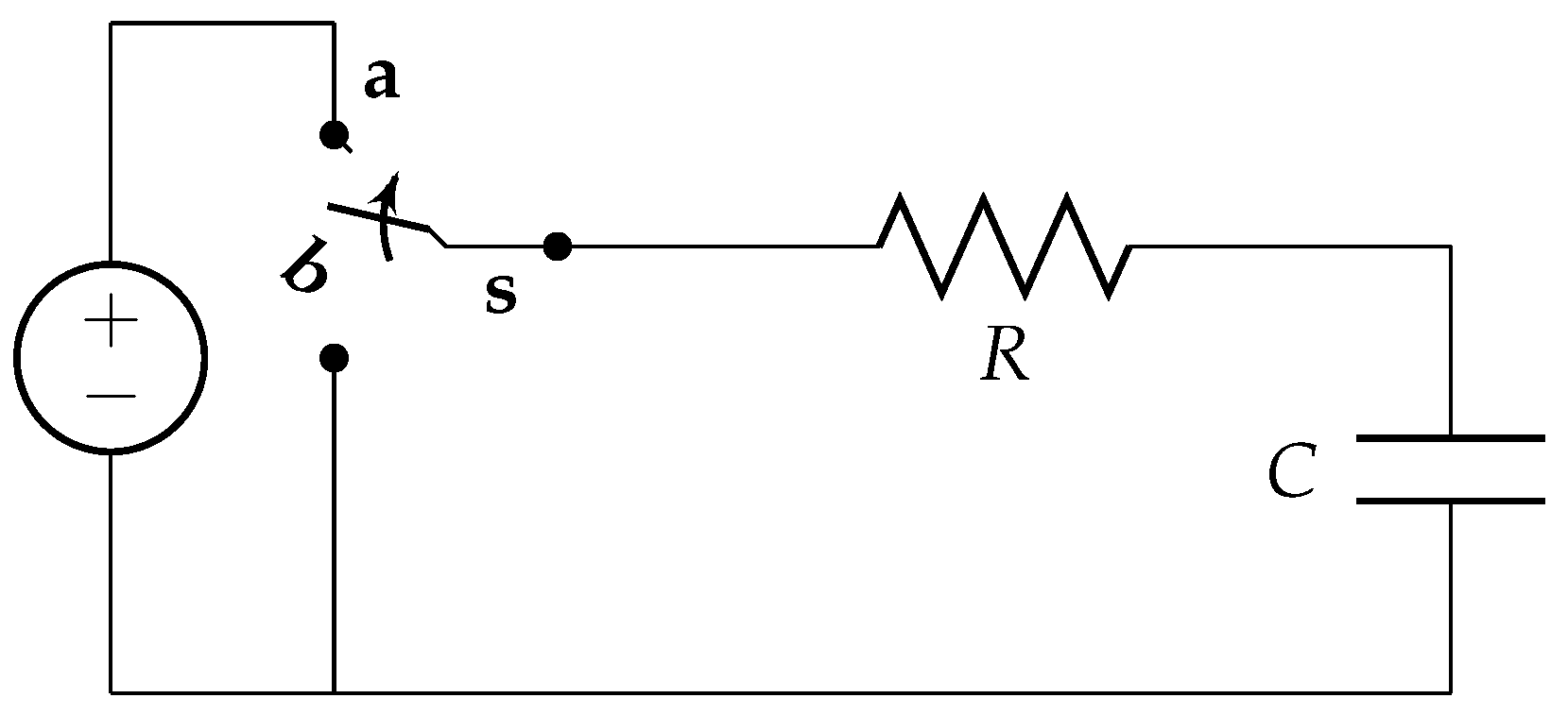
As an application, consider an electric circuit of resistor R, with unit Ω, in a series with capacitance C farads and a generator of V volts.

Note that, in an electrical $RC$ circuit when switch $\mathbf{s}$ is closed on $\mathbf{a}$, the capacitor is charged through the resistor and when the switch is afterward closed on $\mathbf{b}$, the capacitor discharges through the resistor. Suppose we discharge the capacitor periodically every time unit and assume that the discharging takes $\mathsf{\delta }>0$ but is small on time units. Thus, we can simulate it by using the time scales $P={\bigcup }_{k\in {\mathbb{N}}_0}[k,k+1-\mathsf{\delta }]$. Now, according to the assumptions of the problem, we have

$$V\left(t\right)=R{q}_t^{\mathsf{\delta }}+{\displaystyle \frac{q}{C}}$$

(1)

The dynamic Equation (1) describes the time variation of the charge q on the capacitor Figure 1 and t is in a time scale and $q_t^{\mathsf{\delta }}$ is a delta derivative of q with respect to t. Then, the problem along with a fuzzy initial condition is a first order fuzzy dynamic equation on the time scale P.

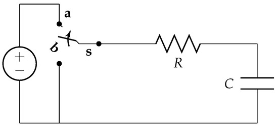
Figure 1. The capacitor described by dynamic Equation (1). Here, R is the resistor, C is capacitor, $\mathbf{s}$ is the switch, $\mathbf{a}$ and $\mathbf{b}$ are points for charging and discharging, respectively.

Recently, the theory of fuzzy difference equations in [11] and a theory of fuzzy differential equations [12,13,14] has been studied separately. In the current work, we are going to incorporate these two theories and describe a new fuzzy theory that is called the theory of fuzzy dynamic equations on time scales, and it is a generalization of the theory of fuzzy differentials and fuzzy difference equations.

To this end, we aim to study the existence and uniqueness of solutions to fuzzy dynamic equations on time scales with a new metric on fuzzy continuous functions on time scales, which is defined in terms of the exponential functions on time scales. This metric greatly simplifies the application of Banach’s theorem for the existence and uniqueness proofs. Indeed, a significant interest of this work is to utilize the rich qualities of the exponential functions on time scales. In fact, the first metric in terms of the exponential functions on time scales is introduced by Tisdell and its colleague [15], and we generalized it from crisp case to fuzzy case.

This paper is organized as follows. In Section 2, notions of the theory of fuzzy and time scales are introduced. Then, the fuzzy delta derivative and delta integral are defined in Section 3. In addition, a new metric on the space of fuzzy continuous functions on time scales is introduced. Finally, in the last section, the existence and uniqueness of the solution to a nonlinear fuzzy dynamic equations on time scales is established.

2. Preliminaries

For a better understanding, the notations used throughout the paper and keeping the paper somewhat self-contained, this section contains some preliminary definitions and associated notations.

Definition 1.

Let X be a nonempty set. A fuzzy set u in X is characterized by its membership function $u:X\to [0,1]$. Then, $u\left(x\right)$ is interpreted as the degree of membership of an element x in the fuzzy set u for each $x\in X$ [16].

Let us denote by ${\mathbb{R}}_{\mathcal{F}}$ the class of fuzzy subsets of the real axis (i.e., $u:\mathbb{R}\to [0,1]$), satisfying the following properties:

• u is normal, i.e., there exists $x_0\in \mathbb{R}$ with $u\left(x_0\right)=1$,
• u is a fuzzy-convex set (i.e., $u(tx+(1-t\left)y\right)\ge min\left\{u\right(x),u(y\left)\right\},\forall t\in [0,1],x,y\in \mathbb{R})$,
• u is upper semicontinuous on $\mathbb{R}$,
• $cl\{x\in \mathbb{R};u(x)>0\}$ is compact, where $cl$ denotes the closure of a subset.

Then, ${\mathbb{R}}_{\mathcal{F}}$ is called the space of fuzzy numbers. Obviously, $\mathbb{R}\subset {\mathbb{R}}_{\mathcal{F}}$. Here, $\mathbb{R}\subset {\mathbb{R}}_{\mathcal{F}}$ is understood as $\mathbb{R}=\{{\chi }_{\left\{x\right\}};x\mathrm{is}\mathrm{a}\mathrm{usual}\mathrm{real}\mathrm{number}\}$. For $0<\mathsf{\alpha }\le 1$, denote ${\left[u\right]}^{\mathsf{\alpha }}=\{x\in \mathbb{R};u\left(x\right)\ge \mathsf{\alpha }\}$ and ${\left[u\right]}^0=cl\{x\in \mathbb{R};u\left(x\right)>0\}$.

Using the definition of fuzzy numbers, it follows that, for any $\mathsf{\alpha }\in [0,1]$, ${\left[u\right]}^{\mathsf{\alpha }}$ is a bounded closed interval. The notation ${\left[u\right]}^{\mathsf{\alpha }}=[{\underline{u}}^{\mathsf{\alpha }},{\overline{u}}^{\mathsf{\alpha }}]$ denotes explicitly the $\mathsf{\alpha }$-level set of u. We refer to $\underline{u}$ and $\overline{u}$ as the lower and upper branches on u, respectively.

For $u,v\in {\mathbb{R}}_{\mathcal{F}}$ and $\mathsf{\lambda }\in \mathbb{R}$, the sum $u+v$ and the product $\mathsf{\lambda }·u$ are defined by ${[u+v]}^{\mathsf{\alpha }}={\left[u\right]}^{\mathsf{\alpha }}+{\left[v\right]}^{\mathsf{\alpha }}$, ${[\mathsf{\lambda }·u]}^{\mathsf{\alpha }}=\mathsf{\lambda }{\left[u\right]}^{\mathsf{\alpha }}$, $\forall \mathsf{\alpha }\in [0,1]$, where ${\left[u\right]}^{\mathsf{\alpha }}+{\left[v\right]}^{\mathsf{\alpha }}=\{x+y:x\in {\left[u\right]}^{\mathsf{\alpha }},y\in {\left[v\right]}^{\mathsf{\alpha }}\}$ means the usual addition of two intervals of $\mathbb{R}$ and $\mathsf{\lambda }{\left[u\right]}^{\mathsf{\alpha }}=\{\mathsf{\lambda }·x:x\in {\left[u\right]}^{\mathsf{\alpha }}\}$ means the usual product between a scalar and a subset of $\mathbb{R}$.

Theorem 1.

According to Bede et al. [13].

• If we denote $\tilde{0}={\chi }_{\left\{0\right\}},$ then $\tilde{0}\in {\mathbb{R}}_{\mathcal{F}}$ is the zero element with respect to +, i.e., $u+\tilde{0}=\tilde{0}+u=u$ , for all $u\in {\mathbb{R}}_{\mathcal{F}}$.
• For any $a,b\in \mathbb{R}$ with $a,b\le 0$ or $a,b\ge 0$ and any $u\in {\mathbb{R}}_{\mathcal{F}}$, we have $(a+b)·u=a·u+b·u$; for general $a,b\in \mathbb{R}$, the above property does not hold.
• For any $\mathsf{\lambda }\in \mathbb{R}$ and any $u,v\in {\mathbb{R}}_{\mathcal{F}}$, we have $\mathsf{\lambda }·(u+v)=\mathsf{\lambda }·u+\mathsf{\lambda }·v$.
• For any $\mathsf{\lambda },\mathsf{\mu }\in \mathbb{R}$ and any $u\in {\mathbb{R}}_{\mathcal{F}}$, we have $\mathsf{\lambda }·(\mathsf{\mu }·u)=\left(\mathsf{\lambda }\mathsf{\mu }\right)·u$.

Definition 2.

Let $x,y\in {\mathbb{R}}_{\mathcal{F}}$. If there exists $z\in {\mathbb{R}}_{\mathcal{F}}$ such that $x=y+z$, then z is called the H-difference of x and y, and it is denoted by $x\ominus y$ [13].

Let $D:{\mathbb{R}}_{\mathcal{F}}\times {\mathbb{R}}_{\mathcal{F}}\to {\mathbb{R}}^{+}\cup \left\{0\right\}$, $D(u,v)={sup}_{\mathsf{\alpha }\in [0,1]}max\left\{\right|{\underline{u}}^{\mathsf{\alpha }}-{\underline{v}}^{\mathsf{\alpha }}|,|{\overline{u}}^{\mathsf{\alpha }}-{\overline{v}}^{\mathsf{\alpha }}\left|\right\}$ be the Hausdorff distance between fuzzy numbers, where ${\left[u\right]}^{\mathsf{\alpha }}=[{\underline{u}}^{\mathsf{\alpha }},{\overline{u}}^{\mathsf{\alpha }}]$, ${\left[v\right]}^{\mathsf{\alpha }}=[{\underline{v}}^{\mathsf{\alpha }},{\overline{v}}^{\mathsf{\alpha }}]$. The following properties are well-known (see [12,13]):

• $D(u+w,v+w)=D(u,v),\forall u,v,w\in {\mathbb{R}}_{\mathcal{F}}$,
• $D(k·u,k·v)=\left|k\right|D(u,v),\forall k\in \mathbb{R}$, $u,v\in {\mathbb{R}}_{\mathcal{F}},$
• $D(u+v,w+e)\le D(u,w)+D(v,e),\forall u,v,w,e\in {\mathbb{R}}_{\mathcal{F}}$,
• $D(u\ominus v,e\ominus w)\le D(u,e)+D(v,w),$

where $({\mathbb{R}}_{\mathcal{F}},D)$ is a complete metric space. In addition, we define for each $x,y\in C(I,{\mathbb{R}}_{\mathcal{F}})$, $D(x,y)={sup}_{t\in I}D(x\left(t\right),y\left(t\right))$, which $C(I,{\mathbb{R}}_{\mathcal{F}})$ is a set of all fuzzy continuous functions on I.

Definition 3.

Given $u,v\in {\mathbb{R}}_{\mathcal{F}}$, the $gH$-difference is the fuzzy number w, if it exists, such that

$$u{\ominus }_{gH}v=w\iff \left\{\begin{array}{c}\left(i\right)u=v+w,\hfill \\ or\left(ii\right)v=u+(-1)·w.\hfill \end{array}\right.$$

(2)

If $u{\ominus }_{gH}v$ exists, its $\mathsf{\alpha }$ cuts are given by

$${\left[u{\ominus }_{gH}v\right]}^{\mathsf{\alpha }}=[min\{{\underline{u}}^{\mathsf{\alpha }}-{\underline{v}}^{\mathsf{\alpha }},{\overline{u}}^{\mathsf{\alpha }}-{\overline{v}}^{\mathsf{\alpha }}\},max\{{\underline{u}}^{\mathsf{\alpha }}-{\underline{v}}^{\mathsf{\alpha }},{\overline{u}}^{\mathsf{\alpha }}-{\overline{v}}^{\mathsf{\alpha }}\}]$$

and $u\ominus v=u{\ominus }_{gH}v$ if $u\ominus v$ exists. If $\left(i\right)$ and $\left(ii\right)$ are satisfied simultaneously, then w is a crisp number [17,18].

Remark 1.

In the fuzzy case, it is possible that the $gH$-difference of two fuzzy numbers does not exist. If $u{\ominus }_{gH}v$ exists, then $v{\ominus }_{gH}u$ exists and $v{\ominus }_{gH}u=-\left(u{\ominus }_{gH}v\right)$. The following properties have been obtained in [17,18].

Proposition 1.

Let $u,v\in {\mathbb{R}}_{\mathcal{F}}$ be two fuzzy numbers [17,18] ; then,

• if the $gH$-difference exists, it is unique;
• $u{\ominus }_{gH}v=u\ominus v$ or $u{\ominus }_{gH}v=-(u\ominus v)$ whenever the expressions on the right exist; in particular, $u{\ominus }_{gH}u=u\ominus u=\tilde{0}$;
• if $u{\ominus }_{gH}v$ exists in the sense (i), then $v{\ominus }_{gH}u$ exists in the sense (ii) and vice versa;
• $(u+v){\ominus }_{gH}v=u$;
• $\tilde{0}{\ominus }_{gH}\left(u{\ominus }_{gH}v\right)=v{\ominus }_{gH}u$;
• $u{\ominus }_{gH}v=v{\ominus }_{gH}u=w$ if and only if $w=-w$; furthermore, $w=\tilde{0}$ if and only if $u=v$.

Definition 4.

A time scale $\mathbb{T}$ is a non-empty, closed subset of $\mathbb{R}$, equipped with the topology induced from the standard topology on $\mathbb{R}$ [2].

According to Definition 4, a time scale can be continuous and discrete or continuous-discrete. Hence, the definition of jump operator is very important to time scales.

Definition 5.

The forward (backward) jump operator $\mathsf{\sigma }\left(t\right)$ at t for $t<sup\mathbb{T}$ (respectively, $\mathsf{\rho }\left(t\right)$ at t for $t>inf\mathbb{T}$) is given by

$$\mathsf{\sigma }\left(t\right)=inf\{\mathsf{\tau }>t:\tau \in \mathbb{T}\},\left(\rho \right(t)=sup\{\mathsf{\tau }<t:\mathsf{\tau }\in \mathbb{T}\left\}\right)\mathit{for}\mathit{all}t\in \mathbb{T}.$$

(3)

Additionally, $\mathsf{\sigma }(sup\mathbb{T})=sup\mathbb{T}$, if $sup\mathbb{T}<\infty$, and $\mathsf{\rho }(inf\mathbb{T})=inf\mathbb{T}$ if $inf\mathbb{T}>-\infty$. Furthermore, the graininess function $\mathsf{\mu }:\mathbb{T}\to {\mathbb{R}}^{+}$ is defined by $\mathsf{\mu }\left(t\right)=\mathsf{\sigma }\left(t\right)-t$ and also the left-graininess function $\nu :\mathbb{T}\to {\mathbb{R}}^{+}$ is defined by $\nu \left(t\right)=t-\mathsf{\rho }\left(t\right)$ [2].

It is enough to recognize that, for connected points, the forward and backward jump operators return the same element of the time scale that was drawn from the domain. However, for non-connected points, the forward and backward jump operators return the next and previous elements of the time scale, respectively. The jump operators then enable the classification of points in a time scale in the following way:

Definition 6.

If $\mathsf{\sigma }\left(t\right)>t$, then the point t is called right-scattered; while, if $\rho \left(t\right)<t,$ then t is termed left-scattered. If $t<sup\mathbb{T}$ and $\mathsf{\sigma }\left(t\right)=t,$ then the point t is called right-dense; while if $t>inf\mathbb{T}$ and $\rho \left(t\right)=t$, then we say that t is left-dense [2].

Definition 7.

A mapping $f:\mathbb{T}\to {\mathbb{R}}_{\mathcal{F}}$ is rd-continuous if it is continuous at each right-dense point and its left-side limits exist (finite) at left-dense points in $\mathbb{T}$. We denote the set of rd-continuous functions from $\mathbb{T}$ to ${\mathbb{R}}_{\mathcal{F}}$ by $C_{rd}[\mathbb{T},{\mathbb{R}}_{\mathcal{F}}]$.

Definition 8.

Fix $t\in \mathbb{T}$ and $f:\mathbb{T}\to \mathbb{R}$. Define $f^{\mathsf{\delta }}\left(t\right)$ to be the real number (provided it exists) with the property that, given $ϵ>0$, there is a neighborhood $U_{\mathbb{T}}$ of t (i.e., $U_{\mathbb{T}}=(t-\mathsf{\delta },t+\mathsf{\delta })\cap \mathbb{T}$) such that

$$|(f\left(\mathsf{\sigma }\left(t\right)\right)-f\left(s\right))-f^{\mathsf{\delta }}\left(t\right)(\mathsf{\sigma }\left(t\right)-s)|\le ϵ|\mathsf{\sigma }\left(t\right)-s|,$$

for all $s\in U_{\mathbb{T}}$. $f^{\mathsf{\delta }}\left(t\right)$ is called the $\mathsf{\delta }$-derivative of f at t [2].

Definition 9.

We say that a function $f:\mathbb{T}\to \mathbb{R}$ is right-increasing at a point $t_0\in \mathbb{T}\backslash \{min\mathbb{T}\}$ provided that [19]:

• if $t_0$ is right-scattered, then $f\left(t_0\right)<f\left(\mathsf{\sigma }\left(t_0\right)\right);$
• if $t_0$ is right-dense, then there is a neighborhood $U_{\mathbb{T}}=(t_0-\mathsf{\delta },t_0+\mathsf{\delta })\cap \mathbb{T}$ of $t_0$ such that

  $$f\left(t\right)>f\left(t_0\right)\mathit{for}\mathit{all}t\in U_{\mathbb{T}}\mathit{with}t>t_0.$$

Similarly, we say that f is right-decreasing if in $\left(i\right)$, $f\left(\mathsf{\sigma }\left(t_0\right)\right)<f\left(t_0\right)$ and in $\left(ii\right)$, $f\left(t\right)<f\left(t_0\right)$.

Theorem 2.

Suppose $f:\mathbb{T}\to \mathbb{R}$ is differentiable at $t_0\in \mathbb{T}\backslash \{min\mathbb{T}\}$ [19]. If $f^{\mathsf{\delta }}\left(t_0\right)>0$, then f is right-increasing at the point $t_0$. If $f^{\mathsf{\delta }}\left(t_0\right)<0$, then f is right-decreasing at the point $t_0$.

Here, we review some properties of the exponential function on time scales. For more details, we refer to Definition 2.30 in [2].

A function $p:\mathbb{T}\to \mathbb{R}$ is called regressive if $1+\mathsf{\mu }\left(t\right)p\left(t\right)\ne 0$ for all $t\in \mathbb{T}$ and the function p is called positively regressive if $1+\mathsf{\mu }\left(t\right)p\left(t\right)>0$ for all $t\in \mathbb{T}$. If $p:\mathbb{T}\to \mathbb{R}$ is a regressive function and $t_0\in \mathbb{T}$, then (see Theorem 2.33 in [2]) the exponential function $e_p(.,t_0)$ is the unique solution of the initial value problem

$$y^{\mathsf{\delta }}\left(t\right)=p\left(t\right)y\left(t\right),y\left(t_0\right)=1$$

The following properties of the exponential function will be used in the last section:

• $e_0(t,s)=1$, $e_p(t,t)=1;$
• $e_p(\mathsf{\sigma }\left(t\right),s)=[1+\mathsf{\mu }\left(t\right)p\left(t\right)]e_p(t,s);$
• $e_p(t,r)e_p(r,s)=e_p(t,s);$
• $e_p(t,s)=\frac{1}{e_p(s,t)};$
• $e_p^{\mathsf{\delta }}(t,t_0)=p\left(t\right)e_p(t,t_0).$

The set ${\mathbb{T}}^k$ is defined to be $\mathbb{T}\backslash \left\{m\right\}$ if $\mathbb{T}$ has a left-scattered maximum m. Otherwise, ${\mathbb{T}}^k=\mathbb{T}$.

3. Fuzzy Delta Derivative and Integral on Time Scales

Definition 10.

Assume that $f:\mathbb{T}\to {\mathbb{R}}_{\mathcal{F}}$ is a fuzzy function and let $t\in {\mathbb{T}}^k$ [10]. Then, f is said to be right fuzzy delta differentiable at t, if there exists an element ${\mathsf{\delta }}_H^{+}f\left(t\right)$ of ${\mathbb{R}}_{\mathcal{F}}$ with the property that, given any $ϵ>0$, there exists a neighborhood $U_{\mathbb{T}}$ of t [i.e., $U_{\mathbb{T}}=(t-\mathsf{\delta },t+\mathsf{\delta })\cap \mathbb{T}$ for some $\mathsf{\delta }>0$ such that for all $t+h\in U_{\mathbb{T}}$

$$D[f(t+h){\ominus }_{gH}f\left(\mathsf{\sigma }\left(t\right)\right),{\mathsf{\delta }}_H^{+}f\left(t\right)(h-\mathsf{\mu }\left(t\right))]\le ϵ(h-\mathsf{\mu }\left(t\right)),$$

with $0\le h<\mathsf{\delta }$.

Definition 11.

Assume that $f:\mathbb{T}\to {\mathbb{R}}_{\mathcal{F}}$ is a fuzzy function and let $t\in {\mathbb{T}}^k$ [10]. Then, f is said to be left fuzzy delta differentiable at t, if there exists an element ${\mathsf{\delta }}_H^{-}f\left(t\right)$ of ${\mathbb{R}}_{\mathcal{F}}$ with the property that, given any $ϵ>0$, there exists a neighborhood $U_{\mathbb{T}}$ of t such that for all $t-h\in U_{\mathbb{T}}$

$$D[f\left(\mathsf{\sigma }\left(t\right)\right){\ominus }_{gH}f(t-h),{\mathsf{\delta }}_H^{-}f\left(t\right)(h+\mathsf{\mu }\left(t\right))]\le ϵ(h+\mathsf{\mu }\left(t\right)),$$

with $0\le h<\mathsf{\delta }$.

In the above definitions ${\mathsf{\delta }}_H^{+}f\left(t\right)$ and ${\mathsf{\delta }}_H^{-}f\left(t\right)$ are called, respectively, right fuzzy delta derivative and left fuzzy delta derivative at t.

Definition 12.

Let $f:\mathbb{T}\to {\mathbb{R}}_{\mathcal{F}}$ be a fuzzy function and $t\in {\mathbb{T}}^k$ [10]. Then, f is said to be $\mathsf{\delta }$-Hukuhara differentiable at t, if f is both left and right fuzzy delta differentiable at $t\in {\mathbb{T}}^k$ and ${\mathsf{\delta }}_H^{+}f\left(t\right)={\mathsf{\delta }}_H^{-}f\left(t\right),$ and we will denote it by ${\mathsf{\delta }}_{H}f\left(t\right)$.

We call ${\mathsf{\delta }}_{H}f\left(t\right)$ the $\mathsf{\delta }$-Hukuhara derivative of f at t. We say that f is ${\mathsf{\delta }}_H$-differentiable at t if its ${\mathsf{\delta }}_H$-derivative exists at t. Moreover, we say that f is ${\mathsf{\delta }}_H$-differentiable on ${\mathbb{T}}^k$ if its ${\mathsf{\delta }}_H$-derivative exists at each $t\in {\mathbb{T}}^k$. The fuzzy function ${\mathsf{\delta }}_{H}f:{\mathbb{T}}^k\to {\mathbb{R}}_{\mathcal{F}}$ is then called the ${\mathsf{\delta }}_H$-derivative of f on ${\mathbb{T}}^k$.

Proposition 2.

If the ${\mathsf{\delta }}_H$-derivative of f at t exists, then it is unique. Hence, the ${\mathsf{\delta }}_H$-derivative is well defined [10].

Lemma 1.

Assume that $f:\mathbb{T}\to {\mathbb{R}}_{\mathcal{F}}$ is ${\mathsf{\delta }}_H$-differentiable at $t\in {\mathbb{T}}^k$, then f is continuous at t [10].

Theorem 3.

Assume that $f:\mathbb{T}\to {\mathbb{R}}_{\mathcal{F}}$ is a function and let $t\in {\mathbb{T}}^k$, then we have the following [10]:

• If f is continuous at t and t is right-scattered, then f is ${\mathsf{\delta }}_H$-differentiable at t with

  $${\mathsf{\delta }}_{H}f\left(t\right)=\frac{f\left(\mathsf{\sigma }\left(t\right)\right){\ominus }_{gH}f\left(t\right)}{\mathsf{\mu }\left(t\right)}$$

  (4)
• If t is right-dense, then f is ${\mathsf{\delta }}_H$-differentiable at t iff the limits

  $$\underset{h\to 0^{+}}{lim}\frac{f(t+h){\ominus }_{gH}f\left(t\right)}{h}\mathit{and}\underset{h\to 0^{+}}{lim}\frac{f\left(t\right){\ominus }_{gH}f(t-h)}{h}$$

  exist and satisfy in this case

  $$\underset{h\to 0^{+}}{lim}\frac{f(t+h){\ominus }_{gH}f\left(t\right)}{h}=\underset{h\to 0^{+}}{lim}\frac{f\left(t\right){\ominus }_{gH}f(t-h)}{h}={\mathsf{\delta }}_{H}f\left(t\right)$$

  (5)

Lemma 2.

If f is ${\mathsf{\delta }}_H$-differentiable at $t\in {\mathbb{T}}^k$, then $f\left(\mathsf{\sigma }\left(t\right)\right)=f\left(t\right)+\mathsf{\mu }\left(t\right){\mathsf{\delta }}_{H}f\left(t\right)$ or $f\left(t\right)=f\left(\mathsf{\sigma }\left(t\right)\right)+(-1)\mathsf{\mu }\left(t\right){\mathsf{\delta }}_{H}f\left(t\right)$ [10].

Remark 2.

Assuming that f is ${\mathsf{\delta }}_H$-differentiable, we say that f is ${\mathsf{\delta }}_H$-differentiable in the sense $\left(i\right)$ or $\left(i\right){\mathsf{\delta }}_H$-differentiable if, in the definition of ${\mathsf{\delta }}_H$-derivative, the $gH$-difference is equivalent to the H-difference and we say that f is ${\mathsf{\delta }}_H$-differentiable in the sense $\left(ii\right)$ or $\left(ii\right){\mathsf{\delta }}_H$-differentiable if $gH$-difference is equivalent to another case.

Lemma 3.

If $f,g:\mathbb{T}\to {\mathbb{R}}_{\mathcal{F}}$ are ${\mathsf{\delta }}_H$-differentiable at $t\in {\mathbb{T}}^k$, in the same case of ${\mathsf{\delta }}_H$-differentiability (both are $\left(i\right){\mathsf{\delta }}_H$-differentiable or $\left(ii\right){\mathsf{\delta }}_H$-differentiable), then $f+g:\mathbb{T}\to {\mathbb{R}}_{\mathcal{F}}$ is also ${\mathsf{\delta }}_H$-differentiable at t and

$${\mathsf{\delta }}_H(f+g)\left(t\right)={\mathsf{\delta }}_{H}f\left(t\right)+{\mathsf{\delta }}_{H}g\left(t\right)$$

(6)

Proof. 

It can be easily proved by using Theorem 3. ☐

Lemma 4.

If $f:\mathbb{T}\to {\mathbb{R}}_{\mathcal{F}}$ is ${\mathsf{\delta }}_H$-differentiable at $t\in {\mathbb{T}}^k$, then, for any nonnegative constant $\mathsf{\lambda }\in \mathbb{R}$, $\mathsf{\lambda }f:\mathbb{T}\to {\mathbb{R}}_{\mathcal{F}}$ is ${\mathsf{\delta }}_H$-differentiable at t with

$${\mathsf{\delta }}_H\left(\mathsf{\lambda }f\right)\left(t\right)=\mathsf{\lambda }{\mathsf{\delta }}_{H}f\left(t\right)$$

Proof. 

It follows easily from the Theorem 3. ☐

Now, we present the definition of integral on time scales and give some properties of integrals on time scales for fuzzy valued functions. Let $\mathbb{T}$ be a time scale, $a<b$ be points in $\mathbb{T}$, and ${[a,b]}_{\mathbb{T}}$ be the closed (and bounded) interval in $\mathbb{T}$. A partition of ${[a,b]}_{\mathbb{T}}$ is any finite ordered subset

$$P=\{t_0,t_1,\dots ,t_n\}\subset {[a,b]}_{\mathbb{T}},\mathrm{where}a=t_0<t_1<\dots <t_n=b$$

The number n depends on the particular partition, so we have $n=n\left(P\right)$. The intervals $[t_{i-1},t_i)$ for $1\le i\le n$ are called the subintervals of the partition P. We denote the set of all partitions of ${[a,b]}_{\mathbb{T}}$ by $\mathcal{P}=\mathcal{P}(a,b)$.

Lemma 5.

According to Guseinov and Kaymaklan [20], for each $\mathsf{\delta }>0$, there exists a partition $P\in \mathcal{P}(a,b)$ given by $a=t_0<t_1<\dots <t_n=b$ such that, for each $i\in \{1,2,\dots ,n\}$, either

$$t_i-t_{i-1}<\mathsf{\delta }$$

or

$$t_i-t_{i-1}>\mathsf{\delta }and\mathsf{\rho }\left(t_i\right)=t_{i-1}.$$

Definition 13.

A function $f:{[a,b]}_{\mathbb{T}}\to {\mathbb{R}}_{\mathcal{F}}$ is called Riemann $\mathsf{\delta }$-integrable on ${[a,b]}_{\mathbb{T}}$, if there exists $I_R\in {\mathbb{R}}_{\mathcal{F}}$, with the property [10]: $\forall ϵ>0,\exists \mathsf{\delta }>0$, such that for any division of ${[a,b]}_{\mathbb{T}}$, $d:a=x_0<\dots <x_n=b$ with $x_i\in {[a,b]}_{\mathbb{T}}$, and for any points ${\xi }_i\in {[x_i,x_{i+1})}_{\mathbb{T}}$, $\overline{i=0,n-1}$, we have

$$D\left[{\displaystyle \sum _{i=0}^{n-1}f\left({\xi }_i\right).(x_{i+1}-x_i),I_R}\right]<ϵ$$

Then, we denote $I_R={\int }_a^{b}f\left(x\right)\mathsf{\delta }x$ the fuzzy Riemann $\mathsf{\delta }$-integral.

Definition 14.

Let $f:{[0,t]}_{\mathbb{T}}\to {\mathbb{R}}_{\mathcal{F}}$ [10]. We define levelwise the $\mathsf{\delta }$-integral of f in ${[0,t]}_{\mathbb{T}}$, (denoted by ${\int }_{{[0,t]}_{\mathbb{T}}}f\left(t\right)\mathsf{\delta }t$ or ${\int }_0^{t}f\left(t\right)\mathsf{\delta }t$) as the set of the integrals of the measurable selections for ${\left[f\right]}^{\mathsf{\alpha }}$, for each $\mathsf{\alpha }\in (0,1]$. We say that f is $\mathsf{\delta }$-integrable over ${[0,t]}_{\mathbb{T}}$ if ${\int }_{{[0,t]}_{\mathbb{T}}}f\left(t\right)\mathsf{\delta }t\in {\mathbb{R}}_{\mathcal{F}}$ and we have

$${[{\int }_0^{t}f\left(t\right)\mathsf{\delta }t]}^{\mathsf{\alpha }}=[{\int }_0^t{\underline{f}}^{\mathsf{\alpha }}\left(t\right)\mathsf{\delta }t,{\int }_0^t{\overline{f}}^{\mathsf{\alpha }}\left(t\right)\mathsf{\delta }t]$$

(7)

for each $\mathsf{\alpha }\in (0,1]$.

Theorem 4.

If $f,g:{[a,b]}_{\mathbb{T}}\to {\mathbb{R}}_{\mathcal{F}}$ are $\mathsf{\delta }$-integrable on ${[a,b]}_{\mathbb{T}}$, then $\mathsf{\alpha }f+\beta g$, where $\mathsf{\alpha },\beta \in \mathbb{R}$, is $\mathsf{\delta }$-integrable on ${[a,b]}_{\mathbb{T}}$ and

$${\int }_a^b(\mathsf{\alpha }f\left(t\right)+\beta g\left(t\right))\mathsf{\delta }t=\mathsf{\alpha }\left({\int }_a^{b}f\left(t\right)\mathsf{\delta }t\right)+\beta \left({\int }_a^{b}g\left(t\right)\mathsf{\delta }t\right)$$

(8)

Proof. 

It easily follows from Definition 13. ☐

Theorem 5.

If $f:{[a,b]}_{\mathbb{T}}\to {\mathbb{R}}_{\mathcal{F}}$ is ${\mathsf{\delta }}_H$-differentiable on ${[a,b]}_{\mathbb{T}}$ and $a\in \mathbb{T}$, then ${\mathsf{\delta }}_{H}f\left(t\right)$ is $\mathsf{\delta }$-integrable over ${[a,b]}_{\mathbb{T}}$ and

$$f\left(s\right)=f\left(a\right)+{\int }_a^s{\mathsf{\delta }}_{H}f\left(t\right)\mathsf{\delta }t$$

or

$$f\left(a\right)=f\left(s\right)+(-1){\int }_a^s{\mathsf{\delta }}_{H}f\left(t\right)\mathsf{\delta }t$$

for any $s\in {[a,b]}_{\mathbb{T}}$.

Proof. 

By setting the functions ${\mathsf{\delta }}_L$ and ${\mathsf{\delta }}_R$ defined in Definition 15 [10] as the same constant functions, the proof immediately follows from Theorem 18 [10]. ☐

Theorem 6.

Let $f:\mathbb{T}\to {\mathbb{R}}_{\mathcal{F}}$ and let $t\in \mathbb{T}$. Then, f is $\mathsf{\delta }$-integrable from t to $\mathsf{\sigma }\left(t\right)$ and

$${\int }_t^{\mathsf{\sigma }\left(t\right)}f\left(s\right)\mathsf{\delta }s=\mathsf{\mu }\left(t\right)f\left(t\right)$$

(9)

4. New Metric Space

Now, we are ready to define a new metric for the fuzzy continuous functions on time scales.

Definition 15.

Let D denote the Hausdorff metric on space ${\mathbb{R}}_{\mathcal{F}}$. Let $\mathsf{\gamma }>0$ be a constant. We define the space of all fuzzy continuous functions on time scales, $C({[t_0,t_0+a]}_{\mathbb{T}};{\mathbb{R}}_{\mathcal{F}})$, along with $\mathsf{\gamma }$-metric, $d_{\mathsf{\gamma }}(x,y)$, which is defined by

$$d_{\mathsf{\gamma }}(x,y):=\underset{t\in {[t_0,t_0+a]}_{\mathbb{T}}}{sup}{\displaystyle \frac{D\left(x\right(t),y(t\left)\right)}{e_{\mathsf{\gamma }}(t,t_0)}}$$

(10)

for all $t\in {[t_0,t_0+a]}_{\mathbb{T}}$ and $x,y\in C({[t_0,t_0+a]}_{\mathbb{T}};{\mathbb{R}}_{\mathcal{F}}).$

In addition, since $e_0(t,s)\equiv 1$, $d_0$ is defined as

$$d_0(x,y):=\underset{t\in {[t_0,t_0+a]}_{\mathbb{T}}}{sup}D(x\left(t\right),y\left(t\right))$$

(11)

for all $t\in {[t_0,t_0+a]}_{\mathbb{T}}$ and $x,y\in C({[t_0,t_0+a]}_{\mathbb{T}};{\mathbb{R}}_{\mathcal{F}})$, which is the same as the Hausdorff metric on the fuzzy continuous functions space.

In addition, we consider

$${\parallel x\parallel }_{\mathsf{\gamma }}:=\underset{t\in {[t_0,t_0+a]}_{\mathbb{T}}}{sup}{\displaystyle \frac{D(x(t),\tilde{0})}{e_{\mathsf{\gamma }}(t,t_0)}}$$

for all $t\in {[t_0,t_0+a]}_{\mathbb{T}}$ and $x\in C({[t_0,t_0+a]}_{\mathbb{T}};{\mathbb{R}}_{\mathcal{F}})$ and ${\parallel x\parallel }_0$ is defined as

$${\parallel x\parallel }_0:=\underset{t\in {[t_0,t_0+a]}_{\mathbb{T}}}{sup}D(x\left(t\right),\tilde{0})$$

Here, $d_{\mathsf{\gamma }}$ mapping is a new generalization of the Bielecki’s metric in [21]. The following two lemmas describe some important properties of $d_{\mathsf{\gamma }}$ and ${\parallel .\parallel }_{\mathsf{\gamma }}.$

Lemma 6.

If $\mathsf{\gamma }>0$ is constant, then:

• $d_{\mathsf{\gamma }}$ is a metric and is equivalent to the sup-metric $d_0$,
• $(C{[t_0,t_0+a]}_{\mathbb{T}};{\mathbb{R}}_{\mathcal{F}}),d_{\mathsf{\gamma }})$ is a complete metric space.

Proof. 

We note that $\mathsf{\gamma }\in C_{rd}({[t_0,t_0+a]}_{\mathbb{T}};{\mathbb{R}}_{\mathcal{F}})$ as any constant function is always $rd$-continuous. Since $\mathsf{\mu }\left(t\right)\ge 0$, we have $1+\mathsf{\mu }\left(t\right)\mathsf{\gamma }>0$ for all $t\in {[t_0,t_0+a]}_{\mathbb{T}}$. Hence, $\mathsf{\gamma }\in R^{+}$ (set of positively regressive functions) and $e_{\mathsf{\gamma }}(t,t_0)>0$ for all $t\in {[t_0,t_0+a]}_{\mathbb{T}}$ (see [2]). It follows that, for each $x,y\in C({[t_0,t_0+a]}_{\mathbb{T}};{\mathbb{R}}_{\mathcal{F}}),$ we have

• since $\mathsf{\gamma }>0$, $e_{\mathsf{\gamma }}(t,t_0)>0,$ thus $d_{\mathsf{\gamma }}\ge 0$. $d_{\mathsf{\gamma }}(x,y)=0$ if and only if $D(x,y)=0$, and we know that $D(x,y)=0$ if and only if $x=y$. Since D is a metric, $d_{\mathsf{\gamma }}(x,y)=d_{\mathsf{\gamma }}(y,x)$. In addition, we have

  $$\begin{array}{cc}\hfill d_{\mathsf{\gamma }}(x,z)& =\underset{t\in {[t_0,t_0+a]}_{\mathbb{T}}}{sup}{\displaystyle \frac{D(x,z)}{e_{\mathsf{\gamma }}(t,t_0)}}\hfill \\ & \le \underset{t\in {[t_0,t_0+a]}_{\mathbb{T}}}{sup}{\displaystyle \frac{D(x,y)}{e_{\mathsf{\gamma }}(t,t_0)}}+\underset{t\in {[t_0,t_0+a]}_{\mathbb{T}}}{sup}{\displaystyle \frac{D(y,z)}{e_{\mathsf{\gamma }}(t,t_0)}}\hfill \\ & =d_{\mathsf{\gamma }}(x,y)+d_{\mathsf{\gamma }}(y,z)\hfill \end{array}$$

  We know that if $e_{\mathsf{\gamma }}^{\mathsf{\delta }}(t,t_0)=\mathsf{\gamma }{e}_{\mathsf{\gamma }}(t,t_0)>0$, then $e_{\mathsf{\gamma }}(t,t_0)$ is right-increasing. Thus, we have

  $${\displaystyle \frac{1}{e_{\mathsf{\gamma }}(t_0+a,t_0)}}\le {\displaystyle \frac{1}{e_{\mathsf{\gamma }}(t,t_0)}}\le 1$$

  It follows that

  $${\displaystyle \frac{1}{e_{\mathsf{\gamma }}(t_0+a,t_0)}}{d}_0(x,y)\le d_{\mathsf{\gamma }}(x,y)\le d_0(x,y)$$
• Now, we show that $C({[t_0,t_0+a]}_{\mathbb{T}},{\mathbb{R}}_{\mathcal{F}})$ is a complete metric space. To this end, we show that every Cauchy sequence in $(C({[t_0,t_0+a]}_{\mathbb{T}},{\mathbb{R}}_{\mathcal{F}}),d_{\mathsf{\gamma }})$ converges to a function in $C({[t_0,t_0+a]}_{\mathbb{T}},{\mathbb{R}}_{\mathcal{F}})$. Let $x_i\left(t\right)$ be a Cauchy sequence in $C({[t_0,t_0+a]}_{\mathbb{T}};{\mathbb{R}}_{\mathcal{F}})$. This means that, for every $ϵ>0$, there is a positive integer $N_{ϵ}$ such that

  $${\displaystyle \frac{D(x_i\left(t\right),x_j\left(t\right))}{e_{\mathsf{\gamma }}(t,t_0)}}<ϵ,\mathrm{for}\mathrm{all}i,j>N_{ϵ},\mathrm{for}\mathrm{all}t\in {[t_0,t_0+a]}_{\mathbb{T}}$$

  Thus, according to 1.,

  $$D(x_i\left(t\right),x_j\left(t\right))<ϵe_{\mathsf{\gamma }}(t_0+a,t_0),\mathrm{for}\mathrm{all}i,j>N_{ϵ},\mathrm{for}\mathrm{all}t\in {[t_0,t_0+a]}_{\mathbb{T}}$$

  and $D({[t_0,t_0+a]}_{\mathbb{T}},{\mathbb{R}}_{\mathcal{F}})$ is a complete metric space (see [14]). Thus, there exists a $x\in C({[t_0,t_0+a]}_{\mathbb{T}},{\mathbb{R}}_{\mathcal{F}})$ such that

  $$\underset{i\to \infty }{lim}D(x_i\left(t\right),x\left(t\right))=0,\mathrm{for}\mathrm{all}t\in {[t_0,t_0+a]}_{\mathbb{T}}$$

  and, as a result of $\left(i\right),$ we have ${lim}_{i\to \infty }{d}_{\mathsf{\gamma }}(x_i\left(t\right),x\left(t\right))=0$. Hence, a Cauchy sequence $x_i$ in $C({[t_0,t_0+a]}_{\mathbb{T}},{\mathbb{R}}_{\mathcal{F}})$ is convergent and the limit is a fuzzy continuous function on ${[t_0,t_0+a]}_{\mathbb{T}}$. Thus, $C({[t_0,t_0+a]}_{\mathbb{T}},{\mathbb{R}}_{\mathcal{F}})$ is a complete metric space.
  ☐

Now, we show ${\parallel .\parallel }_{\mathsf{\gamma }}$ has some properties similar to the properties of a norm in the usual crisp sense without being a norm. It is not a norm because $C({[a,b]}_{\mathbb{T}},{\mathbb{R}}_{\mathcal{F}})$ is not a vector space (see part (ii) of Theorem 1) and, consequently, $C({[a,b]}_{\mathbb{T}},{\mathbb{R}}_{\mathcal{F}})$ with ${\parallel .\parallel }_{\mathsf{\gamma }}$ is not a normed space.

Lemma 7.

The map ${\parallel .\parallel }_{\mathsf{\gamma }}:{\mathbb{R}}_{\mathcal{F}}\to [0,\infty )$ has the the following properties:

• ${\parallel x\parallel }_{\mathsf{\gamma }}=0$ if and only if $x=0$,
• ${\parallel \mathsf{\lambda }·x\parallel }_{\mathsf{\gamma }}={\left|\mathsf{\lambda }\right|\parallel x\parallel }_{\mathsf{\gamma }}$ for all $x\in C({[t_0,t_0+a]}_{\mathbb{T}},{\mathbb{R}}_{\mathcal{F}})$ and $\mathsf{\lambda }\in \mathbb{R}$,
• ${\parallel x+y\parallel }_{\mathsf{\gamma }}\le {\parallel x\parallel }_{\mathsf{\gamma }}+{\parallel y\parallel }_{\mathsf{\gamma }}$ for all $x,y\in {\mathbb{R}}_{\mathcal{F}}$.

Proof. 

• It is obvious that ${\parallel .\parallel }_{\mathsf{\gamma }}\ge 0$ and ${\parallel x\parallel }_{\mathsf{\gamma }}=0$ if and only if $x=0$.
• For $\mathsf{\lambda }\in \mathbb{R}$ and $x\in C({[t_0,t_0+a]}_{\mathbb{T}};{\mathbb{R}}_{\mathcal{F}}),$

  $$\begin{array}{cc}\hfill {\parallel \mathsf{\lambda }x\parallel }_{\mathsf{\gamma }}& =\underset{t\in {[t_0,t_0+a]}_{\mathbb{T}}}{sup}{\displaystyle \frac{D(\mathsf{\lambda }x\left(t\right),\tilde{0})}{e_{\mathsf{\gamma }}(t,t_0)}}\hfill \\ & =\left|\mathsf{\lambda }\right|\underset{t\in {[t_0,t-0+a]}_{\mathbb{T}}}{sup}{\displaystyle \frac{D(x\left(t\right),\tilde{0})}{e_{\mathsf{\gamma }}(t,t_0)}}\hfill \\ & ={\left|\mathsf{\lambda }\right|\parallel x\parallel }_{\mathsf{\gamma }}\hfill \end{array}$$

  and
• for $x,y\in C({[t_0,t_0+a]}_{\mathbb{T}};{\mathbb{R}}_{\mathcal{F}}),$

  $$\begin{array}{cc}\hfill {\parallel x+y\parallel }_{\mathsf{\gamma }}& =\underset{t\in {[t_0,t_0+a]}_{\mathbb{T}}}{sup}{\displaystyle \frac{D((x+y)\left(t\right),\tilde{0})}{e_{\mathsf{\gamma }}(t,t_0)}}\hfill \\ & \le \underset{t\in {[t_0,t_0+a]}_{\mathbb{T}}}{sup}{\displaystyle \frac{D(x\left(t\right),\tilde{0})}{e_{\mathsf{\gamma }}(t,t_0)}}+\underset{t\in {[t_0,t_0+a]}_{\mathbb{T}}}{sup}{\displaystyle \frac{D(y\left(t\right),\tilde{0})}{e_{\mathsf{\gamma }}(t,t_0)}}\hfill \\ & ={\parallel x\parallel }_{\mathsf{\gamma }}+{\parallel y\parallel }_{\mathsf{\gamma }}.\hfill \end{array}$$

  ☐

5. Results

Before starting the main discussion, we give a definition which is necessary.

Definition 16.

Let $\mathbb{T}$ be a time scale. A function $f:\mathbb{T}\times {\mathbb{R}}_{\mathcal{F}}\to {\mathbb{R}}_{\mathcal{F}}$ is called

• $rd$-continuous, if g defined by $g\left(t\right)=f(t,x(t\left)\right)$ is $rd$-continuous for any continuous function $x:\mathbb{T}\to {\mathbb{R}}_{\mathcal{F}}$;
• Lipschitz continuous with respect to the second variable on a set $S\subset \mathbb{T}\times {\mathbb{R}}_{\mathcal{F}}$, if there exists a constant $L>0$ such that

  $$D(f(t,x_1),f(t,x_2))\le LD(x_1,x_2)\mathit{for}\mathit{all}(t,x_1),(t,x_2)\in S$$

Consider the following fuzzy dynamic equations

$${\mathsf{\delta }}_{H}x\left(t\right)=f(t,x\left(t\right)),x\left(t_0\right)=x_0,t\in {[t_0,t_0+a]}_{\mathbb{T}}$$

(12)

and

$${\mathsf{\delta }}_{H}x\left(t\right)=f(t,x^{\mathsf{\sigma }}\left(t\right)),x\left(t_0\right)=x_0,t\in {[t_0,t_0+a]}_{\mathbb{T}}$$

(13)

where $x^{\mathsf{\sigma }}\left(t\right)=x\left(\mathsf{\sigma }\left(t\right)\right)$.

Lemma 8.

For $t_0\in \mathbb{T}$, the fuzzy dynamic equation ${\mathsf{\delta }}_{H}x\left(t\right)=f(t,x\left(t\right))$, $x\left(t_0\right)=x_0\in {\mathbb{R}}_{\mathcal{F}}$, where $f:\mathbb{T}\times {\mathbb{R}}_{\mathcal{F}}\to {\mathbb{R}}_{\mathcal{F}}$ is $rd$-continuous, is equivalent to one of the following fuzzy integral equations

$$\left\{\begin{array}{cc}x\left(t\right)=x_0+{\int }_{t_0}^{t}f(s,x\left(s\right))\mathsf{\delta }s,t\in {[t_0,t_0+a]}_{\mathbb{T}}\hfill & \\ \mathit{or}\hfill & \\ x_0=x\left(t\right)+(-1)·{\int }_{t_0}^{t}f(s,x\left(s\right))\mathsf{\delta }s,t\in {[t_0,t_0+a]}_{\mathbb{T}}\hfill \end{array}\right.$$

(14)

on interval ${[t_0,t_0+a]}_{\mathbb{T}}$, depending on the ${\ominus }_{gH}$ considered in Definition 12, $\left(i\right){\mathsf{\delta }}_H$ or $\left(ii\right){\mathsf{\delta }}_H$, respectively.

Proof. 

Let us suppose that $x\left(t\right)$ is a solution of the fuzzy dynamic equation ${\mathsf{\delta }}_{H}x\left(t\right)=f(t,x\left(t\right))$, $x\left(t_0\right)=x_0\in {\mathbb{R}}_{\mathcal{F}}$. Then, by integration, we get

$${\int }_{t_0}^t{\mathsf{\delta }}_{H}x\left(s\right)\mathsf{\delta }s={\int }_{t_0}^{t}f(s,x\left(s\right))\mathsf{\delta }s$$

Thus,

$$\left\{\begin{array}{cc}x\left(t\right)=x_0+{\int }_{t_0}^{t}f(s,x\left(s\right))\mathsf{\delta }s\hfill & \\ \mathrm{or}\hfill & \\ x_0=x\left(t\right)+(-1)·{\int }_{t_0}^{t}f(s,x\left(s\right))\mathsf{\delta }s\hfill \end{array}\right.$$

where, in both cases, we have a solution $x\left(t\right)$ of the ${\mathsf{\delta }}_H$-integral equation.

In fact, a solution to the fuzzy integral Equation (14) is a continuous function satisfying the conditions in Equation (14). Now, if $x\left(t\right)$ is a solution to one of the $\mathsf{\delta }$-integral Equation (14), we can write

$$x(t+h)=x_0+{\int }_{t_0}^{t+h}f(s,x\left(s\right))\mathsf{\delta }s$$

and

$$x\left(\mathsf{\sigma }\left(t\right)\right)=x_0+{\int }_{t_0}^{\mathsf{\sigma }\left(t\right)}f(s,x\left(s\right))\mathsf{\delta }s$$

or

$$x(t+h)=x_0\ominus (-1)·{\int }_{t_0}^{t+h}f(s,x\left(s\right))\mathsf{\delta }s$$

and

$$x\left(\mathsf{\sigma }\left(t\right)\right)=x_0\ominus (-1)·{\int }_{t_0}^{\mathsf{\sigma }\left(t\right)}f(s,x\left(s\right))\mathsf{\delta }s$$

Therefore, if t is a right-scattered point $\mathsf{\sigma }\left(t\right)>t,$

$$\frac{x\left(\mathsf{\sigma }\left(t\right)\right){\ominus }_{gH}x\left(t\right)}{\mathsf{\mu }\left(t\right)}=\frac{1}{\mathsf{\mu }\left(t\right)}{\int }_t^{\mathsf{\sigma }\left(t\right)}f(s,x\left(s\right))\mathsf{\delta }s$$

Since ${\int }_t^{\mathsf{\sigma }\left(t\right)}f\left(s\right)\mathsf{\delta }s=\mathsf{\mu }\left(t\right)f\left(t\right)$, it follows that

$$\frac{x\left(\mathsf{\sigma }\left(t\right)\right){\ominus }_{gH}x\left(t\right)}{\mathsf{\mu }\left(t\right)}=f(t,x\left(t\right))$$

and, if t is a right-dense point $\mathsf{\sigma }\left(t\right)=t$, we have (in the metric D)

$$\underset{h\to 0^{+}}{lim}\frac{x(t+h){\ominus }_{gH}x\left(t\right)}{h}=\underset{h\to 0^{+}}{lim}\frac{1}{h}{\int }_t^{t+h}f(s,x\left(s\right))\mathsf{\delta }s$$

and we observe that

$$\begin{array}{cc}& D\left[{\int }_t^{t+h}f(s,x\left(s\right))\mathsf{\delta }s,hf(t,x\left(t\right))\right]\hfill \\ & =D\left[{\int }_t^{t+h}f(s,x\left(s\right))\mathsf{\delta }s,{\int }_t^{t+h}f(t,x\left(t\right))\mathsf{\delta }s\right]\hfill \\ & \\ & \le {\int }_t^{t+h}D(f(s,x\left(s\right)),f(t,x\left(t\right)))\mathsf{\delta }s\hfill \end{array}$$

Since f is continuous at t (t is right-dense), it follows for each $ϵ>0$ that there exists a neighborhood $U_{\mathbb{T}}$ such that, for each $s\in U_{\mathbb{T}},D(f(t,x\left(t\right)),f(s,x\left(s\right)))<ϵ$. Hence, by taking the limit as $h\to 0^{+}$, we have

$$\underset{h\to 0^{+}}{lim}\frac{1}{h}{\int }_t^{t+h}f(s,x\left(s\right))\mathsf{\delta }s=f(t,x\left(t\right)),\mathrm{in}\mathrm{the}\mathrm{metric}D.$$

Therefore

$$\underset{h\to 0^{+}}{lim}D[\frac{x(t+h){\ominus }_{gH}x\left(t\right)}{h},f(t,x\left(t\right))]=0.$$

Similarly, the left fuzzy delta derivative of f in t is $f(t,x(t\left)\right)$. This means that $x\left(t\right)$ is a solution to the fuzzy dynamic equation ${\mathsf{\delta }}_{H}x\left(t\right)=f(t,x\left(t\right))$. ☐

Considering the proof of Lemma 8, it is deduced that from the first expression in the Equation (14) that we have a $\left(i\right){\mathsf{\delta }}_H$ differentiable solution, and, from the second expression in the Equation (14), we have a $\left(ii\right){\mathsf{\delta }}_H$-differentiable solution.

Lemma 9.

For $t_0\in \mathbb{T}$, the fuzzy dynamic equation ${\mathsf{\delta }}_{H}x\left(t\right)=f(t,x^{\mathsf{\sigma }}\left(t\right))$, $x\left(t_0\right)=x_0\in {\mathbb{R}}_{\mathcal{F}}$, where $f:\mathbb{T}\times {\mathbb{R}}_{\mathcal{F}}\to {\mathbb{R}}_{\mathcal{F}}$ is $rd$-continuous, is equivalent to one of the following integral equations

$$\left\{\begin{array}{cc}x\left(t\right)=x_0+{\int }_{t_0}^{t}f(s,x^{\mathsf{\sigma }}\left(s\right))\mathsf{\delta }s,t\in {[t_0,t_0+a]}_{\mathbb{T}}\hfill & \\ \mathit{or}\hfill & \\ x_0=x\left(t\right)+(-1)·{\int }_{t_0}^{t}f(s,x^{\mathsf{\sigma }}\left(s\right))\mathsf{\delta }s,t\in {[t_0,t_0+a]}_{\mathbb{T}}\hfill \end{array}\right.$$

(15)

on interval ${[t_0,t_0+a]}_{\mathbb{T}}$.

Proof. 

It is similar to the proof of Lemma 8. ☐

Now, in the following theorem, we prove that the problem (12) has two unique solutions.

Theorem 7.

Let $f:{[t_0,t_0+a]}_{\mathbb{T}}^k\times {\mathbb{R}}_{\mathcal{F}}\to {\mathbb{R}}_{\mathcal{F}}$ be rd-continuous. If there exists a positive constant L such that

$$D(f(t,x),f(t,y))\le LD(x,y),forall(t,x),(t,y)\in {[t_0,t_0+a]}_{\mathbb{T}}^k\times \mathbb{R}$$

(16)

then the dynamic Equation (12) has two solutions (one $\mathsf{\delta }$ differentiable as $\left(i\right){\mathsf{\delta }}_H$ and the other one differentiable as $\left(ii\right){\mathsf{\delta }}_H$), $x,z$, such that $x,z\in C({[t_0,t_0+a]}_{\mathbb{T}};{\mathbb{R}}_{\mathcal{F}})$.

Proof. 

Let $L>0$ be the constant defined in the Lipschitz condition (16). Define $\mathsf{\gamma }:=L\beta$ where $\beta >1$ is an arbitrary constant. Consider the complete metric space $(C({[t_0,t_0+a]}_{\mathbb{T}};{\mathbb{R}}_{\mathcal{F}}),d_{\mathsf{\gamma }})$. Let

$$P\left(y\right)\left(t\right):=x_0+{\int }_{t_0}^{t}f(s,y\left(s\right))\mathsf{\delta }s,\mathrm{for}\mathrm{all}t\in {[t_0,t_0+a]}_{\mathbb{T}}$$

(17)

Note that Equation (17) is well defined, as f is $rd$-continuous. Since f is $rd$-continuous on ${[t_0,t_0+a]}_{\mathbb{T}}^k\times {\mathbb{R}}_{\mathcal{F}}$, according to Theorem 7 in [10], we have $P\left(y\right)\in C({[t_0,t_0+a]}_{\mathbb{T}},{\mathbb{R}}_{\mathcal{F}})$ for every $y\in C({[t_0,t_0+a]}_{\mathbb{T}};{\mathbb{R}}_{\mathcal{F}})$. Furthermore, $P\left(y\right)\left(t_0\right)=x_0\in {\mathbb{R}}_{\mathcal{F}}$. Hence,

$$P:C({[t_0,t_0+a]}_{\mathbb{T}};{\mathbb{R}}_{\mathcal{F}})\to C({[t_0,t_0+a]}_{\mathbb{T}};{\mathbb{R}}_{\mathcal{F}})$$

Now, we prove that there exists a unique, continuous function x such that $Px=x$ i.e., the fixed point of P will be the solution to the fuzzy dynamic Equation (12). In this regard, it is sufficient to show that P is a contractive map with contraction constant $\mathsf{\alpha }=1/\beta <1$. Let $x,y\in C({[t_0,t_0+a]}_{\mathbb{T}};{\mathbb{R}}_{\mathcal{F}})$. Using the metric $d_{\mathsf{\gamma }}$ in (10), we note that

$$\begin{array}{cc}\hfill d_{\mathsf{\gamma }}(P\left(x\right),P\left(y\right))& :=\underset{t\in {[t_0,t_0+a]}_{\mathbb{T}}}{sup}{\displaystyle \frac{D\left(P\right(x\left)\right(t),P(y\left)\right(t\left)\right)}{e_{\mathsf{\gamma }}(t,t_0)}}\hfill \\ & =\underset{t\in {[t_0,t_0+a]}_{\mathbb{T}}}{sup}\left[{\displaystyle \frac{1}{e_{\mathsf{\gamma }}(t,t_0)}}D(x_0+{\int }_{t_0}^{t}f(s,x\left(s\right)\mathsf{\delta }s),x_0+{\int }_{t_0}^{t}f(s,y\left(s\right))\mathsf{\delta }s)\right]\hfill \\ & \le \underset{t\in {[t_0,t_0+a]}_{\mathbb{T}}}{sup}\left[{\displaystyle \frac{1}{e_{\mathsf{\gamma }}(t,t_0)}}{\int }_{t_0}^{t}D(f(s,x\left(s\right)),f(s,y\left(s\right)))\mathsf{\delta }s\right]\hfill \\ & \le \underset{t\in {[t_0,t_0+a]}_{\mathbb{T}}}{sup}\left[{\displaystyle \frac{1}{e_{\mathsf{\gamma }}(t,t_0)}}{\int }_{t_0}^{t}LD(x\left(s\right),y\left(s\right))\mathsf{\delta }s\right]\hfill \end{array}$$

here, we used the Lipschitz condition (16) in the last step. We can rewrite the above inequality as

$$d_{\mathsf{\gamma }}(P\left(x\right),P\left(y\right))\le \underset{t\in {[t_0,t_0+a]}_{\mathbb{T}}}{sup}\left[{\displaystyle \frac{1}{e_{\mathsf{\gamma }}(t,t_0)}}{\int }_{t_0}^{t}L{e}_{\mathsf{\gamma }}(s,t_0)\underset{s\in {[t_0,t_0+a]}_{\mathbb{T}}}{sup}{\displaystyle \frac{D\left(x\right(s),y(s\left)\right)}{e_{\mathsf{\gamma }}(s,t_0)}}\mathsf{\delta }s\right]$$

Again, using Definition 15 and employing $e_{\mathsf{\gamma }}^{\mathsf{\delta }}(t,t_0)=\mathsf{\gamma }{e}_{\mathsf{\gamma }}(t,t_0)$ with $L/\mathsf{\gamma }=1/\beta =\mathsf{\alpha }<1$, we obtain

$$\begin{array}{cc}\hfill d_{\mathsf{\gamma }}(P\left(x\right),P\left(y\right))& \le {\displaystyle \frac{d_{\mathsf{\gamma }}(x,y)}{\beta }}\underset{t\in {[t_0,t_0+a]}_{\mathbb{T}}}{sup}\left[{\displaystyle \frac{1}{e_{\mathsf{\gamma }}(t,t_0)}}{\int }_{t_0}^t\mathsf{\gamma }{e}_{\mathsf{\gamma }}(s,t_0)\mathsf{\delta }s\right]\hfill \\ & ={\displaystyle \frac{d_{\mathsf{\gamma }}(x,y)}{\beta }}\underset{t\in {[t_0,t_0+a]}_{\mathbb{T}}}{sup}\left[{\displaystyle \frac{1}{e_{\mathsf{\gamma }}(t,t_0)}}(e_{\mathsf{\gamma }}(t,t_0)-1)\right]\hfill \\ & ={\displaystyle \frac{d_{\mathsf{\gamma }}(x,y)}{\beta }}\left[1-{\displaystyle \frac{1}{e_{\mathsf{\gamma }}(t_0+a,t_0)}}\right]\hfill \\ & <\mathsf{\alpha }{d}_{\mathsf{\gamma }}(x,y)\hfill \end{array}$$

where $0<\mathsf{\alpha }<1$. Thus, P satisfies Equation (12), and it is a contractive map. Therefore, using Banach’s fixed point theorem, there exists a unique fixed point x of P in $C({[t_0,t_0+a]}_{\mathbb{T}};{\mathbb{R}}_{\mathcal{F}})$.

Similarly, it can be proved that $P\left(z\right)\left(t\right)=x_0\ominus {\int }_{t_0}^{t}f(s,z\left(s\right))\mathsf{\delta }s$ is a contractive map. ☐

As can be seen, this metric is incredibly interesting in the sense that it necessitates the operator involved to be contractive on the whole of $C({[t_0,t_0+a]}_{\mathbb{T}},{\mathbb{R}}_{\mathcal{F}})$ rather than on the smaller set.

Example 1.

Consider the fuzzy dynamic initial value problem

$${\mathsf{\delta }}_{H}x\left(t\right)=tx+cost+(0,1,2),\mathit{for}\mathit{all}t\in {[0,1]}_{\mathbb{T}}^k;x\left(0\right)=(1,2,3)$$

(18)

where $f(t,x)=tx+cost$ is $rd$-continuous on ${[0,1]}_{\mathbb{T}}^k$, since t is $rd$-continuous. Therefore, the composition function $g\left(t\right):=t\left(x\right(t\left)\right)+cost+(0,1,2)$ will be $rd$-continuous, according to Definition 16 for all $t\in {[0,1]}_{\mathbb{T}}^k$. Hence, f is $rd$- continuous on ${[0,1]}_{\mathbb{T}}^k\times {\mathbb{R}}_{\mathcal{F}}$.

In addition, f is Lipschitz continuous on ${[0,1]}_{\mathbb{T}}^k\times {\mathbb{R}}_{\mathcal{F}}$. We note that, for all $t\in {[0,1]}_{\mathbb{T}}^k$, we have

$$\begin{array}{cc}\hfill D\left(f\right(t,x\left(t\right)),f(t,y\left(t\right)\left)\right)& =D(tx+cost+(0,1,2),ty+cost+(0,1,2\left)\right)\hfill \\ & =D(tx,ty)=\left|t\right|D(x,y)\hfill \end{array}$$

where $\left|t\right|<1$. Therefore, f satisfies a Lipschitz condition in the second argument on ${[0,1]}_{\mathbb{T}}^k\times {\mathbb{R}}_{\mathcal{F}}$ with Lipschitz constant $L=1$. Thus, the fuzzy dynamic equation IVP has a unique solution, x, such that $x\in C({[0,1]}_{\mathbb{T}};{\mathbb{R}}_{\mathcal{F}})$.

Example 2.

Consider Equation (1) as

$$\begin{array}{c}{\mathsf{\delta }}_{H}q\left(t\right)={\displaystyle \frac{1}{R}}V\left(t\right)\ominus {\displaystyle \frac{1}{RC}}q\left(t\right)t\in {\cup }_{k\in {\mathbb{N}}_0}[k,k+1-\mathsf{\delta }]\hfill \\ q\left(t\right)=(-0.01,0,0.1)\hfill \end{array}$$

(19)

In this equation, according to properties of metric D, we have

$$D({\displaystyle \frac{1}{R}}V\left(t\right)\ominus {\displaystyle \frac{1}{RC}}{q}_1\left(t\right),{\displaystyle \frac{1}{R}}V\left(t\right)\ominus {\displaystyle \frac{1}{RC}}{q}_2\left(t\right))\le {\displaystyle \frac{1}{\left|RC\right|}}D(q_1\left(t\right),q_2\left(t\right))$$

Thus, right side function (19) satisfies a Lipschitz condition with Lipschitz constant $L={\displaystyle \frac{1}{\left|RC\right|}}$. Hence, the fuzzy dynamic Equation (19) has a unique solution.

The next theorem concerns the existence and uniqueness of solutions to the fuzzy dynamic Equation (13) using Banach’s fixed-point theorem. However, in the following theorem, a modified Lipschitz condition for f is defined that guarantees a unique solution to the fuzzy dynamic Equation (13).

Theorem 8.

Let $f:{[t_0,t_0+a]}_{\mathbb{T}}^k\times {\mathbb{R}}_{\mathcal{F}}\to {\mathbb{R}}_{\mathcal{F}}$ be $rd$-continuous. If there exists a positive constant L such that

$$(1+\mathsf{\mu }\left(t\right)\mathsf{\gamma })D(f(t,x),f(t,y))\le LD(x,y),forall(t,x),(t,y)\in {[t_0,t_0+a]}_{\mathbb{T}}^k\times {\mathbb{R}}_{\mathcal{F}}$$

(20)

then the dynamic Equation (13) has two solutions (one ${\mathsf{\delta }}_H$differentiable as $\left(i\right){\mathsf{\delta }}_H$ and the other one ${\mathsf{\delta }}_H$differentiable as $\left(ii\right){\mathsf{\delta }}_H$), $x,z$, such that $x,z\in C({[t_0,t_0+a]}_{\mathbb{T}};{\mathbb{R}}_{\mathcal{F}})$.

Proof. 

Consider the complete metric space $(C({[t_0,t_0+a]}_{\mathbb{T}};\mathbb{R}),d_{\mathsf{\gamma }})$. Let $L>0$ be the constant defined in the Lipschitz condition (20) such that $\mathsf{\gamma }:=L\beta$, where $\beta >1$ is an arbitrary constant. Define, for all $x\in C({[t_0,t_0+a]}_{\mathbb{T}};{\mathbb{R}}_{\mathcal{F}}),$

$$P\left(x\right)\left(t\right)=x_0+{\int }_{t_0}^{t}f(s,x^{\mathsf{\sigma }}\left(s\right))\mathsf{\delta }s,\mathrm{for}\mathrm{all}t\in {[t_0,t_0+a]}_{\mathbb{T}}$$

(21)

Note that the right side of Equation (21) is well defined, as the function f is $rd$-continuous. In addition, since f is $rd$-continuous, according to Theorem 7 from [10], we have that $P\left(y\right)\in C({[t_0,t_0+a]}_{\mathbb{T}};{\mathbb{R}}_{\mathcal{F}})$ for all $x\in C({[t_0,t_0+a]}_{\mathbb{T}};{\mathbb{R}}_{\mathcal{F}})$. Furthermore, $P\left(x\right)\left(t_0\right)=x_0$. Hence,

$$P:C({[t_0,t_0+a]}_{\mathbb{T}};{\mathbb{R}}_{\mathcal{F}})\to C({[t_0,t_0+a]}_{\mathbb{T}};{\mathbb{R}}_{\mathcal{F}})$$

Thus, according to Lemma 9, the fixed points of P will be solutions to the fuzzy dynamic Equation (13). We prove that there exists a unique, continuous function x such that $Px=x$. To do this, we show that P is a contractive map with contraction constant $\mathsf{\alpha }=1/\beta <1$. Thus, Banach’s Theorem will guarantee the existence and uniqueness of the solution of the fuzzy dynamic equations.

Let $x,y\in C({[t_0,t_0+a]}_{\mathbb{T}};{\mathbb{R}}_{\mathcal{F}})$. From the definition of $d_{\mathsf{\gamma }}$, we have

$$\begin{array}{cc}\hfill d_{\mathsf{\gamma }}(P\left(x\right),P\left(y\right))& :=\underset{t\in {[t_0,t_0+a]}_{\mathbb{T}}}{sup}{\displaystyle \frac{D\left(P\right(x\left)\right(t),P(y\left)\right(t\left)\right)}{e_{\mathsf{\gamma }}(t,t_0)}}\hfill \\ & \le \underset{t\in {[t_0,t_0+a]}_{\mathbb{T}}}{sup}\left[{\displaystyle \frac{1}{e_{\mathsf{\gamma }}(t,t_0)}}{\int }_{t_0}^{t}D(f(s,x^{\mathsf{\sigma }}\left(s\right)),f(s,y^{\mathsf{\sigma }}\left(s\right)))\mathsf{\delta }s\right]\hfill \\ & \le \underset{t\in {[t_0,t_0+a]}_{\mathbb{T}}}{sup}\left[{\displaystyle \frac{1}{e_{\mathsf{\gamma }}(t,t_0)}}{\int }_{t_0}^t{\displaystyle \frac{L}{1+\mathsf{\mu }\mathsf{\gamma }}}D(x^{\mathsf{\sigma }}\left(s\right),y^{\mathsf{\sigma }}\left(s\right))\mathsf{\delta }s\right]\hfill \end{array}$$

where we used Lipschitz condition (20) in the last step. Moreover, we note that from the property of exponential function, we have $e_{\mathsf{\gamma }}(t,t_0)$,

$${\displaystyle \frac{1}{1+\mathsf{\mu }\left(t\right)\mathsf{\gamma }}}={\displaystyle \frac{e_{\mathsf{\gamma }}(t,t_0)}{e_{\mathsf{\gamma }}^{\mathsf{\sigma }}(t,t_0)}},\mathrm{for}\mathrm{all}t\in \mathbb{T}$$

(22)

Using property (22) and assumption $\mathsf{\gamma }:=\beta L$, we obtain

$$\begin{array}{cc}\hfill d_{\mathsf{\gamma }}(P\left(x\right),P\left(y\right))& \le \underset{t\in {[t_0,t_0+a]}_{\mathbb{T}}}{sup}\left[{\displaystyle \frac{1}{e_{\mathsf{\gamma }}(t,t_0)}}{\int }_{t_0}^t{\displaystyle \frac{L{e}_{\mathsf{\gamma }}(t,t_0)}{e_{\mathsf{\gamma }}^{\mathsf{\sigma }}(s,t_0)}}D(x^{\mathsf{\sigma }}\left(s\right),y^{\mathsf{\sigma }}\left(s\right))\mathsf{\delta }s\right]\hfill \\ & \le {\displaystyle \frac{1}{\beta }}\underset{t\in {[t_0,t_0+a]}_{\mathbb{T}}}{sup}\left[{\displaystyle \frac{1}{e_{\mathsf{\gamma }}(t,t_0)}}{\int }_{t_0}^t\mathsf{\gamma }{e}_{\mathsf{\gamma }}(t,t_0)\underset{s\in {[t_0,t_0+a]}_{\mathbb{T}}}{sup}{\displaystyle \frac{D(x^{\mathsf{\sigma }}\left(s\right),y^{\mathsf{\sigma }}\left(s\right))}{e_{\mathsf{\gamma }}^{\mathsf{\sigma }}(t,t_0)}}\mathsf{\delta }s\right]\hfill \\ & ={\displaystyle \frac{1}{\beta }}{d}_{\mathsf{\gamma }}(x,y)\underset{t\in {[t_0,t_0+a]}_{\mathbb{T}}}{sup}\left[{\displaystyle \frac{1}{e_{\mathsf{\gamma }}(t,t_0)}}{\int }_{t_0}^t{e}_{\mathsf{\gamma }}^{\mathsf{\delta }}(s,t_0)\mathsf{\delta }s\right],\hfill \end{array}$$

where we used definition $d_{\mathsf{\gamma }}$ and $e_{\mathsf{\gamma }}^{\mathsf{\delta }}(t,t_0)=\mathsf{\gamma }{e}_{\mathsf{\gamma }}(t,t_0)$ in the last step. Then, we get

$$\begin{array}{cc}\hfill d_{\mathsf{\gamma }}(P\left(x\right),P\left(y\right))& \le {\displaystyle \frac{1}{\beta }}{d}_{\mathsf{\gamma }}(x,y)\underset{t\in {[t_0,t_0+a]}_{\mathbb{T}}}{sup}\left[{\displaystyle \frac{e_{\mathsf{\gamma }}(t,t_0)-1}{e_{\mathsf{\gamma }}(t,t_0)}}\right]\hfill \\ & ={\displaystyle \frac{1}{\beta }}{d}_{\mathsf{\gamma }}(x,y)\left[1-{\displaystyle \frac{1}{e_{\mathsf{\gamma }}(t_0+a,t_0)}}\right]\hfill \\ & <{\displaystyle \frac{1}{\beta }}{d}_{\mathsf{\gamma }}(x,y),\hfill \end{array}$$

where $1/\beta =\mathsf{\alpha }<1$. Thus, P is a contractive map. Therefore, Banach’s fixed-point theorem implies that there exists a unique solution $x\in C({[t_0,t_0+a]}_{\mathbb{T}},{\mathbb{R}}_{\mathcal{F}})$ for dynamic Equation (13). Similarly, it can be proved that $P\left(z\right)\left(t\right)=x_0\ominus {\int }_{t_0}^{t}f(s,z^{\mathsf{\sigma }}\left(s\right))\mathsf{\delta }s$ is a contractive map. This completes the proof. ☐

Example 3.

Consider the following fuzzy dynamic equation

$$\begin{array}{c}{\mathsf{\delta }}_{H}y\left(t\right)={\displaystyle \frac{2}{(1+2\mathsf{\mu }(t\left)\right)t}}{y}^{\mathsf{\sigma }}\left(t\right)+t^2{e}_1(t,1),y\left(1\right)=(-0.01,0,0.1),t\in {[1,2]}_{\mathbb{T}}^k\hfill \end{array}$$

(23)

the function $f:={\displaystyle \frac{2}{(1+2\mathsf{\mu }(t\left)\right)t}}{y}^{\mathsf{\sigma }}\left(t\right)+t^2{e}_1(t,1)$ in the Equation (23) satisfies the Lipschitz condition (20) with $L=2,$ since

$$D(f(t,y_1),f(t,y_2))=|{\displaystyle \frac{2}{(1+2\mathsf{\mu }(t\left)\right)t}}|D(y_1,y_2)\le 2{\displaystyle \frac{1}{1+\mathsf{\mu }\left(t\right)}}D(y_1,y_2)$$

Therefore, Equation (23) has a unique solution in ${[1,2]}_{\mathbb{T}}^k\times {\mathbb{R}}_{\mathcal{F}}.$

6. Conclusions

In this paper, we introduced the fuzzy dynamic equations on time scales and defined a new metric. In addition, we proved the existence and uniqueness of solutions to first order fuzzy dynamic equations on time scales. In the near future, we would like to expand it for the second order fuzzy dynamic equations.

References

- Hilger, S. Ein Maßkettenkalkül mit Anwendung auf Zentrumsmannigfaltigkeiten. Ph.D. Thesis, Universität Würzburg, Würzburg, 1988. [Google Scholar]
- Bohner, M.; Peterson, A. Dynamic Equations on Time Scales. In An Introduction with Applications; Birkhäuser: Boston, MA, USA, 2001. [Google Scholar]
- Bohner, M.; Lutz, D.A. Asymptotic expansions and analytic dynamic equations. Z. Angew. Math. Mech. 2006, 86, 37–45. [Google Scholar] [CrossRef]
- Friesla, M.; Slavikb, A.; Stehlik, P. Discrete-space partial dynamic equations on time scales and applications to stochastic processes. Appl. Math. Lett. 2014, 37, 86–90. [Google Scholar] [CrossRef]
- Hong, S.; Peng, Y. Almost periodicity of set-valued functions and set dynamice quations on time scales. Inf. Sci. 2016, 330, 157–174. [Google Scholar] [CrossRef]
- Atici, F.M.; Biles, D.C.; Lebedinsky, A. An application of time scales to economics. Math. Comput. Model. 2006, 43, 718–726. [Google Scholar] [CrossRef]
- Liu, G.; Xiang, X.; Peng, Y. Nonlinear integro-differential equations and optimal control problems on time scales. Comput. Math. Appl. 2011, 61, 155–169. [Google Scholar] [CrossRef]
- Orlando, D.A.; Brady, S.M.; Fink, T.M.A.; Benfey, P.N.; Ahnert, S.E. Detecting separate time scales in genetic expression data. BMC Genom. 2010, 11. [Google Scholar] [CrossRef] [PubMed]
- Zhan, Z.; Wei, W. Necessary conditions for a class of optimal control problems on time scales. Abstr. Appl. Anal. 2009, 14. [Google Scholar] [CrossRef]
- Fard, O.S.; Bidgoli, T.A. Calculus of fuzzy functions on time scales (I). Soft Comput. 2015, 19, 293–305. [Google Scholar] [CrossRef]
- Lakshmikanthama, V.; Vatsala, A.S. Basic Theory of Fuzzy Difference Equations. J. Differ. Equ. Appl. 2002, 8, 957–968. [Google Scholar] [CrossRef]
- Bede, B.; Gal, S.G. Generalizations of the differentiability of fuzzy-number valued functions with applications to fuzzy differential equations. Fuzzy Sets Syst. 2005, 151, 581–599. [Google Scholar] [CrossRef]
- Bede, B.; Rudas, I.J.; Bencsik, A.L. First order linear fuzzy differential equations under generalized differentiability. Inf. Sci. 2007, 177, 1648–1662. [Google Scholar] [CrossRef]
- Kaleva, O. Fuzzy differential equations. Fuzzy Sets Syst. 1987, 24, 301–317. [Google Scholar] [CrossRef]
- Tisdell, C.C.; Zaidi, A. Basic qualitative and quantitative results for solutions to nonlinear dynamic equations on time scales with an application to economic modelling. Nonlinear Anal. 2008, 68, 3504–3524. [Google Scholar] [CrossRef]
- Nieto, J.J.; Khastan, A.; Ivaz, K. Numerical solution of fuzzy differential equations under generalized differentiability. Nonlinear Anal. Hybrid Syst. 2009, 3, 700–707. [Google Scholar] [CrossRef]
- Bede, B.; Stefanini, L. Generalized differentiability of fuzzy-valued functions. Fuzzy Sets Syst. 2013, 230, 119–141. [Google Scholar] [CrossRef]
- Stefanini, L. A generalization of Hukuhara difference for interval and fuzzy arithmetic. Fuzzy Sets Syst. 2010, 161, 1564–1584. [Google Scholar] [CrossRef]
- Bohner, M.; Peterson, A. Advenced in Dynamic Equation on Time Scales; Birkhäuser: Boston, MA, USA, 2004. [Google Scholar]
- Guseinov, G.S.; Kaymaklan, B. Basics of Riemann Delta and Nabla Integration on Time Scales. J. Differ. Equ. Appl. 2002, 8, 1001–1017. [Google Scholar] [CrossRef]
- Berinde, V. Iterative Approximation of Fixed Points; Lecture Notes in Mathematics; Springer: Berlin/Heidelberg, Germany, 2007. [Google Scholar]
© 2017 by the authors; licensee MDPI, Basel, Switzerland. This article is an open access article distributed under the terms and conditions of the Creative Commons Attribution (CC BY) license (http://creativecommons.org/licenses/by/4.0/).