A Class of Cubic Trigonometric Automatic Interpolation Curves and Surfaces with Parameters

Abstract

This paper presents the cubic trigonometric interpolation curves with two parameters generated over the space {1, sint, cost, sin²t, sin³t, cos³t}. The new curves can not only automatically interpolate the given data points without solving equation systems, but are also C² and adjust their shape by altering values of the two parameters. The optimal interpolation curves can be determined by an energy optimization model. The corresponding interpolation surfaces have characteristics similar to the new curves.

1. Introduction

It is well known that the trigonometric polynomials have important applications in different areas, such as electronics or medicine [1]. Recently, trigonometric polynomials have received much attention within geometric modeling. For example, Han [2] presented a class of cubic trigonometric polynomial curves with a shape parameter, Zhang [3] constructed uniform B-splines by using trigonometric and hyperbolic basis, Mainar [4] used a class of trigonometric Bernstein basis constructing Bézier-like curve, Wang [5] constructed three types of splines by using trigonometric functions, Han [6] defined the cubic trigonometric Bézier curve with two shape parameters, Han [7] used five trigonometric blending functions defining a class of curve, Bashir [8,9] presented the rational quadratic and cubic trigonometric Bézier curve with two shape parameters, Han [10] constructed the symmetric trigonometric polynomial curves like Bézier curves based on normalized B-basis of the space of trigonometric polynomials of degree n, Yan [11] presented an algebraic-trigonometric blended piecewise curve with two shape parameters, Yan [12] constructed a class of cubic trigonometric non-uniform B-spline curves with local shape parameters, and so on.

In order to construct interpolation curves, Su [13] and Yan [14] constructed the trigonometric curves over the spaces {1, t, sint, cost, sin2t, cos2t} and {1, t, sint, cost, sin²t, sin³t, cos³t}. The two trigonometric curves presented in [13,14] can automatically interpolate the given data points without solving equation systems, which provides a simple and efficient way to construct interpolation curves. However, although the quasi-cubic blended interpolation curves defined by Su [13] could interpolate the given data points automatically, their shapes cannot be adjusted when the data points are fixed. The xyB curves defined by Yan [14] could interpolate the given data points automatically and adjust shape by changing the parameter x when the data points and auxiliary points are fixed, but they are only G² and have one degree of freedom in the interpolation curves. The main purpose of this paper is to present a class of trigonometric interpolation curves, who can not only automatically interpolate the given data points without solving equation systems, but are also C² and have two degrees of freedom in the interpolation curves.

The rest of this paper is organized as follows. In Section 2, the cubic trigonometric interpolation basis functions with two parameters generated over the space {1, sint, cost, sin²t, sin³t, cos³t} are presented, and some properties of the basis functions are given. In Section 3, the interpolation curves are defined on the base of the basis functions and some properties of the curves are given. Then, determining the optimal interpolation curves is discussed. In Section 4, the corresponding interpolation surfaces are presented. A short conclusion is given in Section 5.

2. The CTI-Basis Functions

The cubic trigonometric interpolation basis functions with two parameters are defined as follows.

Definition 1. 

For $0\le t\le 1$, $\alpha ,\beta \in R$, the following four functions about t are called cubic trigonometric interpolation basis functions with parameters α and β (CTI-basis functions for short),

$$\{\begin{array}{l}{f}_0(t)=\frac{1}{24}\left((-14\alpha -2\beta +6)+(9\alpha +3\beta -9)S+24\alpha S^2+(-19\alpha -\beta +3)S^3+(14\alpha +2\beta -6)C^3\right)\\ f_1(t)=\frac{1}{24}\left((2\alpha -10\beta +6)+(-9\alpha -3\beta +9)C+24\beta S^2+(-2\alpha -14\beta -6)S^3+(7\alpha +13\beta +9)C^3\right)\\ f_2(t)=\frac{1}{24}\left((2\alpha +14\beta +6)+(-9\alpha -3\beta +9)S-24\beta S^2+(7\alpha +13\beta +9)S^3+(-2\alpha -14\beta -6)C^3\right)\\ f_3(t)=\frac{1}{24}\left((10\alpha -2\beta +6)+(9\alpha +3\beta -9)C-24\alpha S^2+(14\alpha +2\beta -6)S^3+(-19\alpha -\beta +3)C^3\right)\end{array}$$

(1)

where $S:=\sin \frac{\pi }{2}t$, $C:=\cos \frac{\pi }{2}t$.

Remark 1. 

In order to construct curves interpolating the given data points automatically, we also previously defined two kinds of basis functions. The first kind of basis functions are defined over the space {1, sint, cost, sin2t, cos2t} [15]. The corresponding curves can interpolate the given data points automatically, but their shapes cannot be adjusted when the data points and auxiliary points are kept unchanged. Hence, they do not have any degree of freedom in the interpolation curves. The second kind of basis functions are defined over the space {1, t, sint, cost, sin2t, cos2t} [16]. Although shapes of these interpolation curves can be adjusted by a control parameter, they are only C¹. If we force them to be C², then there is no degree of freedom in the interpolation curves. In order to get interpolation curves with better properties, we change the base space to {1, sint, cost, sin²t, sin³t, cos³t}. Thus, we get CTI-basis functions.

By simple deduction, the CTI-basis functions defined as Equation (1) have the following properties,

(a)

Partition of unity: $f_0(t)+f_1(t)+f_2(t)+f_3(t)\equiv 1$.

(b)

Symmetry: $f_i(1-t)=f_{3-i}(t)(i=0,1,2,3)$.

(c)

Properties at the endpoints:

$$\{\begin{array}{l}\begin{array}{cccc}{f}_0(0)=0,& f_1(0)=1,& f_2(0)=0,& f_3(0)=0\end{array}\\ \begin{array}{cccc}{f}_0(1)=0,& f_1(1)=0,& f_2(1)=1,& f_3(1)=0\end{array}\end{array}$$

$$\{\begin{array}{l}\begin{array}{cccc}{f}_0^{\prime }(0)=-\frac{\pi }{16}\left(-3\alpha -\beta +3\right),& f_1^{\prime }(0)=0,& f_2^{\prime }(0)=\frac{\pi }{16}\left(-3\alpha -\beta +3\right),& f_3^{\prime }(0)=0\end{array}\\ \begin{array}{cccc}{f}_0^{\prime }(1)=0,& f_1^{\prime }(1)=-\frac{\pi }{16}\left(-3\alpha -\beta +3\right),& f_2^{\prime }(1)=0,& f_3^{\prime }(1)=\frac{\pi }{16}\left(-3\alpha -\beta +3\right)\end{array}\end{array}$$

$$\{\begin{array}{l}\begin{array}{cccc}{f}_0^{″}(0)=\frac{{\pi }^2}{16}\left(\alpha -\beta +3\right),& f_1^{″}(0)=-\frac{{\pi }^2}{8}\left(\alpha -\beta +3\right),& f_2^{″}(0)=\frac{{\pi }^2}{16}\left(\alpha -\beta +3\right),& f_3^{″}(0)=0\end{array}\\ \begin{array}{cccc}{f}_0^{″}(1)=0,& f_1^{″}(1)=\frac{{\pi }^2}{16}\left(\alpha -\beta +3\right),& f_2^{″}(1)=-\frac{{\pi }^2}{8}\left(\alpha -\beta +3\right),& f_3^{″}(1)=\frac{{\pi }^2}{16}\left(\alpha -\beta +3\right)\end{array}\end{array}$$

3. The CTI-Curves

3.1. Definition and Properties of the CTI-Curves

On the base of the CTI-basis functions, the corresponding curves can be defined as follows.

Definition 2. 

Given data points ${\mathit{b}}_i$ $(i=0,1,\cdots ,n;n\ge 3)$ in ${\mathbf{R}}^2$ or ${\mathbf{R}}^3$, the curves

$${\mathit{p}}_i(t)={\displaystyle \sum _{j=0}^3{f}_j(t){\mathit{b}}_{i+j}}$$

(2)

are called cubic trigonometric interpolation curves with parameters α and β (CTI-curves for short), where $i=0,1,\cdots ,n-3$, $f_j(t)$ $(j=0,1,2,3)$ are the CTI-basis functions defined in Equation (1).

Theorem 1. 

The CTI-curves defined as Equation (2) have the following properties,

(a)

Symmetry: Both ${\mathit{b}}_i$ $(i=0,1,\cdots ,n)$ and ${\mathit{b}}_{n-i}$ $(i=0,1,2,\cdots ,n)$ define the same CTI-curves in a different parameterization for the same shape parameters α and β, viz.,

$${\mathit{p}}_i(t;{\mathit{b}}_i,{\mathit{b}}_{i+1},{\mathit{b}}_{i+2},{\mathit{b}}_{i+3})={\mathit{p}}_i(1-t;{\mathit{b}}_{i+3},{\mathit{b}}_{i+2},{\mathit{b}}_{i+1},{\mathit{b}}_i),i=0,1,\cdots ,n-3.$$

(b)

Geometric invariance: Shapes of the CTI-curves are independent of the choice of coordinate system. An affine transformation for the CTI-curves can be performed by carrying out the same affine transformation for the data points.

(c)

C² continuity and automatic interpolation property: For given data points ${\mathit{b}}_i$ $(i=0,1,\cdots ,n)$, the CTI-curves ${\mathit{p}}_i(t)$ $(i=0,1,\cdots ,n-3)$ are C² and automatically interpolate all the given data points expect ${\mathit{b}}_0$ and ${\mathit{b}}_n$.

Proof. 

(a)

From the symmetry of the CTI-basis functions and Equation (2),

$$\begin{gathered} {\mathit{p}}_i(1-t;{\mathit{b}}_{i+3},{\mathit{b}}_{i+2},{\mathit{b}}_{i+1},{\mathit{b}}_i)=f_0(1-t){\mathit{b}}_{i+3}+f_1(1-t){\mathit{b}}_{i+2}+f_2(1-t){\mathit{b}}_{i+1}+f_3(1-t){\mathit{b}}_i \\ =f_3(t){\mathit{b}}_{i+3}+f_2(t){\mathit{b}}_{i+2}+f_1(t){\mathit{b}}_{i+1}+f_0(t){\mathit{b}}_i={\mathit{p}}_i(t;{\mathit{b}}_i,{\mathit{b}}_{i+1},{\mathit{b}}_{i+2},{\mathit{b}}_{i+3}) \end{gathered}$$

(b)

Because Equation (2) is an affine combination of the data points, geometric invariance follows.

(c)

From the properties at the endpoints of CTI-basis functions and Equation (2),

$${\mathit{p}}_i(0)={\mathit{b}}_{i+1},{\mathit{p}}_i(1)={\mathit{b}}_{i+2}$$

(3)

$${\mathit{p}}_i^{\prime }(0)=\frac{\pi }{16}\left(-3\alpha -\beta +3\right)\left({\mathit{b}}_{i+2}-{\mathit{b}}_i\right),{\mathit{p}}_i^{\prime }(1)=\frac{\pi }{16}\left(-3\alpha -\beta +3\right)\left({\mathit{b}}_{i+3}-{\mathit{b}}_{i+1}\right)$$

(4)

$${\mathit{p}}_i^{″}(0)=\frac{{\pi }^2}{16}\left(\alpha -\beta +3\right)\left({\mathit{b}}_i-2{\mathit{b}}_{i+1}+{\mathit{b}}_{i+2}\right),{\mathit{p}}_i^{″}(1)=\frac{{\pi }^2}{16}\left(\alpha -\beta +3\right)\left({\mathit{b}}_{i+1}-2{\mathit{b}}_{i+2}+{\mathit{b}}_{i+3}\right)$$

(5)

From Equations (3)–(5), it is follows that

$${\mathit{p}}_i^{\left(k\right)}(1)={\mathit{p}}_{i+1}^{\left(k\right)}(0) (k=0,1,2)$$

(6)

Equation (6) shows that the CTI-curves are C². On the other hand, Equation (3) shows that the CTI-curves ${\mathit{p}}_i(t)$ $(i=0,1,\cdots ,n-3)$ automatically interpolate all the given data points except ${\mathit{b}}_0$ and ${\mathit{b}}_n$.

From Theorem 1, if two auxiliary points ${\mathit{b}}_{-1}$ and ${\mathit{b}}_{n+1}$ are added to the given data points, the open C² CTI-curves ${\mathit{p}}_i(t)$ $(i=-1,0,1,\cdots ,n-2)$ interpolating all the data points ${\mathit{b}}_i$ $(i=0,1,\cdots ,n)$ would be generated naturally. Generally, ${\mathit{b}}_{-1}$ and ${\mathit{b}}_{n+1}$ can be taken as ${\mathit{b}}_{-1}=2{\mathit{b}}_0-{\mathit{b}}_1$, ${\mathit{b}}_{n+1}=2{\mathit{b}}_n-{\mathit{b}}_{n-1}$. If three auxiliary points ${\mathit{b}}_{-1}$, ${\mathit{b}}_{n+1}$ and ${\mathit{b}}_{n+2}$ are taken as ${\mathit{b}}_{-1}={\mathit{b}}_n$, ${\mathit{b}}_{n+1}={\mathit{b}}_0$, ${\mathit{b}}_{n+2}={\mathit{b}}_1$, the closed C² CTI-curves ${\mathit{p}}_i(t)$ $(i=-1,0,1,\cdots ,n-2)$interpolating all the data points ${\mathit{b}}_i$ $(i=0,1,\cdots ,n)$ would be generated naturally.

It is clear that there exist two degrees of freedom in the C² CTI-curves even if the data points and auxiliary points are fixed. Different interpolation results can be obtained by altering the parameters α and β of the CTI-curves.

Example 1. 

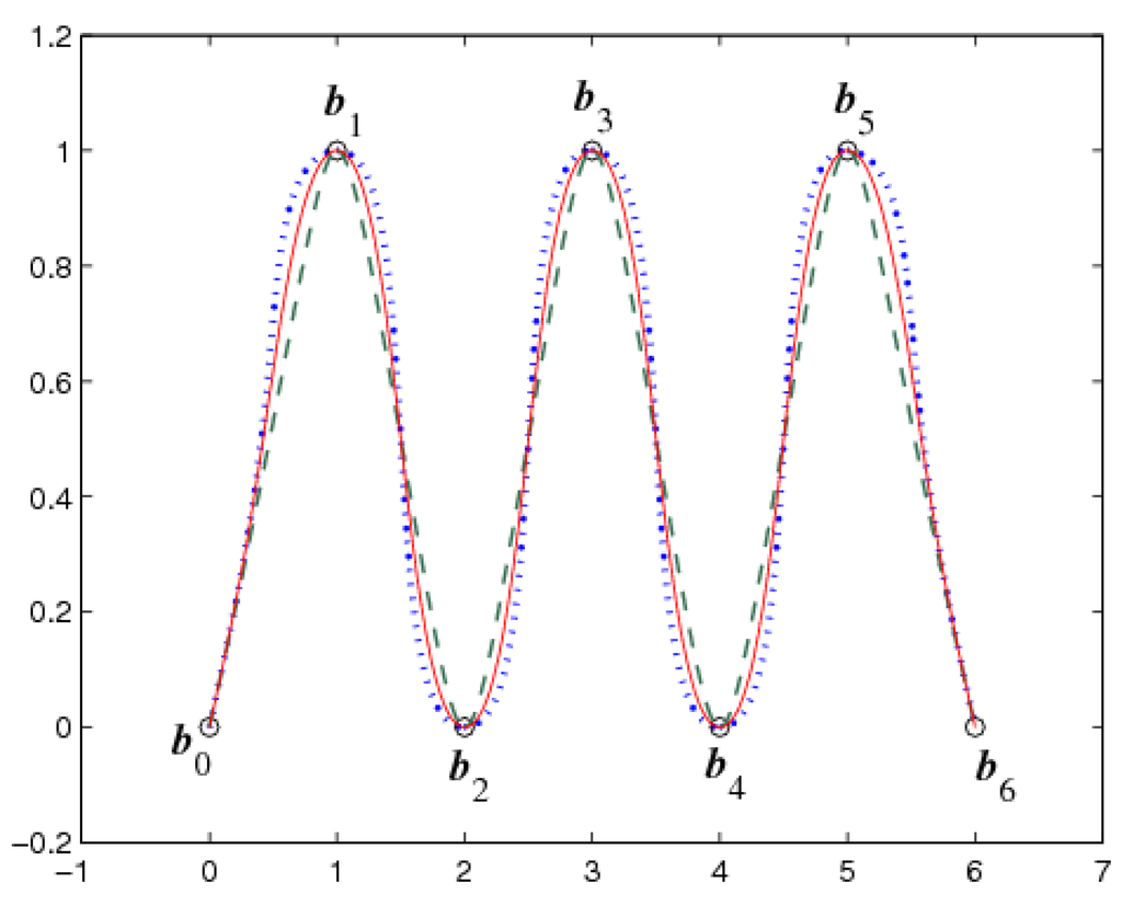
Consider the data points ${\mathit{b}}_0=(0,0)$, ${\mathit{b}}_1=(1,1)$, ${\mathit{b}}_2=(2,0)$, ${\mathit{b}}_3=(3,1)$, ${\mathit{b}}_4=(4,0)$, ${\mathit{b}}_5=(5,1)$, ${\mathit{b}}_6=(6,0)$, and two auxiliary points ${\mathit{b}}_{-1}=(-1,-1)$, ${\mathit{b}}_7=(7,-1)$. Open C² CTI-curves with different values of parameters α and β are shown in Figure 1, where the parameters are taken as $(\alpha ,\beta )=(-0.5,0.5)$ (marked with dotted lines), $(\alpha ,\beta )=(0,0)$ (marked with solid lines), and $(\alpha ,\beta )=(0.5,-0.5)$ (marked with dashed lines).

Figure 1. Open C² cubic trigonometric interpolation curves (CTI-curves) with different parameters.

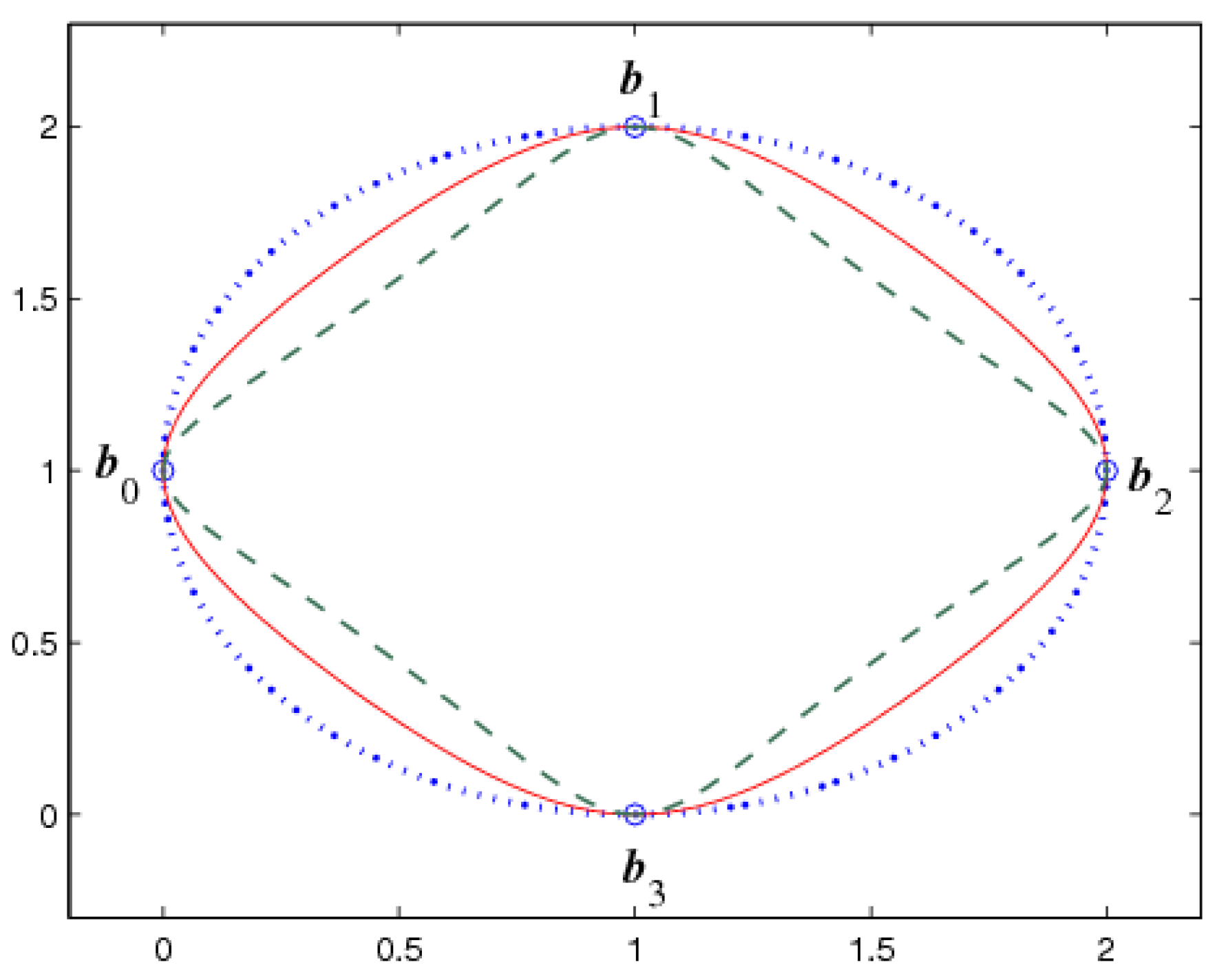
Example 2. 

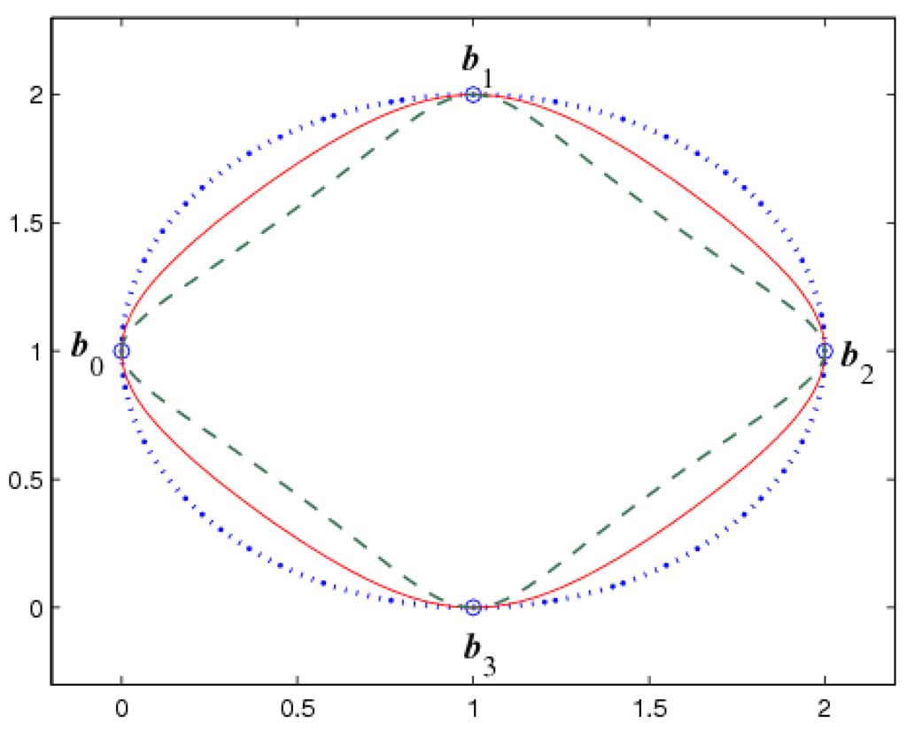
Consider the data points ${\mathit{b}}_0=(0,1)$, ${\mathit{b}}_1=(1,2)$, ${\mathit{b}}_2=(2,1)$, ${\mathit{b}}_3=(1,0)$, and three auxiliary points ${\mathit{b}}_{-1}=(1,0)$, ${\mathit{b}}_4=(0,1)$, ${\mathit{b}}_5=(1,2)$. Closed C² CTI-curves with different values of parameters α and β are shown in Figure 2, where the parameters are taken as $(\alpha ,\beta )=(-0.5,0.5)$ (marked with dotted lines), $(\alpha ,\beta )=(0,0)$ (marked with solid lines), and $(\alpha ,\beta )=(0.5,-0.5)$ (marked with dashed lines).

Figure 2. Closed C² CTI-curves with different parameters.

Remark 2. 

When using the traditional cubic spline to construct C² interpolation curves, the general way is to solve a linear equations system. However, due to the interpolation property and continuity of the CTI-curves, the interpolation curves can be generated naturally without solving an equations system. On the other hand, when the data points and auxiliary points are fixed, the traditional cubic interpolation curves are unique, while the CTI-curves can be adjusted by the parameters α and β.

Remark 3. 

Compared with some similar trigonometric interpolation curves (see in [13,14,15,16]), the CTI-curves presented in this paper have two outstanding characteristics,

(a)

Shapes of the CTI-curves can be adjusted by changing the parameters α and β even if data points and auxiliary points are kept unchanged.

(b)

The CTI-curves are not only C² but also have two degrees of freedom in the interpolation curves.

3.2. The Optimal Cti-Curves

The CTI-curves have two degrees of freedom. The shapes of the curves are determined by the parameters α and β when the data points and auxiliary points are fixed. Hence, bad interpolation curves would be generated if the parameters α and β are chosen improperly.

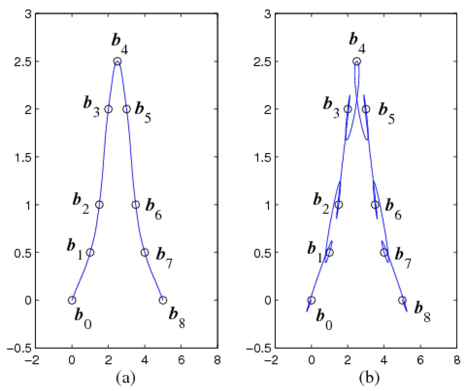
Example 3. 

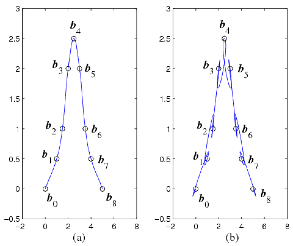
Consider the data points ${\mathit{b}}_0=(0,0)$, ${\mathit{b}}_1=(1,0.5)$, ${\mathit{b}}_2=(1.5,1)$, ${\mathit{b}}_3=(2,2)$, ${\mathit{b}}_4=(2.5,2.5)$, ${\mathit{b}}_5=(3,2)$, ${\mathit{b}}_6=(3.5,1)$, ${\mathit{b}}_7=(4,0.5)$, ${\mathit{b}}_8=(5,0)$, and two auxiliary points ${\mathit{b}}_{-1}=(-1,-0.5)$, ${\mathit{b}}_9=(6,-0.5)$. Figure 3 shows the CTI-curves with different values of parameters α and β for the same data points and auxiliary points, where the parameters are taken as (a): $(\alpha ,\beta )=(-0.1,0.2)$, (b): $(\alpha ,\beta )=(3.6,-2.8)$.

Figure 3. Effects of the parameters on CTI-curves. (a) $(\alpha ,\beta )=(-0.1,0.2)$ (b) $(\alpha ,\beta )=(3.6,-2.8)$ .

It is obvious that the interpolation curves in Figure 3a are more satisfactory than the interpolation curves in Figure 3b. Hence, how to determine proper parameters α and β of the CTI-curves is the key when constructing C² interpolation curves when the data points and auxiliary points are fixed. A method for determining the optimal parameters α and β of the CTI-curves is presented as follows.

When the CTI-curves are used to construct C² interpolation curves, the interpolation curves are usually required to be smooth. Generally, the smoothness of a curve can be measured by its energy. The lower the energy is, the smoother the curve. According to Reference [17], the energy value of a curve $\mathit{r}(t)$ $(a\le t\le b)$ can be approximately expressed as follows,

$$E_c={\displaystyle {\int }_a^b{\left({\mathit{r}}^{″}(t)\right)}^2}\mathrm{d}t$$

(7)

From Equation (7), for given data points ${\mathit{b}}_i$ $(i=0,1,\cdots ,n)$ and auxiliary points ${\mathit{b}}_{-1}$, ${\mathit{b}}_{n+1}$, the optimal parameters α and β of the CTI-curves ${\mathit{p}}_i(t)$ $(i=-1,0,1,\cdots ,n-2)$ can be determined by an energy optimization model expressed as follows,

$$\begin{array}{l}\begin{array}{cc}\min & E_c(\alpha ,\beta )={\displaystyle \sum _{i=-1}^{n-2}{\displaystyle {\int }_0^1{\left({\mathit{p}}_i^{″}(t)\right)}^2\mathrm{d}t}}\end{array}\\ \begin{array}{cc}\mathrm{s}.\text{t}.& \alpha ,\beta \in R\end{array}\end{array}$$

(8)

In order to obtain the minimum energy value, there must be

$$\{\begin{array}{l}\frac{\partial E_c}{\partial \alpha }=0\\ \frac{\partial E_c}{\partial \beta }=0\end{array}$$

(9)

Set

$$L_0(t)=\frac{1}{24}\left(-14+9S+24S^2-19S^3+14C^3\right),L_1(t)=\frac{1}{24}\left(2-9C-2S^3+7C^3\right),$$

$$L_2(t)=\frac{1}{24}\left(2-9S+7S^3-2C^3\right),L_3(t)=\frac{1}{24}\left(10+9C-24S^2+14S^3-19C^3\right),$$

$$M_0(t)=\frac{1}{24}\left(-2+3S-S^3+2C^3\right),M_1(t)=\frac{1}{24}\left(-10-3C+24S^2-14S^3+13C^3\right),$$

$$M_2(t)=\frac{1}{24}\left(14-3S-24S^2+13S^3-14C^3\right),M_3(t)=\frac{1}{24}\left(-2+3C+2S^3-C^3\right),$$

$$N_0(t)=\frac{1}{24}\left(6-9S+3S^3-6C^3\right),N_1(t)=\frac{1}{24}\left(6+9C-6S^3+9C^3\right),$$

$$N_2(t)=\frac{1}{24}\left(6+9S+9S^3-6C^3\right),N_3(t)=\frac{1}{24}\left(6-9C-6S^3+3C^3\right),$$

where $S:=\sin \frac{\pi t}{2}$, $C:=\cos \frac{\pi t}{2}$, $0\le t\le 1$. Then, Equation (2) can be rewritten as follows,

$${\mathit{p}}_i(t)={\mathit{G}}_i(t)\alpha +{\mathit{H}}_i(t)\beta +{\mathit{I}}_i(t)$$

(10)

where

$${\mathit{G}}_i(t)=L_0(t){\mathit{b}}_i+L_1(t){\mathit{b}}_{i+1}+L_2(t){\mathit{b}}_{i+2}+L_3(t){\mathit{b}}_{i+3},$$

$${\mathit{H}}_i(t)=M_0(t){\mathit{b}}_i+M_1(t){\mathit{b}}_{i+1}+M_2(t){\mathit{b}}_{i+2}+M_3(t){\mathit{b}}_{i+3},$$

$${\mathit{I}}_i(t)=N_0(t){\mathit{b}}_i+N_2(t){\mathit{b}}_{i+1}+N_3(t){\mathit{b}}_{i+2}+N_4(t){\mathit{b}}_{i+3}.$$

From Equation (10), Equation (7) can be expressed as follows,

$$E_c=C_1{\alpha }^2+C_2{\beta }^2+2C_3\alpha \beta +2C_4\alpha +2C_5\beta +C_6$$

(11)

where

$${\mathit{C}}_1={\displaystyle \sum _{i=0}^{n-3}{\displaystyle {\int }_0^1{\left({\mathit{G}}_i^{″}(t)\right)}^2}}\mathrm{d}t,C_2={\displaystyle \sum _{i=0}^{n-3}{\displaystyle {\int }_0^1{\left({\mathit{H}}_i^{″}(t)\right)}^2}}\mathrm{d}t,C_3={\displaystyle \sum _{i=0}^{n-3}{\displaystyle {\int }_0^1\left({\mathit{G}}_i^{″}(t)\cdot {\mathit{H}}_i^{″}(t)\right)}}\mathrm{d}t,$$

$$C_4={\displaystyle \sum _{i=0}^{n-3}{\displaystyle {\int }_0^1\left({\mathit{G}}_i^{″}(t)\cdot {\mathit{I}}_i^{″}(t)\right)}}\mathrm{d}t,C_5={\displaystyle \sum _{i=0}^{n-3}{\displaystyle {\int }_0^1\left({\mathit{H}}_i^{″}(t)\cdot {\mathit{I}}_i^{″}(t)\right)}}\mathrm{d}t,C_6={\displaystyle \sum _{i=0}^{n-3}{\displaystyle {\int }_0^1{\left({\mathit{I}}_i^{″}(t)\right)}^2}}\mathrm{d}t.$$

By Equation (11), Equation (9) can be rewritten as follows,

$$\{\begin{array}{l}{C}_1\alpha +C_3\beta +C_4=0\\ C_3\alpha +C_2\beta +C_5=0\end{array}$$

(12)

When $C_1{C}_2-C_3^2\ne 0$, from Equation (12), then

$$\{\begin{array}{l}\alpha =\frac{C_3{C}_5-C_2{C}_4}{C_1{C}_2-C_3^2}\\ \beta =\frac{C_3{C}_4-C_1{C}_5}{C_1{C}_2-C_3^2}\end{array}$$

(13)

Remark 4. 

If $C_1{C}_2-C_3^2=0$, there would be no unique solution to Equation (13). At this point, the two auxiliary points could be adjusted properly in order to ensure that $C_1{C}_2-C_3^2\ne 0$ holds.

After the optimal parameters $\alpha =\tilde{\alpha }$ and $\beta =\tilde{\beta }$ are determined by Equation (13), the optimal C² CTI-curves ${\tilde{\mathit{p}}}_i(t)$ $(i=-1,0,1,\cdots ,n-2)$ interpolating all the given data points ${\mathit{b}}_i$ $(i=0,1,\cdots ,n)$ can be obtained.

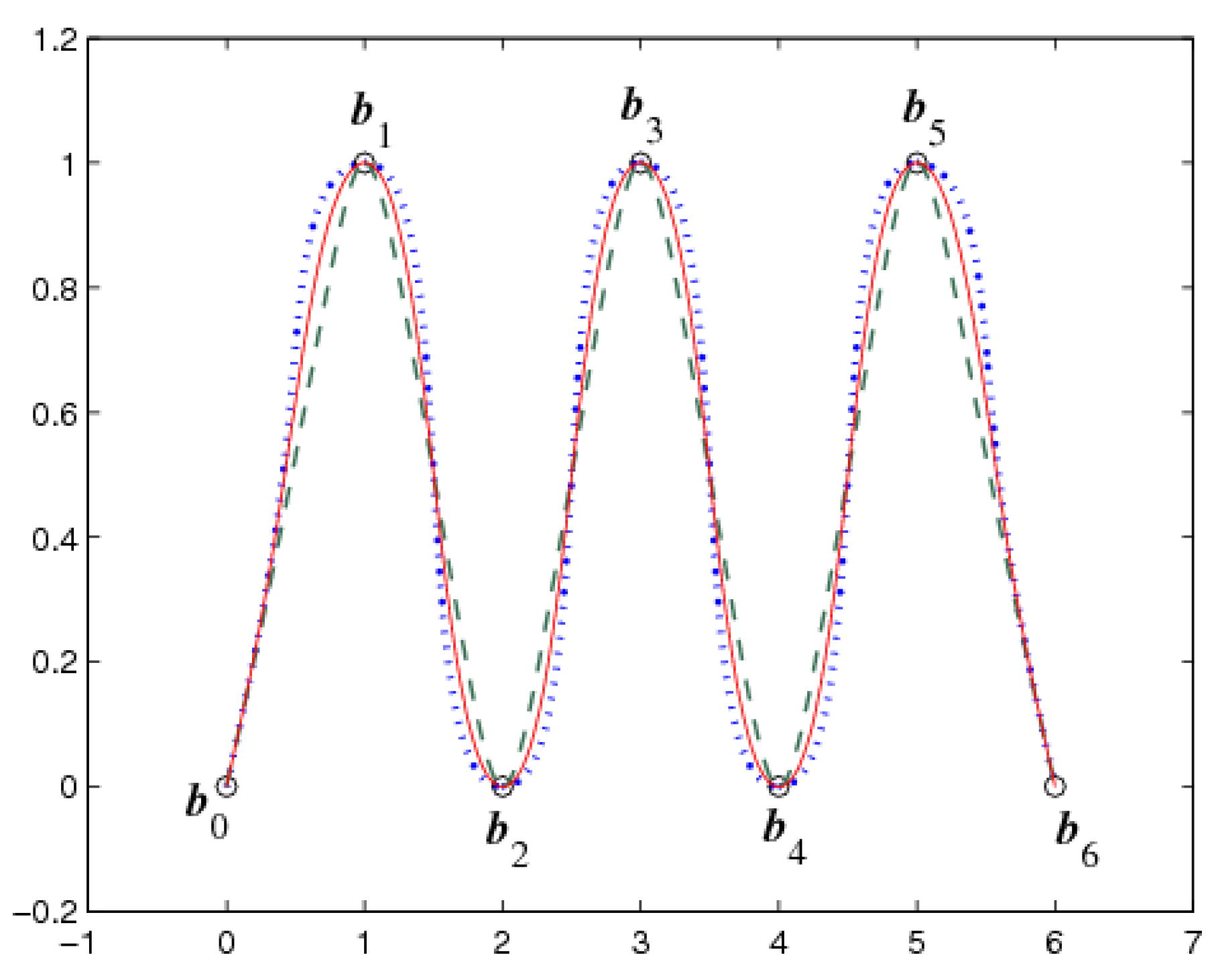
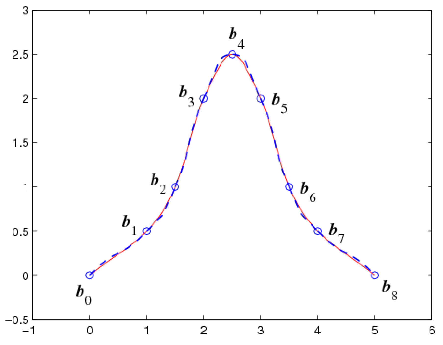
Example 4. 

For the same data points and auxiliary points in Example 3, the optimal parameters of the CTI-curves, determined by Equation (13), are $\tilde{\alpha }=-0.0443$ and $\tilde{\beta }=0.4836$. The optimal C² CTI-curves (solid lines) and the interpolation curves constructed by the classical cubic B-spline curves (dashed lines) are shown in Figure 4, where the tangent vectors at the endpoints of the classical cubic B-spline curves are taken as $3({\mathit{b}}_0-{\mathit{b}}_{-1})$ and $3({\mathit{b}}_9-{\mathit{b}}_8)$.

Figure 4. The optimal C² CTI-curves.

For comparing the CTI-curves with the classical cubic B-spline curves to construct interpolation curves, the energy values and time-consuming of the two methods are shown in Table 1.

Table 1. The energy values and time-consuming of the two methods.

Method	Energy Value	Time-Consuming (s)
CTI-curves	4.8584	9.6
Classical cubic B-spline curves	17.6137	16.3

Table 1 shows that the interpolation curves constructed by the CTI-curves are smoother and faster to compute than the classical cubic B-spline curves.

4. The CTI-Surfaces

Using tensor products, the corresponding CTI-surfaces can be defined as follows.

Definition 3. 

Given data points ${\mathit{b}}_{k,l}$ $(k=0,1,\cdots ,m;l=0,1,\cdots ,n)$ in ${\mathbf{R}}^3$, the piecewise surfaces

$${\mathit{p}}_{i,j}(u,v)={\displaystyle \sum _{k=0}^3{\displaystyle \sum _{l=0}^3{f}_k(u)}{f}_l(v)}{\mathit{b}}_{i+k,j+l}$$

(14)

are called cubic trigonometric interpolation surfaces with parameters ${\alpha }_1$, ${\beta }_1$, ${\alpha }_2$ and ${\beta }_2$ (CTI-surfaces for short), where $i=0,1,\cdots ,m-3$, $j=0,1,\cdots ,n-3$, $f_k(u):=f_k(u;{\alpha }_1,{\beta }_1)$ and $f_l(v):=f_l(v;{\alpha }_2,{\beta }_2)$ $(i=0,1,2,3)$ are the CTI-basis functions defined according to Equation (1).

It is not difficult to show that the CTI-surfaces have properties similar to the CTI-curves, which include the following important property.

Theorem 2. 

Given data points ${\mathit{b}}_{k,l}$ $(k=0,1,\cdots ,m;l=0,1,\cdots ,n)$, the CTI-surfaces ${\mathit{p}}_{i,j}(u,v)$ ($i=0,1,\cdots ,m-3$; $j=0,1,\cdots ,n-3$) automatically interpolate all the given data points except ${\mathit{b}}_{0,l}$, ${\mathit{b}}_{m,l}$ $(l=0,1,\cdots ,n)$ and $b_{k,0}$, $b_{k,n}$ $(k=0,1,\cdots ,m)$ and are C².

Proof. 

From the properties at the endpoints of the CTI-basis functions and Equation (14),

$$\{\begin{array}{l}{\mathit{p}}_{i,j}(0,0)={\mathit{b}}_{i+1,j+1}\\ {\mathit{p}}_{i,j}(0,1)={\mathit{b}}_{i+1,j+2}\\ {\mathit{p}}_{i,j}(1,0)={\mathit{b}}_{i+2,j+1}\\ {\mathit{p}}_{i,j}(1,1)={\mathit{b}}_{i+2,j+2}\end{array}$$

(15)

$$\{\begin{array}{l}{\partial }_u{\mathit{p}}_{i,j}(0,v)=\frac{\pi }{16}{\displaystyle \sum _{l=0}^3{f}_l(v)(}{\mathit{b}}_{i+2,j+l}-{\mathit{b}}_{i,j+l})\\ {\partial }_u{\mathit{p}}_{i,j}(1,v)=\frac{\pi }{16}{\displaystyle \sum _{l=0}^3{f}_l(v)(}{\mathit{b}}_{i+3,j+l}-{\mathit{b}}_{i+1,j+l})\\ {\partial }_u{\mathit{p}}_{i,j}(u,0)={\displaystyle \sum _{k=0}^3{f}_k^{\prime }(u)}{\mathit{b}}_{i+k,j+1}\\ {\partial }_u{\mathit{p}}_{i,j}(u,1)={\displaystyle \sum _{k=0}^3{f}_k^{\prime }(u)}{\mathit{b}}_{i+k,j+2}\end{array}$$

(16)

$$\{\begin{array}{l}{\partial }_v{\mathit{p}}_{i,j}(0,v)={\displaystyle \sum _{l=0}^3{f}_l^{\prime }(v)}{\mathit{b}}_{i+1,j+l}\\ {\partial }_v{\mathit{p}}_{i,j}(1,v)={\displaystyle \sum _{l=0}^3{f}_l^{\prime }(v)}{\mathit{b}}_{i+2,j+l}\\ {\partial }_v{\mathit{p}}_{i,j}(u,0)=\frac{\pi }{16}{\displaystyle \sum _{k=0}^3{f}_k(u)(}{\mathit{b}}_{i+k,j+2}-{\mathit{b}}_{i+k,j})\\ {\partial }_v{\mathit{p}}_{i,j}(u,1)=\frac{\pi }{16}{\displaystyle \sum _{k=0}^3{f}_k(u)(}{\mathit{b}}_{i+k,j+3}-{\mathit{b}}_{i+k,j+1})\end{array}$$

(17)

$$\{\begin{array}{l}{\partial }_{uv}{\mathit{p}}_{i,j}(0,v)=\frac{\pi }{16}{\displaystyle \sum _{l=0}^3{f}_l^{\prime }(v)(}{\mathit{b}}_{i+2,j+l}-{\mathit{b}}_{i,j+l})\\ {\partial }_{uv}{\mathit{p}}_{i,j}(1,v)=\frac{\pi }{16}{\displaystyle \sum _{l=0}^3{f}_l^{\prime }(v)(}{\mathit{b}}_{i+3,j+l}-{\mathit{b}}_{i+1,j+l})\\ {\partial }_{uv}{\mathit{p}}_{i,j}(u,0)=\frac{\pi }{16}{\displaystyle \sum _{k=0}^3{f}_k^{\prime }(u)(}{\mathit{b}}_{i+k,j+2}-{\mathit{b}}_{i+k,j})\\ {\partial }_{uv}{\mathit{p}}_{i,j}(u,1)=\frac{\pi }{16}{\displaystyle \sum _{k=0}^3{f}_k^{\prime }(u)(}{\mathit{b}}_{i+k,j+3}-{\mathit{b}}_{i+k,j+1})\end{array}$$

(18)

$$\{\begin{array}{l}{\partial }_{uu}{\mathit{p}}_{i,j}(0,v)=\frac{{\pi }^2}{16}{\displaystyle \sum _{l=0}^3{f}_l(v)(}{\mathit{b}}_{i,j+l}-2{\mathit{b}}_{i+1,j+l}+{\mathit{b}}_{i+2,j+l})\\ {\partial }_{uu}{\mathit{p}}_{i,j}(1,v)=\frac{{\pi }^2}{16}{\displaystyle \sum _{l=0}^3{f}_l(v)(}{\mathit{b}}_{i+1,j+l}-2{\mathit{b}}_{i+2,j+l}+{\mathit{b}}_{i+3,j+l})\\ {\partial }_{uu}{\mathit{p}}_{i,j}(u,0)={\displaystyle \sum _{k=0}^3{f}_k^{″}(u)}{\mathit{b}}_{i+k,j+1}\\ {\partial }_{uu}{\mathit{p}}_{i,j}(u,1)={\displaystyle \sum _{k=0}^3{f}_k^{″}(u)}{\mathit{b}}_{i+k,j+2}\end{array}$$

(19)

$$\{\begin{array}{l}{\partial }_{vv}{\mathit{p}}_{i,j}(0,v)={\displaystyle \sum _{l=0}^3{f}_l^{″}(v)}{\mathit{b}}_{i+1,j+l}\\ {\partial }_{vv}{\mathit{p}}_{i,j}(1,v)={\displaystyle \sum _{l=0}^3{f}_l^{″}(v)}{\mathit{b}}_{i+2,j+l}\\ {\partial }_{vv}{\mathit{p}}_{i,j}(u,0)=\frac{{\pi }^2}{16}{\displaystyle \sum _{k=0}^3{f}_k(u)(}{\mathit{b}}_{i+k,j}-2{\mathit{b}}_{i+k,j+1}+{\mathit{b}}_{i+k,j+2})\\ {\partial }_{vv}{\mathit{p}}_{i,j}(u,1)=\frac{{\pi }^2}{16}{\displaystyle \sum _{k=0}^3{f}_k(u)(}{\mathit{b}}_{i+k,j+1}-2{\mathit{b}}_{i+k,j+2}+{\mathit{b}}_{i+k,j+3})\end{array}$$

(20)

Equation (15) shows that the CTI-surfaces ${\mathit{p}}_{i,j}(u,v)$ ($i=0,1,\cdots ,m-3$; $j=0,1,\cdots ,n-3$) automatically interpolate all the given data points except ${\mathit{b}}_{0,l}$, ${\mathit{b}}_{m,l}$ $(l=0,1,\cdots ,n)$ and ${\mathit{b}}_{k,0}$, ${\mathit{b}}_{k,n}$ $(k=0,1,\cdots ,m)$. In addition, the following results can also be obtained from Equation (15),

$$\{\begin{array}{l}{\mathit{p}}_{i,j}(1,0)={\mathit{p}}_{i+1,j}(0,0)\\ {\mathit{p}}_{i,j}(1,1)={\mathit{p}}_{i+1,j}(0,1)\\ {\mathit{p}}_{i,j}(0,1)={\mathit{p}}_{i,j+1}(0,0)\\ {\mathit{p}}_{i,j}(1,1)={\mathit{p}}_{i,j+1}(1,0)\end{array}$$

(21)

From Equations (16) and (17),

$$\{\begin{array}{l}{\partial }_u{\mathit{p}}_{i,j}(1,v)={\partial }_u{\mathit{p}}_{i+1,j}(0,v)\\ {\partial }_u{\mathit{p}}_{i,j}(u,1)={\partial }_u{\mathit{p}}_{i,j+1}(u,0)\\ {\partial }_v{\mathit{p}}_{i,j}(1,v)={\partial }_v{\mathit{p}}_{i+1,j}(0,v)\\ {\partial }_v{\mathit{p}}_{i,j}(u,1)={\partial }_v{\mathit{p}}_{i,j+1}(u,0)\end{array}$$

(22)

From Equations (18)–(20),

$$\{\begin{array}{l}{\partial }_{uv}{\mathit{p}}_{i,j}(1,v)={\partial }_{uv}{\mathit{p}}_{i+1,j}(0,v)\\ {\partial }_{uv}{\mathit{p}}_{i,j}(u,1)={\partial }_{uv}{\mathit{p}}_{i,j+1}(u,0)\\ {\partial }_{uu}{\mathit{p}}_{i,j}(1,v)={\partial }_{uu}{\mathit{p}}_{i+1,j}(0,v)\\ {\partial }_{uu}{\mathit{p}}_{i,j}(u,1)={\partial }_{uu}{\mathit{p}}_{i,j+1}(u,0)\\ {\partial }_{vv}{\mathit{p}}_{i,j}(1,v)={\partial }_{vv}{\mathit{p}}_{i+1,j}(0,v)\\ {\partial }_{vv}{\mathit{p}}_{i,j}(u,1)={\partial }_{vv}{\mathit{p}}_{i,j+1}(u,0)\end{array}$$

(23)

Equations (21)–(23) show that the CTI-surfaces ${\mathit{p}}_{i,j}(u,v)$ ($i=0,1,\cdots ,m-3$; $j=0,1,\cdots ,n-3$) are C².

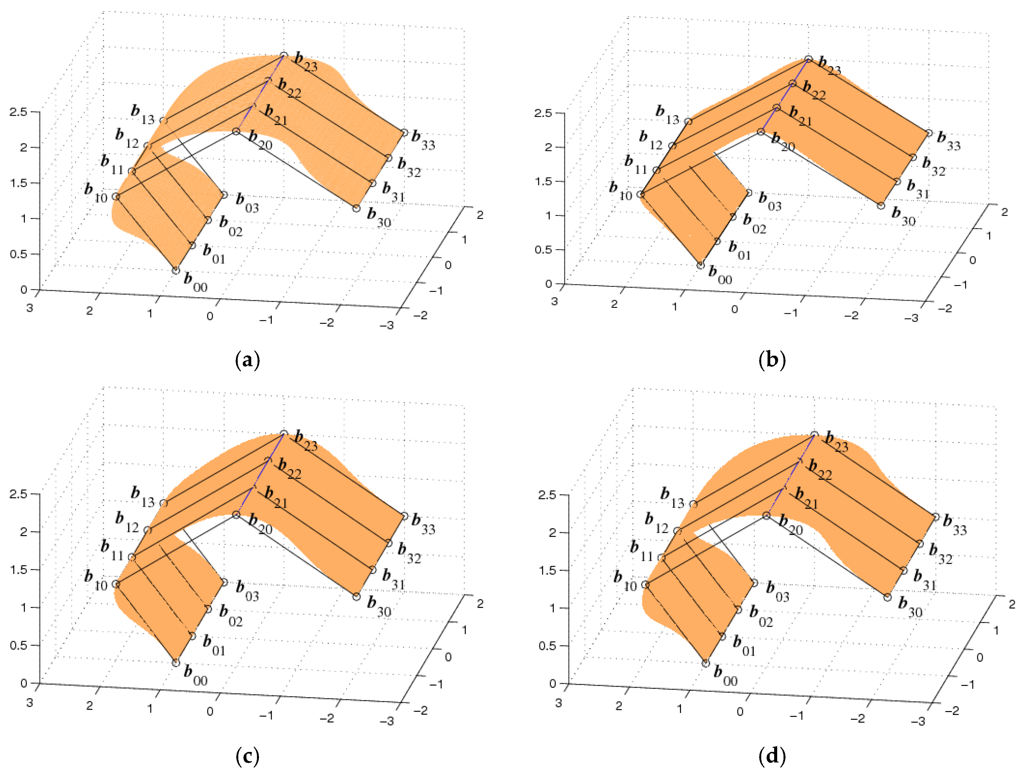
According to Theorem 2, for given data points ${\mathit{b}}_{k,l}$ $(k=0,1,\cdots ,m;l=0,1,\cdots ,n)$, the CTI-surfaces automatically interpolate all the given data points except ${\mathit{b}}_{0,l}$, ${\mathit{b}}_{m,l}$ $(l=0,1,\cdots ,n)$ and ${\mathit{b}}_{k,0}$, ${\mathit{b}}_{k,n}$ $(k=0,1,\cdots ,m)$. If auxiliary points ${\mathit{b}}_{-1,j}$, ${\mathit{b}}_{m+1,j}$ $(j=0,1,\cdots ,n)$ and ${\mathit{b}}_{i,-1}$, ${\mathit{b}}_{i,n+1}$ $(i=0,1,\cdots ,m)$ are added to the given data points, the C² CTI-surfaces interpolating all the data points ${\mathit{b}}_{k,l}$ $(k=0,1,\cdots ,m;l=0,1,\cdots ,n)$ would be generated naturally. Generally, the auxiliary points can be taken as follows,

$$\{\begin{array}{l}\begin{array}{cc}{\mathit{b}}_{-1,-1}=2{\mathit{b}}_{0,0}-{\mathit{b}}_{1,1},& {\mathit{b}}_{-1,n+1}=2{\mathit{b}}_{0,n}-{\mathit{b}}_{1,n-1}\end{array}\\ {\mathit{b}}_{m+1,-1}=2{\mathit{b}}_{m,0}-{\mathit{b}}_{m-1,1},\hspace{1em}{\mathit{b}}_{m+1,n+1}=2{\mathit{b}}_{m,n}-{\mathit{b}}_{m-1,n-1}\\ \begin{array}{ccc}{\mathit{b}}_{-1,j}=2{\mathit{b}}_{0,j}-{\mathit{b}}_{1,j},& {\mathit{b}}_{m+1,j}=2{\mathit{b}}_{m,j}-{\mathit{b}}_{m-1,j},& j=0,1,\cdots ,n\end{array}\\ \begin{array}{ccc}{\mathit{b}}_{i,-1}=2{\mathit{b}}_{i,0}-{\mathit{b}}_{i,1},& {\mathit{b}}_{i,n+1}=2{\mathit{b}}_{i,n}-{\mathit{b}}_{i,n-1},& i=0,1,\cdots ,m\end{array}\end{array}$$

(24)

It is clear that there exist four degrees of freedom in the C² CTI-surfaces, even if the data points and auxiliary points are fixed. Different interpolation results can be obtained by altering the parameters ${\alpha }_i$ and ${\beta }_i$ $(i=1,2)$ of the CTI-surfaces. Figure 5 shows the C² CTI-surfaces with different values of parameters ${\alpha }_i$ and ${\beta }_i$ $(i=1,2)$, where the data points ${\mathit{b}}_{k,l}$ $(k=0,1,2,3;l=0,1,2,3)$ are fixed and the auxiliary points are added according to Equation (24).

Figure 5. C² CTI-surfaces with different parameters. (a) $({\alpha }_1,{\beta }_1,{\alpha }_2,{\beta }_2)=(-0.5,0.5,0.5,-0.5)$ ; (b) $({\alpha }_1,{\beta }_1,{\alpha }_2,{\beta }_2)=(0.5,-0.5,-0.5,0.5)$ ; (c) $({\alpha }_1,{\beta }_1,{\alpha }_2,{\beta }_2)=(0.1,-0.5,0.4,-0.3)$ ; (d) $({\alpha }_1,{\beta }_1,{\alpha }_2,{\beta }_2)=(-0.3,0,0,0.4)$ .

Similar to the optimal CTI-curves, the optimal CTI-surfaces can also be determined by an energy optimization model. According to Ref. [17], the energy value of a surface $\mathit{r}(u,v)$ $(a\le u\le b,c\le v\le d)$ can be approximately expressed as follows,

$$E_s={\displaystyle {\int }_a^b{\displaystyle {\int }_c^d\left({\left({\mathit{r}}_{uu}(u,v)\right)}^2+2{\left({\mathit{r}}_{uv}(u,v)\right)}^2+{\left({\mathit{r}}_{vv}(u,v)\right)}^2\right)}}\mathrm{d}u\mathrm{d}v$$

(25)

From Equation (25), for given data points ${\mathit{b}}_{k,l}$ $(k=0,1,\cdots ,m;l=0,1,\cdots ,n)$ and auxiliary points ${\mathit{b}}_{-1,j}$, ${\mathit{b}}_{m+1,j}$ $(j=0,1,\cdots ,n)$, ${\mathit{b}}_{i,-1}$, ${\mathit{b}}_{i,n+1}$ $(i=0,1,\cdots ,m)$, the optimal parameters ${\alpha }_i$ and ${\beta }_i$ $(i=1,2)$ of the CTI-surfaces ${\mathit{p}}_{i,j}(u,v)$ $(i=-1,0,1,\cdots ,m-2;j=-1,0,1,\cdots ,n-2)$ can be determined by an energy optimization model expressed as follows,

$$\begin{array}{l}\begin{array}{cc}\min & E_s({\alpha }_1,{\beta }_1,{\alpha }_2,{\beta }_2)={\displaystyle \sum _{i=-1}^{m-2}{\displaystyle \sum _{j=-1}^{n-2}{\displaystyle {\int }_0^1{\displaystyle {\int }_0^1\left({\left(\frac{{\partial }^2{\mathit{p}}_{i,j}(u,v)}{\partial u^2}\right)}^2+2{\left(\frac{{\partial }^2{\mathit{p}}_{i,j}(u,v)}{\partial u\partial v}\right)}^2+{\left(\frac{{\partial }^2{\mathit{p}}_{i,j}(u,v)}{\partial v^2}\right)}^2\right)}\mathrm{d}u\mathrm{d}v}}}\end{array}\\ \begin{array}{cc}\mathrm{s}.\text{t}.& {\alpha }_1,{\beta }_1,{\alpha }_2,{\beta }_2\in R\end{array}\end{array}$$

(26)

The particle swarm optimization (PSO) algorithm [18] can be used to solve Equation (26). After the optimal parameters ${\alpha }_i={\tilde{\alpha }}_i$ and ${\beta }_i={\tilde{\beta }}_i$ $(i=1,2)$ are determined, the optimal C² CTI-surfaces ${\tilde{\mathit{p}}}_{i,j}(u,v)$ $(i=-1,0,1,\cdots ,m-2;j=-1,0,1,\cdots ,n-2)$ interpolating all the given data points ${\mathit{b}}_{k,l}$ $(k=0,1,\cdots ,m;l=0,1,\cdots ,n)$ can be obtained.

5. Conclusions

The CTI-curves presented in this paper can not only automatically interpolate the given data points without solving equation systems, but are also C² and have two degrees of freedom. The CTI-surfaces also have characteristics similar to the CTI-curves. Therefore, the CTI-curves/surfaces presented in this paper provide a simple and efficient way for constructing interpolation curves and surfaces.

For practical applications of the proposed interpolation curves and surfaces in geometric modeling, it is clear that some special algorithms need to be established. Furthermore, the proposed interpolation curves and surfaces allow only global adjustment. Hence, local adjustment of the proposed interpolation curves and surfaces also need to be investigated. Some interesting results in this area will be presented in a follow-up study.

References

- Hoschek, J.; Lasser, D. Fundamentals of Computer Aided Geometric Design; Schumaker, L.L., Translator; A.K. Peters, Ltd.: Natick, MA, USA, 1993. [Google Scholar]
- Han, X.L. Cubic trigonometric polynomial curves with a shape parameter. Comput. Aided Geom. Des. 2004, 21, 535–548. [Google Scholar] [CrossRef]
- Zhang, J.W.; Krause, F.L. Extending cubic uniform B-splines by unified trigonometric and hyperbolic basis. Gr. Model. 2005, 67, 100–119. [Google Scholar] [CrossRef]
- Mainar, E. A general class of Bernstein-like bases. Comput. Math. Appl. 2007, 53, 1686–1703. [Google Scholar] [CrossRef]
- Wang, G.Z.; Fang, M.E. Unified and extended form of three types of splines. J. Comput. Appl. Math. 2008, 216, 498–508. [Google Scholar] [CrossRef]
- Han, X.A.; Ma, Y.C.; Huang, X.L. The cubic trigonometric Bézier curve with two shape parameters. Appl. Math. Lett. 2009, 22, 226–231. [Google Scholar] [CrossRef]
- Han, X.L.; Zhu, Y.P. Curve construction based on five trigonometric blending functions. BIT Numer. Math. 2012, 52, 953–979. [Google Scholar] [CrossRef]
- Bashir, U.; Abbsa, M.; Ali, J.M. The G2 and C2 rational quadratic trigonometric Bézier curve with two shape parameters with applications. Appl. Math. Comput. 2013, 219, 10183–10197. [Google Scholar] [CrossRef]
- Bashir, U.; Ali, J.M. Rational cubic trigonometrc Bézier curve with two shape parameters. Comput. Appl. Math. 2016, 35, 285–300. [Google Scholar] [CrossRef]
- Han, X.L. Normalized B-basis of the space of trigonometric polynomials and curve design. Appl. Math. Comput. 2015, 251, 336–348. [Google Scholar] [CrossRef]
- Yan, L.L. An algebraic-trigonometric blended piecewise curve. J. Infor. Comput. Sci. 2015, 12, 6491–6501. [Google Scholar] [CrossRef]
- Yan, L.L. Cubic trigonometric nonuniform spline curves and surfaces. Math. Probl. Eng. 2016, 2016, 1–9. [Google Scholar] [CrossRef]
- Su, B.Y.; Tan, J.Q. A family of quasi-cubic blended splines and applications. J. Zhejiang Univ. Sci. A 2006, 7, 1550–1560. [Google Scholar] [CrossRef]
- Yan, L.L.; Liang, J.F. A class of algebraic-trigonometric blended splines. J. Comput. Appl. Math. 2011, 235, 1713–1729. [Google Scholar] [CrossRef]
- Li, J.C.; Zhao, D.B.; Yang, L. Quasi-cubic trigonometric spline interpolation curves and surfaces. J. Chin. Comput. Syst. 2013, 34, 680–684. (In Chinese) [Google Scholar]
- Yang, L.; Li, J.C.; Kuang, X.L. A family of local adjustable cubic algebraic-trigonometric interpolation spline. Comput. Eng. Sci. 2013, 35, 130–135. (In Chinese) [Google Scholar]
- Poliakoff, J.F. An improved algorithm for automatic fairing of non-uniform parametric cubic splines. Comput. Aided Des. 1996, 28, 59–66. [Google Scholar] [CrossRef]
- Eberhart, R.C.; Kennedy, J. A new optimizer using particle swarm theory. In Proceedings of the Sixth International Symposium on Micro Machine and Human Science, Nagoya, Japan, 4–6 October 1995; pp. 39–43.
© 2016 by the author; licensee MDPI, Basel, Switzerland. This article is an open access article distributed under the terms and conditions of the Creative Commons Attribution (CC-BY) license (http://creativecommons.org/licenses/by/4.0/).