Abstract
Grid turbulence is considered to be a canonical case of turbulent flow. In the presented paper, the flow structure is analyzed from the point of view of mixing properties, where vortical structures and their properties play a significant role. That is why the effect of various length-scales in turbulence is studied separately. The experimental study uses the Particle Image Velocimetry (PIV) method. The original method for spatial spectrum evaluation is applied. Results on vortex spatial spectrum and isotropy are presented. The scaling of turbulent kinetic energy (TKE) is measured; furthermore, the TKE is decomposed according to the length-scales of the fluctuations. By this method, we found that the decay of TKE associated with the smallest length-scales is more sensitive to the Reynolds number than that at larger length-scales. The TKE at the largest investigated length-scales decays more slowly. The turbulence decay-law is studied for various Reynolds numbers. The second and fourth statistical moments of vorticity are evaluated at various Reynolds numbers and distances from the grid. The isotropy is investigated in the sense of ratio of fluctuations in stream-wise to span-wise directions as the used data are captured using the planar PIV method. The full 3D fluctuation invariants were investigated in a representative position by means of the Stereo-PIV method.
1. Introduction
Turbulence is the most common form of moving fluid behavior in nature and technology. This complex phenomenon could be characterized by number of attributes, among them randomness and multi-scale structure. The turbulent flow consists of a complex system of vortices with small random eddies being embedded in larger ones. One of the most important turbulence properties used in technological applications is its ability to substantially enhance mixing process. However, the turbulence mixing efficiency depends strongly on its structure, namely on vortices sizes and other parameters [].
Grid turbulence is a widely studied prototype of almost ideal Kolmogorov-style homogeneous and isotropic turbulence. In reality, grid turbulence provides only a rough approximation to homogenous isotropic turbulence. While the small scales satisfy isotropy to a close approximation, larger scales exhibit a non-negligible departure from isotropy, []. The statistical characterization of the passive scalar field in turbulent conditions also reveals a strong small scale intermittency, with important and uneven fluctuations of the scalar dissipation []. The origins of this intermittency and its connection to the intermittency of the carrier flow remain open questions.
In spite of long-time systematical research performed experimentally of this type of flow, there are still attempts to clarify the details of turbulence behavior. For example, there is a recent unique study on this subject using large scale experiment, see [].
A closer look shows the system of wakes and jets in the near-grid region; wakes form past the grid rods, while jets for past the grid holes. When the growing wakes meet (or the narrowing jet cores disappear), the turbulence start to homogenize forming vortices even larger than the mesh size (e.g., distance of the neighboring rods; here denoted M) via the inverse cascade. In the developed region, the homogenization is completed, while the isotropy condition seems not to be fulfilled. The Richardson cascade transfers energy mainly from large scales to smaller scales, where it converges into heat via molecular viscosity. A consequence is that the turbulence decays from the bottom, meaning that the small vortices disappear first, leaving the larger vortices there. In other words, the Kolmogorov dissipative scale grows in time, or in space in the case of continuous flow through a channel.
From the mixing point of view, the grid turbulence offers a relatively low-pressure-loss possibility of intensifying mixing inside a channel (or pipe). On the other hand, the mixing scales are not ideally distributed. —First, in the near region of distinguished wakes and jets, there is intense mixing over small scales inside the wakes but the large-scale volumes stay separated; later, there are vortices larger than the mesh parameter M, which mix the distant volumes well, but the growing Kolmogorov scale leaves a gap between the smallest turbulent scale and the scale of molecular diffusivity.
The presented study is a contribution to clarify the behavior of various scales, i.e., vortices with various sizes, in turbulence. This aspect is essential for effectivity of mixing.
In the Section 2 the used materials and methods are addressed. There is description of employed experimental facility and methods. Special attention is devoted to the grid geometry, as this forms an important part of boundary conditions for the flow. The Section 3 is about results. The Turbulent kinetic energy and its decay is addressed with special attention to theirs scales. Then vorticity development is studied and isotropy of the turbulence as the last analysis. In the Appendix A, the method of turbulent kinetic energy from 2 velocity components is discussed. The conclusions sum-up the results.
2. Materials and Methods
2.1. The Grid
The grid used for generating turbulence has a square symmetry of square holes divided by rods of square cross-section, see Figure 1, with a cylinder fitted into this corner and with a radius of , (although a sharp corner was intended here), in part (b). The distance of the rods is the mesh parameter , which is a base length unit used in grid-turbulence studies. The side of the rods is denoted . The porosity defined as the ratio of free area to the total area is
Figure 1.
(a) Scan of the entire grid produced by using a 3D printer. (b) Zoomed-in image of one of the corners. Blue arrow shows the stream-wise direction.
The grid is placed in the inlet of the wind tunnel test-section. The geometry has been prepared within the language OpenSCAD, whose applicability for scientific modeling has been explored in more detail, e.g., in []. The grid was manufactured by using 3D printer Prusa Mk2.5 and it was made from polymerized lactic acid (PLA) [].
The majority of studies just state the planed geometry, but, in reality, the actual shape differs from the projected one due to the finite precision of manufacturing processes. In this study we measure the actual geometry.
2.2. Optical Scanning
The method of 3D optical scanning is based on stereo capture of multiple photos of a given object, which has to be scanned. We use a commercially available 3D optical scanner Gom Atos Core, which allows us to scan volumes up to with micrometer resolution. It projects a blue-light pattern to the measured surface, the deformation of a such pattern is measured by using a pair of high-resolution cameras reconstructing the 3D shape of the object. As the entire shape cannot be covered, multiple scans from different directions are applied. In order to match these scans well, small printed points are used and identified uniquely by comparing triangles made up of these points.
The scan of the grid shows various relevant deviations to the projected geometry. The most relevant is the test of the main length-unit M. It was found by measuring the distance between neighboring rods fitted by cylinders displayed in Figure 2a. The actual mesh parameter (i.e., the distance of neighboring cylinders) , which is of the expected value. The standard deviation of such an ensemble is only , which means that the 3D printer prints inaccurately, but stably.
Figure 2.
(a) Cylinders fitted into the rods. (b) Multiple sections of the rods in comparison with the nominal geometry (red square). (c) Deviation from the plane perpendicular to the stream-wise direction.
The largest deviation is found in the structure of individual rods, which is shown in Figure 2b. The shape of these rods significantly differs from the square. By fitting rectangles into the sections displayed in Figure 2b (only a few of the sections are displayed), we find the real value of in the stream-wise direction, which is of d with relatively large standard deviation of of d. In the span-wise direction, the actual rods are larger than projected , i.e., of d. However, the more relevant value of is the blocked width, i.e., the widest part of a section. This value is not fitted exactly from the data (authors are not familiar enough with the scan-analyzing software yet), but, from the Figure 2b, we can estimate this value to be around , which is higher than d. Figure 2c shows the deviation of grid to the plane perpendicular to the stream-wise direction. It falls within the range of .
This geometry testing shows that even the well-looking products can significantly deviate from the expectations, which has to be taken into account when comparing results obtained at different experimental facilities. Principally, the roundness of the corners can significantly affect the critical Reynolds numbers of transition into turbulence.
2.3. Wind Tunnel
The small open-loop low-speed wind tunnel was used. The tunnel consists of a blower, diffuser settling chamber and contraction, see Figure 3. The test-section in length was attached to the contraction outlet. The test-section has square cross-section of side . The background intensity of turbulence is about percent in the working velocity range between 2 and .
Figure 3.
Sketch of the used open low speed wind tunnel.
2.4. Particle Image Velocimetry
The flow past the grid described above is studied by using a standard tool of Particle Image Velocimetry (PIV) []. Small droplets of micrometer size are carried by the fluid. It is generally thought that they follow the flow well, when they are small enough. We used the commercial fog generator SAFEX producing droplets of oil of sizes from 0.5–3 microns. The particles are illuminated by a solid-state laser defocused by using a cylindrical diverging lens creating a laser-sheet. The image of illuminated particles is captured by a camera. In this experiment, we use the double-pulse system based on a pair of laser pulses separated by a short delay. The delay varied according to the flow velocity from 13 to 200 microseconds. The camera can distinguish both pulses into separated images. The advantage of this system is the possibility of measuring relatively high velocities with reasonable spatial resolution. On the other hand, the maximum frequency of such pulse pairs is only , which does not allow to study the temporal development of flow, only the statistical study of independent snapshots is possible. We recorded at least 360 snapshots in each run, the exact value varies.
The images are preprocessed by subtracting the minimal pixel values and then the method Adaptive PIV in the commercial software Dantec Dynamic Studio is used. The resolution of the vector grid is . The field of view covers vectors, but we remove the boundary lines, thus the field of view has a size of only vectors corresponding to or . The resulting ensemble of vector fields is filtered according to the energy of the lowest length-scale as described in our article []. The key is applied to the entire vector field, thus if it does not pass, the entire snapshot is removed from the ensemble. We avoid modifying individual vectors.
We capture the flow field in 7 areas in stream-wise × span-wise direction starting at positions and from the grid, in multiplies of M, these values correspond to and . In addition, we captured single field of view oriented perpendicularly to the stream-wise direction with using the Stereo PIV approach. This method is enhanced by using a pair of cameras looking to the studied area (which is still two-dimensional) under two different angles allowing the reconstruction of the third velocity component. This field of view is located from the grid.
3. Results
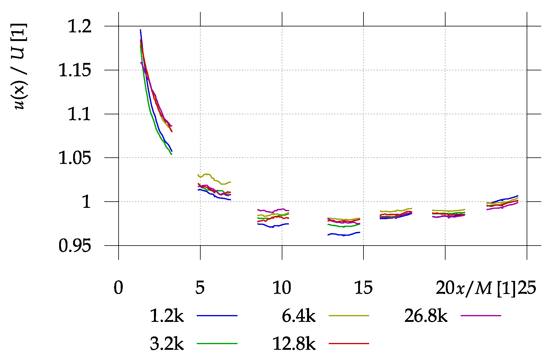
The development of ensemble-averaged stream-wise velocity u is plotted in Figure 4. It is normalized by the average of all ensembles U, which somehow represents the velocity in front of the grid, which is not measured as that area lies inside a metallic part of the wind tunnel without optical access. The average velocity is shown as a function of distance from the grid x normalized by the mesh parameter M. In the near region, the flow field is dominated by the system of wakes and jets, but the measured section cannot be a representative one, as there are not only sections like this (i.e., past the holes and rods oriented perpendicularly), but also sections past the in-plane rods. Therefore, the mass flow in the studied section is larger than the total one containing also sections past rods only. When the pattern of jets and wakes disappears, the velocity corresponds to the total mass flux. However, in later stages, another effect starts to play a role: the boundary layers of the channel slowly grow accelerating the fluid in the center of the channel in order to maintain the total mass flux.
Figure 4.
Ensemble average stream-wise normalized velocity u. The number in the legend is the mesh-based Reynolds number, where k stands for .
3.1. Turbulent Kinetic Energy and Its Decay
Turbulent kinetic energy (TKE) of velocity field is calculated as the energy of fluctuating part
where and are the in-plane velocity components, here u is the stream-wise component, v is one of the span-wise components. Note that true TKE has to be calculated by using all three velocity components, but here we use only the two measured velocity components. Angle brackets denote averaging over time.
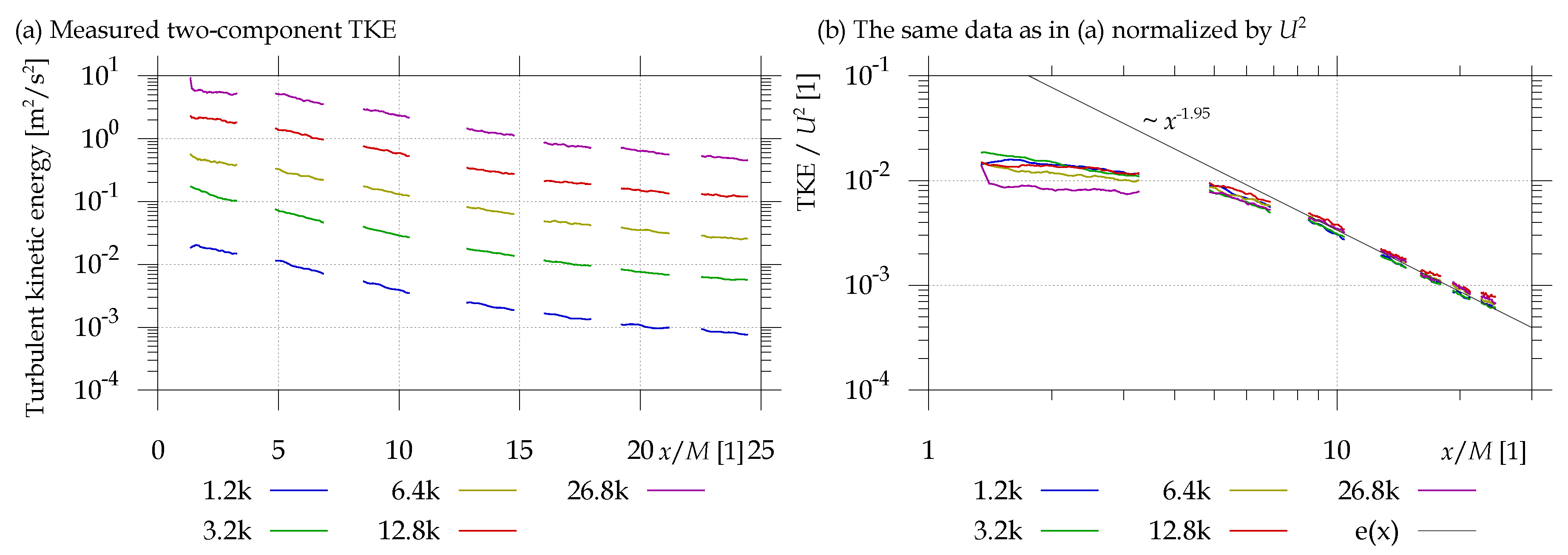
In in Figure 5, the left panel shows the development of turbulent kinetic energy with distance from the grid. Note that the turbulent kinetic energy is calculated only based on the in-plane fluctuations; therefore, it is underestimated by the third component. The number in the legend is the mesh-based Reynolds number, where k plays for . The right panel displays the same data normalized by the average stream-wise velocity U. The function fits the dependence in the far stages. Experimentally, we have found that the turbulent kinetic energy e decays with distance from the grid x as (see black line in Figure 5). Some authors, e.g., [], use a little bit more complicated function with virtual origin ; we prefer to keep the function as simple as possible not introducing too many fitting parameters, because, as John von Neumman said, With four parameters I can fit an elephant, and with five I can make him wiggle his trunk []. In any case, it converges reasonably well within the experimental noise. We can use this function to estimate the energy dissipation rate . The definition of the turbulent kinetic energy dissipation rate is
by using the Taylor hypothesis of frozen turbulence, we can transform it into the x-dependence as
Figure 5.
(a): development of turbulent kinetic energy with distance from the grid. (b): the same data normalized by the average stream-wise velocity U.
Thus, inserting the function from Figure 5 we get
Then, by using the general estimation of the Kolmogorov scale
we can estimate the value of the Kolmogorov length as
with experimentally obtained values of and . The real values of are illustrated in the Table 1 at the position , where the mentioned theory starts to be applicable, and at , where our experimental data end.
Table 1.
Example of Kolmogorov lengths at two positions and for the velocities explored in this experiment.
3.2. Length-Scale Dependent TKE
The effect of vicinity of the Kolmogorov scale to the turbulent kinetic energy is best apparent when we separate turbulent kinetic energy by the length-scale of fluctuations producing it. This is achieved by using the Agrawal decomposition [,], which means the convolution of velocity with band pass filter consisting of two Gauss functions with standard deviations and :
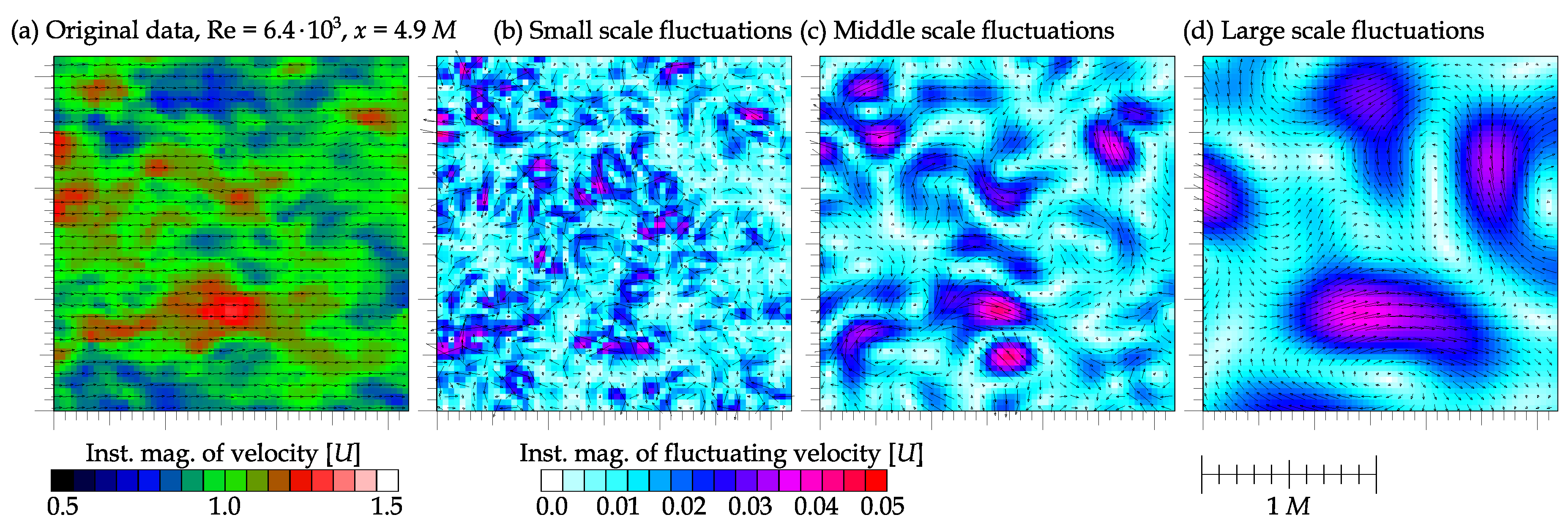
The effect of a such convolution on the velocity field is displayed in Figure 6 for three intervals of length-scales. There is an example of length-scale dependent decomposition also referred as a Agrawal decomposition [,]. A single instantaneous snapshot at and is chosen for this visualization. The scale denoted small corresponds to fluctuations of size or , middle scale means or and the large scale does or . Inst. mag. abbreviates instantaneous magnitude. The velocities are represented in multiples of the mean velocity U.
Figure 6.
Example of length-scale dependent (Agrawal) decomposition.
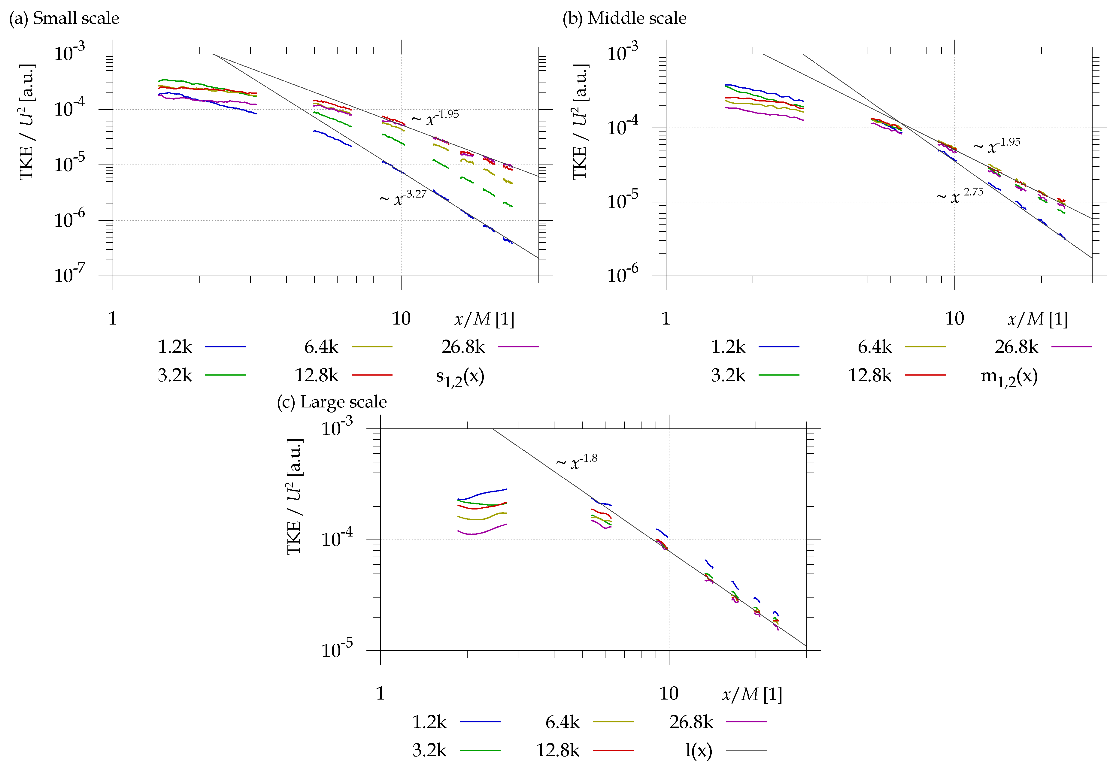
The decay of length-scale dependent TKE is displayed in Figure 7. Turbulent kinetic energies of fluctuations (TKE) of different length-scales are shown, which are visualized in Figure 6. The energy among these scales is not normalized. Therefore, do not compare numbers in these plots, just the shape of curves! Among different velocities, it is normalized by . We can see that the turbulent kinetic energy decays at all scales, but at larger scale, it decays with exponent , while the exponent (previously found in the total TKE, Figure 5) is valid for larger Reynolds numbers at small- and middle- scales. For smallest Reynolds number , the decay is faster with exponent at small scale and at middle scale respectively. We can see, that the decay of TKE at larger Reynolds numbers follow the previously found power law. However, at smaller Reynolds number, it deviates, mainly at small scales (Panel (a) of Figure 7) and it decays significantly faster; therefore, the scaling does not collapse the curves. This effect repeats less strongly at middle scales (Panel (b) of Figure 7), where only the smallest Reynolds number deviates; additionally, the power of faster decay is slightly lower than at small scale. On the other hand, the decay at largest probed scale is slower for all explored velocities. This issue can be physically interpreted as the effect of inverse processes in the Richardson cascade, which pump energy into the larger scales, where it does not originates from the beginning. This partly masks the decay at this largest scale.
Figure 7.
Turbulent kinetic energy (TKE) of different length-scales, (a) small scales, (b) middle scales and (c) large scales.
To see how the length-scale dependent TKE develops, we have to normalize its values among different length-scales by the wavevector length k and the width of the band . Thus, as in the plots of power spectral density we can get the energy content associated with a wavevector k
where is the turbulent kinetic energy of velocity field convoluted with band pass filter of and (Equation (8)), k is the mean wavevector length
and is the width of the wave vector interval
Additionally, we normalize the value of by the famous Kolmogorov scaling , because we consider it a priory, that the turbulence might follow this scaling. Therefore, the normalized of different length scales should collapse in the case of Kolmogorov turbulence.
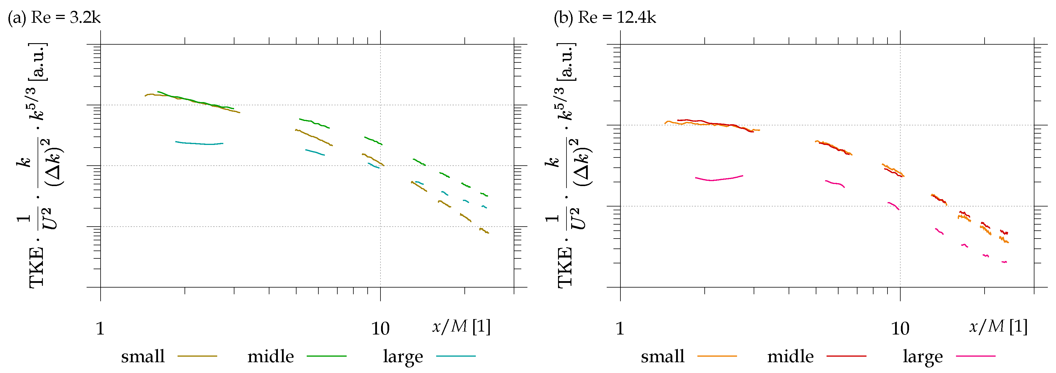
Figure 8 shows such a development of TKE of different length-scales with distance from the grid. Similar to Figure 7 this figure compares the decay of different scale TKE at two selected Reynolds numbers: (a) and (b). The energy is normalized by wavevector length k and the width of the band pass filter , additionally, it is divided by the famous Kolmogorov dependence in order to collapse points, which follow this scaling. This attempt did not succeed; the curves do not collapse even in far regions. It is shown for two velocities only. At the beginning, there is less energy at large scale than that which would correspond to the Kolmogorov scaling, while the middle- and small- scales display intensities comparable within the noise. As the turbulence decays, the energy at all scales decreases, but the large scale TKE decays more slowly approaching the other scales. Within our range of parameters, the curves does not collapse, and thus we pose an interesting question: What happens, when they approach the normalized energy of other scales? (Would they continue decaying with the same power law, or adapt to the decay rate of the other scales?).
Figure 8.
Comparison of the decay of different scale TKE at two selected Reynolds numbers: (a) and (b).
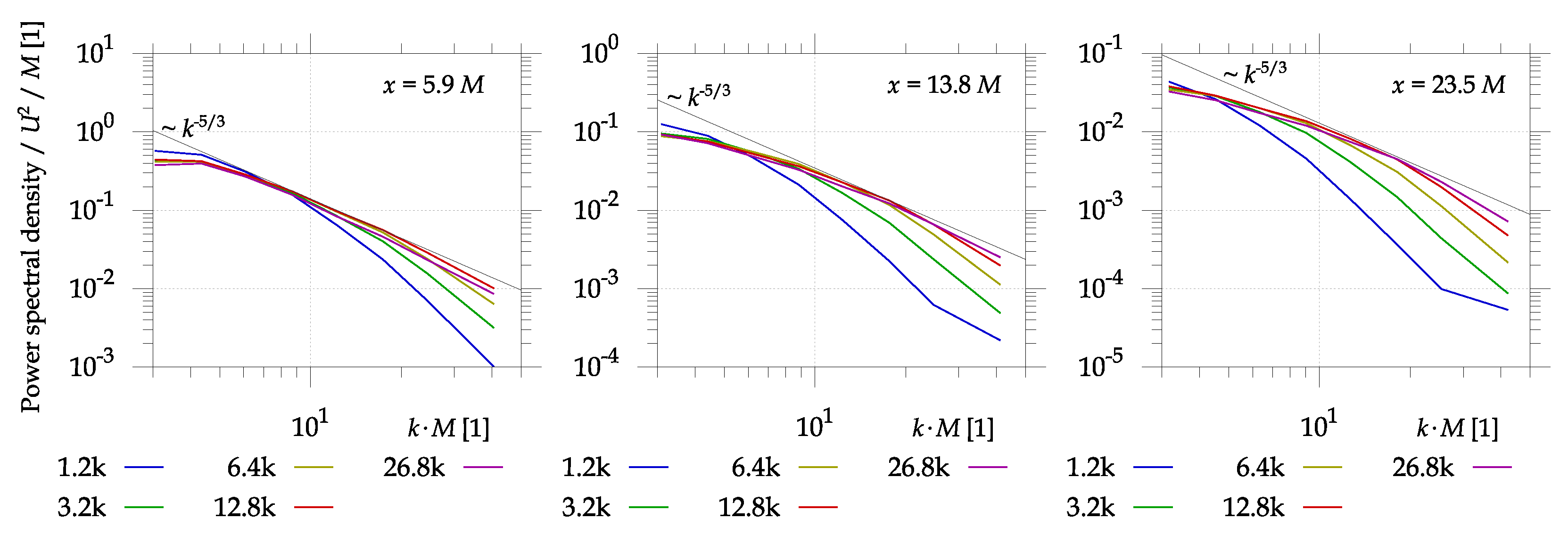
The small scale turbulence decays faster than the middle scale at low Reynolds number, but, at large Reynolds number, it decays in the same way as middle scale turbulence does. This relates to the vicinity of the Kolmogorov dissipative length-scale , which has been estimated in the previous paragraph. In Figure 9, the Spatial power spectral density of turbulent kinetic energy at three distances from the grid: (left), (center) and (right) are shown. The method of spatial spectrum from non-time-resolved data is described in our article []. The is normalized by the velocity square and grid parameter M, wavevector length k is normalized by M. The solid black line represents the Kolmogorov scaling . The spatial spectra in Figure 9 show a similar conclusion: a clear viscosity damping effect at smaller Reynolds numbers visible as a deviation from Kolmogorov scaling depicted in Figure 9 as a solid black line. The method of obtaining a spatial spectrum by using spatially resolved data with poor temporal resolution (note that our equipment allow a maximum sampling frequency only ) as described in detail in our article [] and it is based on the energies of Agrawal decompositions of different bands, as described above.
Figure 9.
Spatial power spectral density of turbulent kinetic energy at three distances from the grid: (left), (center) and (right).
3.3. Vorticity
Vorticity is an important quantity influencing mixing at the small flow scale. Vorticity is defined as rotation of the vector field
The name of this quantity can be a little misleading in referring to vortices. However, vortices are responsible only partly for the vorticity signal []. The second important source is the local shear. The third is the strain rate. Definition (12) is not applicable for experimental data for two main reasons: first, we measure velocities only in a two dimensional section of the 3D flow, therefore, we can calculate only the z component of vorticity; second, we measure at finite resolution. Thus, we approximate partial derivatives in the nabla operator by symmetric differentiation:
where the vector grid resolution and is determined by the experimental setup, not by the Kolmogorov scale, as it should be in ideal case. The measurement of full velocity gradient tensor (and thus determining full vector of vorticity) is possible with a much more complicated setup with a pair of illumination sheets used by Regunath et al. [].
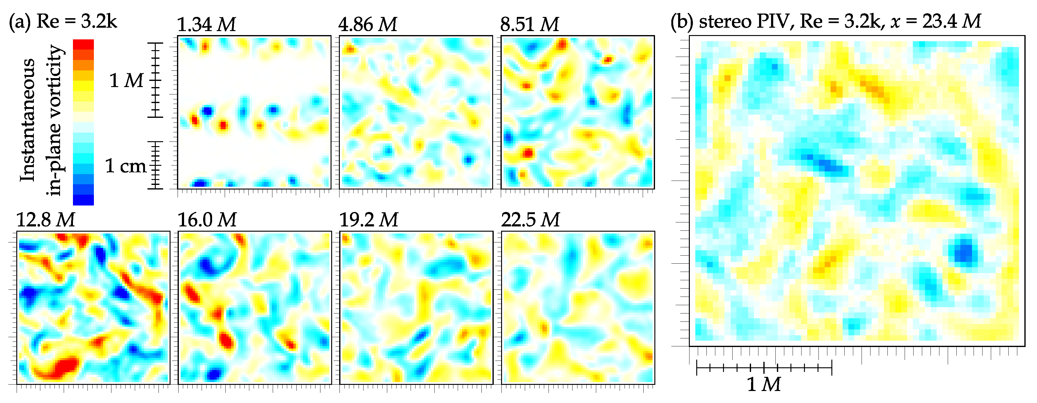
In Figure 10, panel (a), we show an example of instantaneous in-plane vorticity in the 7 studied areas in stream-wise × span-wise direction past the grid at mesh-based Reynolds number . In the top row, the colorscale of vorticity is adapted to that field, while the bottom row, where the vorticity intensity changes not so rapidly, and has a common scale from to . Even by the naked eye we can note the smoothing of structures and (in the bottom row only) the decrease of intensity. In panel (b) of Figure 10, there is an example of instantaneous vorticity obtained by the Stereo PIV technique in a plane perpendicular to the stream-wise direction in distance from the grid . For esthetic purposes, these fields are smoothed by convoluting with Gauss function of grid point. This smoothing is not applied for the plots of statistical moments of vorticity shown later.
Figure 10.
(a) Example of instantaneous in-plane vorticity. (b) Example of instantaneous vorticity obtained by the Stereo PIV technique in a plane perpendicular to the stream-wise direction.
The ensemble average of vorticity has no sense, as it results into ± zero, except in the near-grid region, it may show the shear layers between wakes and jets. More interesting is the standard deviation of vorticity:
The stream-wise dependence of is plotted in Figure 11 as a function of distance . The data are normalized by using the the ratio of distance from the grid x and average stream-wise velocity U, i.e., a time needed to pass there (note the unit of vorticity being , which can be seen as the time needed for turnover). This normalization to a dimensionless quantity does not work as well as for TKE, because it depends on velocity stronger than linearly. This issue can be fixed partially by multiplying by , which is plotted in the right panel. This exponent has been found experimentally and to our knowledge it has no support in the literature. Anyway, the curves still do not collapse. We see that the data at various Reynolds numbers do not collapse. These data collapse little bit better when multiplying by , which is displayed in Figure 11b. In any case, this quantity is much more sensitive to noise, as it is a derivative quantity.
Figure 11.
Normalized standard deviation of in-plane vorticity as a function of distance .
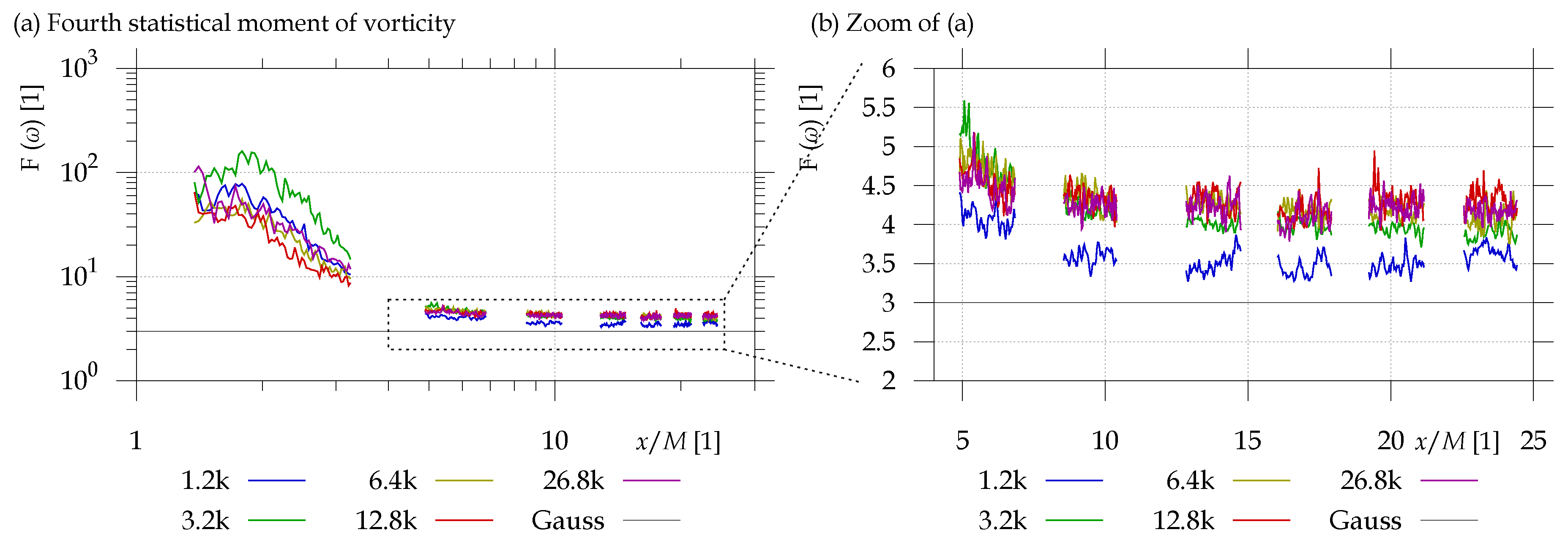
The flatness, i.e., the fourth statistical moment is usually used as a probe of intermittency []. The flatness of Gaussian distribution is calculable analytically and it is equal to 3, which then plays a role of a reference value. High signal means that there is some level of fluctuations (described by standard deviation) disturbed by strong rare events, this behavior is typical for, e.g., neighboring shear layers. The flatness of the vorticity is calculated as
and its stream-wise development is shown in Figure 12 as a function of distance . The flatness of Gaussian distribution is equal to three, which is depicted by the grey line. Flatness larger than 3 signifies appearance of stronger events and large flatness is typical for intermittent effects, which can be found on the edges of shear layers, where the flow is generally quiet, but from time-to-time there comes some turbulent patch; this is the reason for large values of in the near-grid region. In the far region, stays between and with an unprovable weak dependence on Reynolds number. In the near-grid region, the flatness is large, signifying a strong intermittency effect in the pattern of jets and wakes. When we focus to the far-grid region (Figure 12b), we see that the flatness stays between and , which reports the homogeneous appearance of stronger events.
Figure 12.
Flatness of vorticity as a function of distance .
3.4. Isotropy
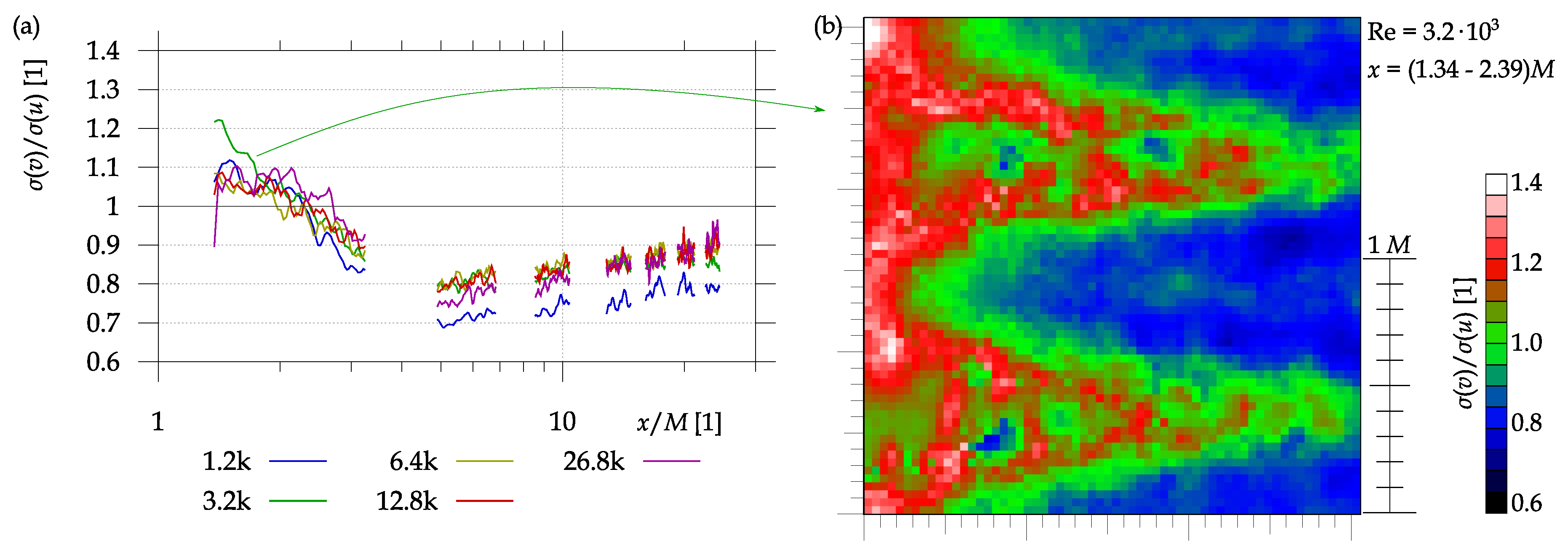
The isotropy, i.e., the independence on the direction, can be best studied by comparing the Reynolds stress tensor components, or its invariants respectively. This can be done only for the stereo PIV data, which we have only at single x. Elsewhere, we can compare at least the ratio of standard deviations of velocity in stream-wise and span-wise directions, []. This is shown in Figure 13 as a function of x. Left panel (a) shows the development of the ratio of fluctuations in span-wise direction () to stream-wise direction () with distance from the grid. The right panel (b) shows one example of the spatial distribution at and at x from to , i.e., in a near grid region, where some spatial distribution related to the shear layers occurs. Green color signifies the same intensity of fluctuations in both investigated directions; red color means prevailing span-wise fluctuations, while blue color shows stronger stream-wise fluctuations. In the near-grid region we see again the effect of regular pattern of jets and wakes.
Figure 13.
(a) development of the ratio of fluctuations in span-wise to stream-wise directions with distance from the grid. (b) example of the spatial distribution at and at x from to .
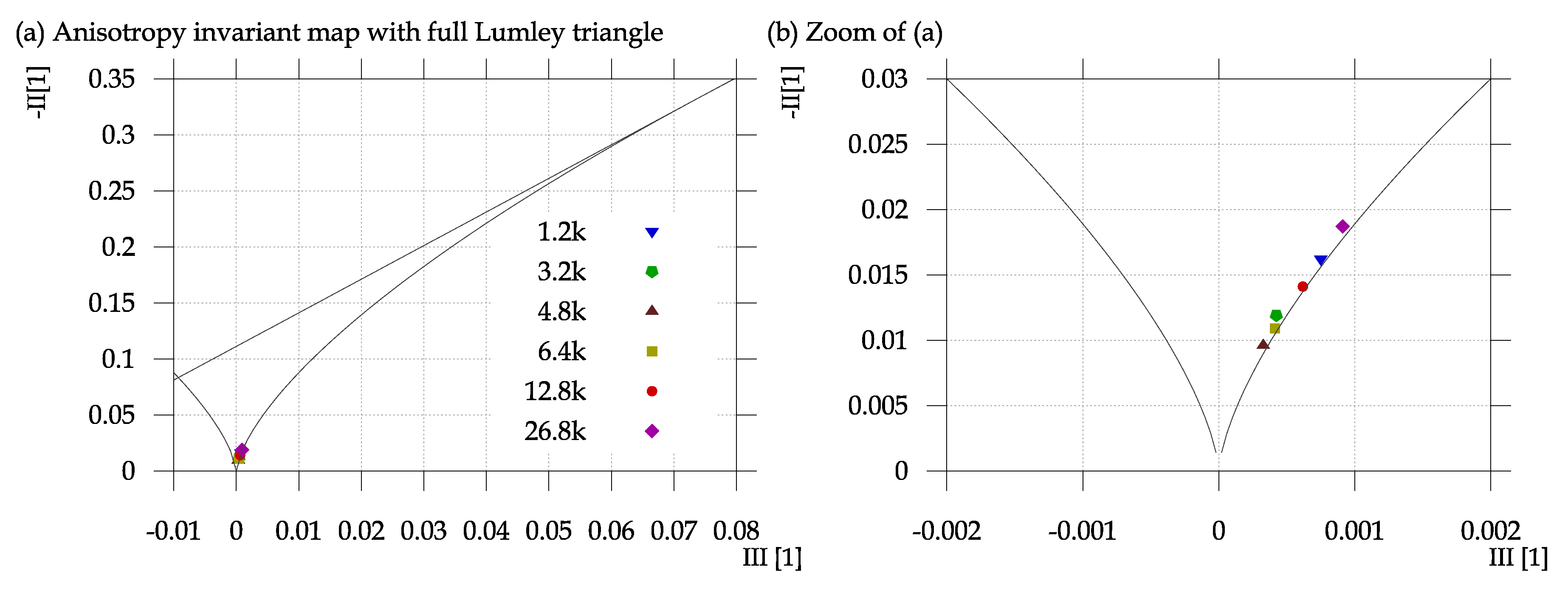
In the case of Stereo PIV we have got all three velocity components in a two-dimensional field; therefore, we can determine the full Reynolds stress tensor . This tensor can be analyzed in the light of its invariants [,,].
Jovanovič [] claims that the anisotropy could be linked to streak patterns appearance in the flow. Those patterns are responsible for primary instability of the flow representing the first stage of turbulence development. The final stage of the fully turbulent flow tends to isotropy (the origin in the AIM graph). The streak patterns are statistically axisymmetric and correspond to a system which is invariant under rotation about the streamwise axis. The sudden appearance of small-scale random motion implies that rapid decrease in anisotropy provokes heavy growth of the dissipation which significantly reduces the smallest scale of motion defined by Kolmogorov’s length-scale. In this way, an energy cascade is initiated, which promotes the spectral separation. This is the essential feature of turbulence and determines its mixing properties. Our results confirm the published finding. The mean flow is significantly non-homogeneous close to the grid (it presents periodic features) and the inhomogeneity in the Reynolds stresses persists well downstream. The inhomogeneity observed in the Reynolds stresses at larger distances downstream of the grid is, in essence, the reminiscence of the initial nonhomogeneity of the mean flow because the turbulence production becomes ineffective at mixing the large-scale structures. Thus, any remaining non-homogeneity existing in the flow when the turbulent production becomes negligible is convected with the flow. The space-averaged data showed that turbulence generated by the grid exhibits a relatively high level of anisotropy which, as the distance behind the grid increases, tends toward one-component turbulence before quickly decreasing. Then, it is followed by a perfect axisymmetric expansion, the turbulence shows a prolate spheroid (rod-like) structure during this decay period.
Indeed, we see that in the far-grid region, there prevail fluctuations in stream-wise direction over those in span-wise one.
The anisotropy coefficient analysis is based on the Reynolds stress tensor
whose anisotropic part is normalized by its trace:
The eigenvalues of tensor are the invariants , and , which are consequently [] defined as
The possible values of invariants and are bounded by the lines depicted in Figure 14 []. Figure 14 shows the spatial average of the values of those invariant over the field of view. The anisotropy invariant map is shown in the coordinates of minus second (-II) and third (III) invariant of the Reynolds stress tensor . These invariants can be calculated only for 3D velocity data, which are obtained by using the Streo PIV, which has been measured at a fixed distance . The so-called Lumley triangle [] of mathematically accessible values is bounded by black lines. The bottom corner at coordinates signifies full isotropy—i.e., fluctuation intensity same in all directions. In the top right corner, there would be turbulence with fluctuations in one direction only, while the left corner is associated with 2D turbulence, see [] for more details.
Figure 14.
Anisotropy invariant map.
The level of isotropy is represented by another parameter F
whose dependence on Reynolds number at the distance is plotted in Figure 15. The errorbars represent the standard deviation of this property within the field of view. We see that the flow is almost isotropic ( [,]) according to this parameter and an interesting behavior is that it has a maximum at finite Reynolds number . The reason of anisotropy could be appearance of streaky structures. The character of increasing and later decreasing value of F is unknown for us at this moment, but note that it might be an artifact of the PIV method, which is unable to resolve too small turbulent scales (and Reynolds number is closely related to the ratio of smallest to largest scale).
Figure 15.
Anisotropy coefficient F as a function of Reynolds number at distance .
4. Conclusions
We manufactured a regular grid of square rods by a 3D printer. By means of 3D optical scanning, we found that the grid is neither as regular or as square as we planned. We venture to believe that other studies also suffer from this deviation between the planed and the actual geometry, although it is usually not reported. The grid geometry forms the boundary condition for the flow, so it is of high importance to be defined as precisely as possible.
We measured the flow velocity past the grid by using a commercially available PIV (Particle Image Velocimetry) system. We focus our analysis to the decay rate of turbulent kinetic energy and we found the decay exponent of for all Reynolds numbers from to . In classical literature, a smaller absolute value of this exponent is reported very often. Comte-Bellot and Corrsin [] found this exponent within the range and , Warhaft and Lumley [] estimated the exponent , to mention just a few. However some other authors dealing with similar grid geometry as used in our case (e.g., [,] evaluated this coefficient in broader range from up to ).
The most important results presented in the paper deal with evaluation of TKE connected with various fluctuation scales. For this purpose we have decomposed the turbulent velocity field into three parts according to coherent structure scales by means of the Agrawal decomposition method []. The obtained small scale, middle scale and large scale turbulent contents were analyzed separately. The decay laws were evaluated for each component. Gentle decay was found for the large scales, the exponent was about only, independent on the Reynolds number. However for the middle and small scales steeper decays were detected characterized by the exponents in range between to . The exponent value applies for high Reynolds numbers, while small Reynolds number shows steeper decay, exponent for small scales and for middle scales. Hence, we could conclude that small scale fluctuations decay faster than the large scales especially at low Reynolds numbers. This effect could be related to the fact that the small scales are approaching the Kolmogorov scale at low Reynolds numbers. At larger Reynolds numbers, the decay rate is close to that of the total TKE. The studied effect has consequences in the turbulence spectrum development in stream-wise direction and mixing properties.
The isotropy is analyzed by using the ratio of standard deviations in stream-wise and span-wise directions. It shows stronger contribution from the stream-wise direction. The analysis of Reynolds stress tensor invariants shows a nearly 3D isotropy of the turbulence weakly shifted towards the 2D isotropy. This result is expected and in accordance with the results reported in the literature (see, e.g., [,]).
The next step in our research will be a deeper analysis of the decomposed turbulent flow-field. Standard analysis methods are to be applied separately on specific turbulent components. In the future we also would like to study the effect of the grid-generator quality on the generated turbulence. We will concentrate on details of its geometry, e.g., curvature of corners, and namely on the grid surface roughness. The mixing properties are to be evaluated and optimized.
Author Contributions
Conceptualization, V.U. and D.D.; methodology, V.U.; software, D.D.; validation, V.Y.; investigation, D.D.; resources, V.Y.; data curation, D.D.; writing–original draft preparation, D.D.; writing–review and editing, V.Y. and V.U.; visualization, D.D.; supervision, V.U. All authors have read and agreed to the published version of the manuscript.
Funding
This work was supported by the Grant Agency of the Czech Republic, project No. 17-01088S.
Acknowledgments
The work was supported from ERDF under project Research Cooperation for Higher Efficiency and Reliability of Blade Machines (LoStr) No. CZ.02.1.01/0.0/0.0/16_026/0008389. We would thank to Petr Eret for help with the 3D scanning and with the above mentioned project.
Conflicts of Interest
The authors declare no conflict of interest.
Abbreviations
The following abbreviations are used in this manuscript:
| PIV | Particle Image Velocimetry |
| TKE, e | Turbulent kinetic energy based on the 2D velocity data, |
| Re, | Mesh-based Reynolds number, |
| u, v | stream-wise and span-wise velocity components |
| k | length of the wavevector, unit is inverse millimeter, |
| M | Mesh parameter of the grid, in this experiment |
| d | Size of the grid rod, in this experiment |
Appendix A. Discussion the TKE Calculation Method
We calculated the turbulent kinetic energy by using the two measured velocity components, see Equation (2). This way underestimates the result, as the contribution from the third velocity component is missing (and it is always a positive number). Some authors solve this issue by incorporating the second (span-wise) velocity component twice:
The argument stays, that due to symmetry, the invisible component may fluctuate with same intensity, thus we can estimate the real value better. We prefer to not use any a priory consideration about the symmetry or isotropy of the flow, even when the isotropy level is a subject of research. However, the TKE manipulated in this way is closer to the values obtained by using all three velocity components, which is possible with the Stereo PIV setup. Figure A1 shows the comparison at , where the Stereo PIV data are acquired. There is the comparison of TKE measured by using the classical PIV with 2 velocity components (blue down triangles) and that measured by using Stereo PIV returning three velocity components (brown up triangles). The red circles represent the TKE calculated from the 2D data with contributing the span-wise velocity component twice. Panel (a) shows the measured value in , while panel (b) shows the value normalized by average stream-wise velocity.
The evaluated TKE is used in the paper for determination either decay law or to compare energy content of various scales. Thus we insist on the first definition of the TKE, as only relative changes are relevant and not the TKE absolute value.
Figure A1.
Comparison of TKE measured by using the classical PIV with 2 velocity components (blue down triangles) and that measured by using Stereo PIV returning three velocity components (brown up triangles). (a) shows the measured values, while in (b), the values are normalized by the velocity in order to see the difference.
References
- Pope, S.B. Turbulent Flows; Cambridge University Press: Cambridge, UK, 2000; p. 771. [Google Scholar]
- Roach, P. The generation of nearly isotropic turbulence by means of grids. Int. J. Heat Fluid Flow 1987, 8, 82–92. [Google Scholar] [CrossRef]
- Kolmogorov, A.N. Dissipation of Energy in the Locally Isotropic Turbulence. Proc. R. Soc. A Math. Phys. Eng. Sci. 1991, 434, 15–17. [Google Scholar] [CrossRef]
- Bourgoin, M.; Baudet, C.; Kharche, S.; Mordant, N.; Vandenberghe, T.; Sumbekova, S.; Stelzenmuller, N.; Aliseda, A.; Gibert, M.; Roche, P.; et al. Investigation of the small-scale statistics of turbulence in the Modane S1MA wind tunnel. CEAS Aeronaut. J. 2018, 9, 269–281. [Google Scholar] [CrossRef]
- Machado, F.; Malpica, N.; Borromeo, S. Parametric CAD modeling for open source scientific hardware: Comparing OpenSCAD and FreeCAD Python scripts. PLoS ONE 2019, 14. [Google Scholar] [CrossRef]
- Inkinen, S.; Hakkarainen, M.; Albertsson, A.; Södergøard, A. From lactic acid to poly(lactic acid) (PLA): Characterization and analysis of PLA and Its precursors. Biomacromolecules 2011, 12, 523–532. [Google Scholar] [CrossRef] [PubMed]
- Tropea, C.; Yarin, A.; Foss, J.F. Springer Handbook of Experimental Fluid Mechanics; Springer: Heidelberg, Germany, 2007; p. 1557. [Google Scholar]
- Duda, D.; Uruba, V. Spatial Spectrum From Particle Image Velocimetry Data. ASME J. Nucl. Rad Sci. 2019, 5. [Google Scholar] [CrossRef]
- Mohamed, M.; LaRue, J. The decay power law in grid-generated turbulence. J. Fluid Mech. 1990, 219, 195–214. [Google Scholar] [CrossRef]
- Meyer, J.; Khairy, K.; Howard, J. Drawing an elephant with four complex parameters. Am. J. Phys. 2010, 78, 648–649. [Google Scholar] [CrossRef]
- Agrawal, A.; Prasad, A. Properties of vortices in the self-similar turbulent jet. Exp. Fluids 2002, 33, 565–577. [Google Scholar] [CrossRef]
- Agrawal, A. Measurement of spectrum with particle image velocimetry. Exp. Fluids 2005, 39, 836–840. [Google Scholar] [CrossRef]
- Kolář, V. Vortex identification: New requirements and limitations. Int. J. Heat Fluid Flow 2007, 28, 638–652. [Google Scholar] [CrossRef]
- Regunath, G.S.; Zimmerman, W.B.; Tesař, V.; Hewakandamby, B.N. Experimental investigation of helicity in turbulent swirling jet using dual-plane dye laser PIV technique. Exp. Fluids 2008, 45, 973–986. [Google Scholar] [CrossRef]
- Tabeling, P.; Zocchi, G.; Belin, F.; Maurer, J.; Willaime, H. Probability density functions, skewness, and flatness in large Reynolds number turbulence. Phys. Rev. E 1996, 53, 1613–1621. [Google Scholar] [CrossRef]
- Romano, G. Large and small scales in a turbulent orifice round jet: Reynolds number effects and departures from isotropy. Int. J. Heat Fluid Flow 2020, 83, 108571. [Google Scholar] [CrossRef]
- Lumley, J.L.; Newman, G. The return to isotropy of homogeneous turbulence. J. Fluid Meach. 1977, 82, 161–178. [Google Scholar] [CrossRef]
- Simonsen, A.J.; Krogstad, P.O. Turbulent stress invariant analysis: Clarification of existing terminology. Phys. Fluids 2005, 17, 088103. [Google Scholar] [CrossRef]
- Choi, K.; Lumley, J.L. The return to isotropy of homogeneous turbulence. J. Fluid Meach. 2001, 436, 59–84. [Google Scholar] [CrossRef]
- Jovanovic, J.R.; Nishi, M. The Origin of Turbulence in Wall-Bounded Flows. Therm. Sci. 2017, 21, S565–S572. [Google Scholar] [CrossRef]
- Uruba, V. (An)isotropy analysis of turbulence. In Proceedings Topical Problems of Fluid Mechanics; Šimurda, D., Bodnár, T., Eds.; Institute of Thermomechanics: Prague, Czech Republic, 2015; pp. 237–244. [Google Scholar]
- Uruba, V. Decomposition methods for a PIV data analysis with application to a boundary layer separation dynamics. Trans. VŠB Tech. Univ. Ostrav. Mech. Ser. 2010, 56, 157–162. [Google Scholar]
- Comte-Bellot, G.; Corrsin, S. The use of a contraction to improve the isotropy of grid-generated turbulence. J. Fluid Mech. 1966, 25, 657–682. [Google Scholar] [CrossRef]
- Warhaft, Z.; Lumley, J.L. An experimental study of the decay of temperature fluctuations in grid generated turbulence. J. Fluid Mech. 1978, 88, 659–684. [Google Scholar] [CrossRef]
- Jonáš, P.; Mazur, O.; Uruba, V. On the receptivity of the by-pass transition to the length scale of the outer stream turbulence. Eur. J. Mech. B/Fluids 2000, 19, 707–722. [Google Scholar] [CrossRef]
- Grzelak J., W.Z. The decay power law in turbulence. Trans. Inst. Fluid Flow Mach. 2015, 130, 93–107. [Google Scholar]
- Kurian, T.; Fransson, J.H.M. Grid-generated turbulence revisited. Fluid Dyn. Res. 2009, 41, 021403. [Google Scholar] [CrossRef]
Publisher’s Note: MDPI stays neutral with regard to jurisdictional claims in published maps and institutional affiliations. |
© 2020 by the authors. Licensee MDPI, Basel, Switzerland. This article is an open access article distributed under the terms and conditions of the Creative Commons Attribution (CC BY) license (http://creativecommons.org/licenses/by/4.0/).