Abstract
Owing to the pollution free nature, higher efficiency and noise free operation, fuel cells have been identified as ideal energy sources for the future. To avoid direct storage of hydrogen due to safety considerations, storing hydrocarbon fuel such as methane and suitably reforming in situ for hydrogen production offers merit for further investigation. Separating the resulting hydrogen in the reformate using membrane separation can directly feed pure gas to the anode side of fuel cell for power generation. Despite the numerous works reported in literature on the dynamic and steady state modeling and analysis of reformers, membrane separation units and fuel cell systems, there has been limited work on an analysis of the integrated system consisting of all the three components. This study focuses on the mathematical modeling and analysis of the integrated reformer, membrane, fuel cell system from first principles in a dynamic framework. A multi loop control strategy is developed and implemented on the mathematical model of the integrated system in which appropriate controllers based on the system dynamics are designed to examine and study the overall closed loop performance to achieve rapidly fluctuating target power demand and rejection of reformer feed and fuel cell coolant temperature disturbances.
1. Introduction
The main focus of emergent hydrogen economy for the last few decades has been on the use of hydrogen fuel cells for stationary and portable applications. Almost all practical fuel cells available in the current market use hydrogen or hydrogen-rich hydrocarbons as the fuel [1]. While designing a fuel cell system, the primary challenge of a systems engineer is to make sure that the desired quantity of fuel is delivered at the appropriate time. In the case of fuel cells driven by hydrogen, the prevailing method to deliver hydrogen entails storing of the fuel in appropriately designed high pressure tanks that can withstand high pressures of the order of 350 to 700 bars [1]. Large volume vessels are generally needed for hydrogen storage because of its low volumetric energy density [1]. For automotive applications, while this demanding requirement of large volume might have a lesser impact on heavy duty vehicles, it can be a crucial issue for light duty vehicles. A key issue for portable applications is the non-availability of hydrogen fueling infrastructure for refueling purposes. Furthermore, hydrogen when exposed to air can easily catch fire and can lead to explosion thereby underlining the high risk of direct hydrogen storage. The need to avoid direct storage of hydrogen triggered the development of integrated fuel processing system that converts hydrogen rich hydrocarbons directly to a hydrogen fuel stream. It is well known that hydrogen production by reforming natural gas is an economically viable alternative since infrastructure for natural gas supply already exists.
In the current work, an auto thermal reformer that incorporates both endothermic steam reforming and exothermic partial oxidation is used. Hence, the hydrocarbon fuel viz. natural gas reacts with oxygen from air and steam over a catalyst in a fixed bed reactor at suitable operating conditions to obtain appropriate hydrogen yield along with other gases such as , , , unconverted , (steam) and the inert [2]. The advantage of auto thermal reforming over steam reforming include self-sustained reaction by using the heat generated by the combustion reaction for the prevalent endothermic reactions. Among the methods for separation of gases at the reformer exit, dense palladium membrane has been employed in the current work for separation of from mixture of other gases [3]. Palladium membranes have the advantage of high hydrogen permeability as well as fast hydrogen absorption and transport kinetics. Another advantage is its excellent thermal stability at an operating temperature range of 300–850 C [4]. These behaviors are important from a rapid dynamic response viewpoint when used in an integrated system. Finally, a low temperature polymer electrolyte membrane fuel cell (PEMFC) is used for electrical power generation that occurs in response to the electrochemical reaction of hydrogen and air as source of oxygen.
To overcome the deficiencies of direct hydrogen storage, this work explores the potential of an integrated natural gas reformer fuel cell system with membrane-based gas separation/purification using the dynamic models for each. The frequency of start/stop cycles as well as the weight and size of the integrated system are a few of the vital factors to be considered while designing the power supply system [5]. While significant works have been carried out on the dynamic behavior of the individual subsystems viz. reformer, membrane and fuel cell, only a handful of them have directed their research on integration of these subunits [5,6]. The integration of the downstream fuel cell system with the upstream fuel processing system poses several challenges from a dynamics and control viewpoint. Firstly, the response time of a fuel cell is at least an order of magnitude faster than the fuel processing system (auto thermal reformer). Also, the variation in power demands, depending on the duty cycle of the electrical load in the application, needs to be adhered by the fuel cell and this should trigger appropriate decisions at the reformer level. Secondly, due to slow reformer dynamics, lead-like behavior in control mechanisms could be anticipated. Also, the integrated system needs to accommodate line-pack associated aspects for hydrogen. Hence, in this work, we focus on examining the feasibility of the integrated reformer fuel cell system with a membrane separation unit for power applications. Use of hydrocarbon fuels with solid oxide fuel cell via internal reforming have been reported [7,8]. In Ref [9], syngas has been used with molten carbonate fuel cell for power generation. Hydrocarbon as the primary source of hydrogen in PEMFC is challenging since PEMFC cannot tolerate impurities. The authors in Ref [6] discuss a detailed design and control framework of a bio-ethanol steam reformer integrated with PEMFC using Aspen HYSYS simulation software. Protection of the fuel cell stack due to hydrogen/oxygen starvation, higher system efficiency (i.e., maximum ethanol to hydrogen conversion) were a few of the objectives considered by the authors while designing the controllers. The authors in Ref [5] investigated and compared high temperature and low temperature PEMFCs with different fuel processors using glycerol as the fuel. Ref [10] examined the dynamic electrochemical model of a PEMFC along with a methanol reformer and a power conditioning unit. This latter work used a simplified transfer function-based fuel cell model and did not discuss the possibility of integration of the units. Out of the very few works on the integrated reformer fuel cell system reported in the literature, Ref [11,12] explored the dynamic system interaction using liquid methanol as the fuel. However the authors did not consider separation of the hydrogen gas exiting from the reformer output.
The main contribution of this paper is exploring the integrated reformer membrane fuel cell system for dynamic performance under realistic scenarios. An appropriate control structure is designed based on four single loop controllers for overall system operation. The integrated system is evaluated for tracking the target power profile for a representative power application as well as disturbance rejection. The results show the potential of the integrated system for power generation applications and highlight the need for auxiliary power supply during cold startup of the reformer.
The rest of the paper is organized as follows. A brief description of the fuel processing, fuel purification, power generation subsystems as well as the overall integrated system along with its mathematical modeling are discussed in the next Section. In Section 3, we present three case studies: the first being an open loop simulation for start-up of the integrated reformer membrane fuel cell system. Subsequently, the relative gain array analysis is presented to choose the input-output pairings for carrying out control relevant studies. The second case study involves the integrated system used for a generic power application with suitably designed controllers and the final case study evaluates disturbance rejection by considering uncertainty in both the inlet feed concentration to the reformer as well as coolant temperature in fuel cell. This is followed by simulation results and discussions. Conclusions are presented in Section 4.
2. System Description
To understand the behavior of the integrated reformer membrane fuel cell system as a whole, detailed dynamic modeling of the individual subsystems is necessary. This will help identify possible challenges for achieving smooth, demand-driven production and delay-free delivery of hydrogen fuel [6]. The basic block diagram showing the integrated system is depicted in Figure 1. The input to the auto thermal reformer consists of appropriate proportion of methane, air and steam thoroughly mixed and preheated to reforming temperatures during start of the reaction. Once the reactions are initiated, the preheater can be removed from the loop as the heat liberated by the exothermic reactions can be further used by the endothermic reactions. The reforming reaction of methane with air and steam results in products such as , and along with some unreacted , , and steam. Two heat exchangers, one at the reformer exit and other at the fuel cell anode inlet side, are used to maintain the gas temperatures at their target values and is assumed to be under perfect control. The gas mixture exiting the reformer is then separated to obtain pure hydrogen by using the palladium membrane based separation unit. The pure hydrogen gas separated from the gas mixtures is then fed to the control valve 2 inlet through a check valve or non-return valve (NRV). The hydrogen is then used by the fuel cell to generate power. Four controllers, one to regulate hydrogen flow at the fuel cell anode inlet side, second to regulate methane flow at the reformer inlet side, third to regulate the coolant flow at the PEMFC coolant circulation side and fourth to regulate the ratio of air to in PEMFC are implemented to achieve effective operation of the integrated system. The three major components namely, fuel processing subsystem, fuel purification subsystem and power generation subsystem are discussed in detail in the subsequent sections.
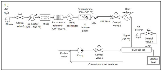
Figure 1.
Block diagram showing the integrated reformer membrane fuel cell system. (NRV: non-return valve; PEM: polymer electrolyte membrane).
2.1. Fuel Processing Subsystem: Auto Thermal Reformer
An auto thermal reformer employing methane as the fuel is chosen as the fuel processing subsystem in the current study. The upstream part of the reactor is dominated by the highly exothermic oxidation reaction whereas endothermic steam reforming reactions dominates the downstream part. A feed stream consisting of steam to carbon molar ratio of 1:1 and oxygen to carbon molar ratio of 0.45:1 is considered. Many reactions such as steam reforming, water gas shift, total combustion, partial oxidation, partial combustion, dry reforming, boudouard reaction and decomposition reaction are likely to occur in an auto thermal reformer [2]. Among this possible set of reactions, only the dominant reactions with significant rates are considered in this study in order to reduce the complexity of the mathematical model. Reactions in Equations (1) and (2) represent the steam reforming reactions while Equations (3) and (4) represent the water gas shift and total combustion reactions respectively [2].
Mathematical Model of Auto Thermal Reformer
Auto thermal reforming has been widely studied and experimental validation has been reported in the literature [2,13,14,15]. The authors in [13] performed a steady state analysis of hydrogen production from methane using an auto thermal reformer with a dual catalyst bed configuration, but did not discuss the dynamic behavior of the system. Extensive experiments were conducted on an in-house developed auto thermal reformer by the authors in [14] and the experimental results were used to validate the mathematical model developed. Ref [15] analyzed the steady state modeling aspects of a miniaturized methanol reformer for fuel cell powered mobile applications but did not study the dynamic behavior of the system. In this work, a one-dimensional dynamic model of the auto thermal reformer is selected [2]. Energy and mass balances are applied both in gas and solid phases to obtain the mathematical model of the reformer. The reformer consists of a cylindrical reactor of 0.2 m in length and with Nickel as the catalyst having a density of 1870 kg m. Both the gas feed as well as catalyst temperature is maintained at a value of 542 C. The reformer operating pressure is chosen to be 1.5 atm with a Gas Hourly Space Velocity (GHSV) of 3071 h implying a residence time of 1.17 s and a gas mass flow velocity of 0.15 kg m s−1. The schematic showing the flow diagram of the modeled region in an auto thermal reformer is shown in Figure 2. The auto thermal reformer model involves seven main species (, , , , , ) including one inert component ( from air). For more particulars on the operating conditions, kinetic parameters, constants, kinetic reaction model and gas properties examined in the model, the reader is referred to Ref [2].
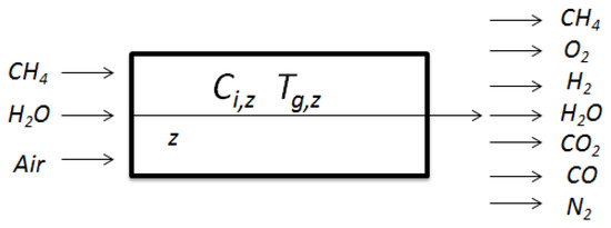
Figure 2.
Flow diagram of modeled region in an auto thermal reformer.
While modeling the reformer subsystem, it is assumed that the gas behavior is ideal and the reforming operation is adiabatic in nature. Thermal dispersion in the axial direction is modeled and negligible radial gradients are assumed. Temperature gradient in the catalyst particles is also ignored assuming the particle size and bed porosity to be uniform.
Mass balance for each species in the gas phase is given by:
Mass balance for the solid phase is given by:
The first term on the left hand side of Equation (5) represents the mass accumulation term of each component while the second term indicates convective diffusion. Mass transfer from gas to solid is represented by the third term and is evaluated using Equation (6). The term on the right hand side of Equation (5) gives the axial dispersion of components.
Energy balance on the gas phase is given by:
The first term on the left hand side of Equation (7) represents the heat accumulation term while the second term indicates convective heat transfer. The first term on the right hand side represents the heat transfer from gas to solid and the second term indicates the conductive heat transfer.
Energy balance on the solid phase is given by:
The term on the right hand side of Equation (8) involves the heat of reaction term multiplied by the catalyst density and packed bed porosity.
The pressure drop across the reformer bed is given by Ergun equation and can be expressed as:
Boundary Conditions are as follows:
Initial conditions are as follows:
2.2. Fuel Purification Subsystem: Palladium Based Membrane Separation
Efficient operation of a low temperature PEMFC inevitably demands purified hydrogen gas at the anode inlet. The efficiency and lifetime of the fuel cell strongly depends on the rate of poisoning of the catalyst due to the presence of impurities in the feed. Palladium alloy-based membrane separation is reported to be an attractive method for the purification of hydrogen gas from mixture of other gases [16]. Another alternative method for hydrogen gas purification is the pressure swing adsorption (PSA) that works according to the species molecular characteristics and affinity for an adsorbent material [17,18]. However due to size constraints, this method may not be suitable for portable applications and hence not considered for this particular study. The authors in [19] has developed a mathematical model of the palladium-based membrane separation for hydrogen gas separation and has experimentally validated the model. Irrespective of whether the separation is required for portable or stationary applications, palladium-based membrane separation can be efficiently exploited for the gas purification process. Palladium membrane has the added advantage of having low permeability for other gases compared to hydrogen gas which effectively qualifies it for gas separation/purification [3,4].
Mathematical Model of Palladium Membrane Separation
According to Sievert’s law [16], permeation of gas occurs through the palladium membrane based on the difference in partial pressures of hydrogen at both sides of the membrane. The molar flow rate of hydrogen permeating through the palladium membrane according to Sievert’s law is given by [16]
Variable stands for the membrane poisoning caused by the adsorption of on the membrane surface which can partially prevent or obstruct the hydrogen permeation and () denotes the fraction of membrane actually available for the hydrogen gas separation. The membrane permeability is a function of temperature which can be represented by the Arrhenius law as
where , , R and represents permeability pre-exponential factor, activation energy for hydrogen permeability, gas constant and gas temperature at the exit of heat exchanger 1 respectively. More hydrogen crossover can be facilitated than the predicted behavior by the Sievert’s law due to the presence of defects in the membrane layers. However, due to this, other gas species can also pass across the membrane allowing the overall flux to be the sum of hydrogen flux given by Sievert’s law and the flux of other gases through the defects. This aspect has not been pursued in the present work.
2.3. Power Generation Subsystem: PEMFC
Hydrogen gas exiting from the fuel processing subsystem after undergoing necessary purification is fed to the anode side of the PEMFC to generate electricity. Using a blower, air from the atmosphere is fed to the cathode side of the PEMFC. In this study, hydrogen is considered to be the limiting reagent while air is considered as the excess reagent. Although the stoichiometric ratio of the inlet molar flow rate of hydrogen to oxygen is 2, the molar flow rate of air is chosen to be always 5 times greater than the molar flow rate of hydrogen fed to the fuel cell. This is achieved by employing a ratio controller that senses the flow rate of hydrogen and adjusts the control valve 4 position to allow requisite flow of air to enter the fuel cell cathode. As soon as the reactants are directed to the active catalyst sites through the fuel cell electrodes, electrochemical reactions initiate and load current is generated. The electrochemical reactions that occur in a PEMFC are shown in Table 1. A single cell has an open circuit voltage of around 1 V and under load, it drops down to 0.6 to 0.7 V. Real world applications demand electricity of the order of several tens or hundreds of volts. To achieve these high voltage values, individual fuel cells are stacked in series so that the aggregate voltage fits any specified voltage requirement. To maintain acceptable conductivity, the polymer membrane requires to be hydrated with water. For achieving this, the fuel cell must operate at temperatures below 90 C.

Table 1.
Electrochemical reactions in PEMFC (PEMFC: polymer electrolyte membrane fuel cell).
Mathematical Model of PEMFC
Numerous studies in fuel cell dynamics have been reported in the literature [5,20,21]. The study of the dynamic operation of a fuel cell is crucial for both portable and stationary applications, where power demand varies, and the fuel cell does not generally operate at the designed optimal steady-state [20]. Considerable amount of work using fuel cell system dynamics have been reported in which authors in Ref [5] studied the case of a high temperature PEMFC with and without a water gas shift reactor used for carbon monoxide removal. In Ref [21], the dynamics of the fuel cell using an air compressor as source for oxygen/air has been studied by assuming direct storage of hydrogen. The model equations for PEMFC considered in this paper involves an along the channel model adopted from Ref [20]. The schematic showing the flow diagram of the modeled region in a PEMFC is shown in Figure 3 [22]. The mathematical model includes set of ordinary differential equations comprising of consumption equations for each species ( at the anode and air at the cathode), balance of water and temperature of gas at both the anode and cathode side as well as the coolant temperature. The temperature variation of the polymer membrane consists of a partial differential equation while the Nernst equation, which is an algebraic equation, describes the voltage obtained from the PEMFC.
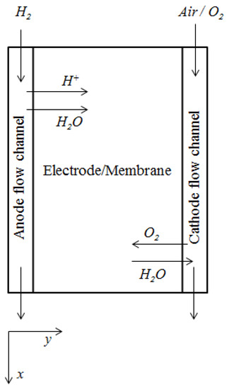
Figure 3.
Flow diagram of modeled region in a PEMFC (PEMFC: polymer electrolyte membrane fuel cell) [22].
For more details on the amount of water molecules transported by each proton, membrane conductivity, various assumptions and parameter values used in the model, the reader is referred to the references [20,23]. Apart from the energy balance equation, all the remaining equations are considered to be at quasi steady state.
Equations for consumption of a single phase species i along the channel length is given by
where,
Balance of water in liquid form is influenced by the effect of evaporation and condensation which is given by
It is significant to note that Equation (17) is used only when liquid water exists at the anode or cathode and/or partial pressure of water in vapour form exceeds its saturation pressure.
At the anode side, equation for water vapor balance is given by
The first term on the right hand side of Equation (18) represents the evaporation/condensation rate of liquid water while the second term indicates the net amount of water migrated across the membrane.
At the cathode side, equation for water vapor balance is given by
The electrochemical reaction at the cathode side of the fuel cell generates some amount of water vapor and is represented by the last term of Equation (19). Appropriate heat removal and humidification are essential for the membrane to be suitably hydrated and conductive which in turn lowers the ohmic losses in the cell. The humidification of membrane is characterised by the term alpha () given by Equation (20) which denotes the ratio of water molecules per proton. Equations (18) and (19) contain the term which indicates the net amount of water migrated across the polymer membrane. Equation (21) indicates the effect of humidity or water content on the conductivity of the membrane. Reduction in membrane humidity can in turn reduce the membrane conductivity and can further cause a reduction in the cell voltage (see Equation (31)). The ratio of water molecules per proton, , is expressed as
The expression for conductivity of the membrane is given as
The expressions for and are given by
The activities of water in the anode and cathode are defined as,
The equation for the variation in anode and cathode gas temperatures are given by
The variation in temperature of coolant circulated is expressed as
The spatial and time dependency of solid temperature is determined by the energy balance equation given by
The first term on the right hand side of Equation (28) represents the heat transfer by conduction, second term indicates the heat transfer to the fuel and oxidant flows, third term gives the heat transfer to the coolant channels, fourth term represents the heat generation by the reactions and the last term indicates the heat of evaporation/condensation.
The boundary conditions given by Equation (29) indicates the heat energy lost to the surroundings from both the edges of the membrane by convection.
The cell voltage attained from the PEMFC given by the Nernst equation is expressed as
The overall output voltage obtained from the PEMFC considering the losses is given by
The third term of Equation (31) represents the activation over potential and last term represents the ohmic over potential. Concentration over potential is not taken into account in this particular mathematical model.
2.4. Integrated Reformer Membrane Fuel Cell System
The integrated system essentially comprises of a combination of the three subsystems viz. reformer, membrane and fuel cell to form a single unit. Present work discusses the detailed mathematical modeling and control studies of the integrated system with a multi-loop control strategy along with a few case studies. As can be noticed from Figure 1, control valve 1 is installed at the inlet side of the reformer to facilitate flow of stored hydrocarbon fuel to the reactor. A blower is installed ahead of the control valve 1 in order to maintain the feed side upstream pressure greater than the downstream pressure. The molar flow rate of gas species through the control valve 1 is given by [24].
where ∈ [0, 1], Y and Z represents the control valve 1 opening, expansion and compressibility factors respectively. is the ratio of pressure drop across the control valve 1 to the absolute inlet pressure given by
The velocity u of gas species entering the reformer is a function of the molar flow rate according to the equation given by
Furthermore as seen from Figure 1, control valve 2 is installed at the anode inlet side of the PEMFC to facilitate flow of hydrogen gas to the anode side.
where, is given by [24]
where, pressure in the line pack is calculated based on the ideal gas law given by
is the ratio of pressure drop across the control valve 2 to the absolute inlet pressure given by
Pressure drop across the lines are neglected in this study.
A dynamic mathematical model for the variation in molar concentration of hydrogen in the line pack before the control valve 2 is obtained by applying simple mass balance as can be seen in Equation (35). The change in moles of hydrogen in the line pack is given by . represents the molar flow rate of hydrogen permeating through the membrane and depicts the molar flow rate of hydrogen to the PEMFC anode inlet through control valve 2. The reformer is considered cylindrical in shape with a volume of m. The palladium membrane considered is having a volume of m. The volume occupied by the fuel cell stack containing 375 cells is calculated to be m. The line pack connecting pipe is considered to have a volume of m. Considering all these volumes, the total volume comes to around m. Assuming the total volume occupied by all the other ancillary components like the control valves, heat exchangers, mixers etc. to be around m, then the total volume of the integrated power system would be approximately equal to m.
The third loop involves control valve 3 which facilitates the circulation of coolant to and from the fuel cell in order to maintain the average solid temperature of the PEMFC at a pre-defined acceptable value. The spatial and time dependence of solid temperature of the PEMFC is given by a partial differential equation already discussed in Equation (28). Fourth loop involves a ratio controller that manipulates the control valve 4 position based on the hydrogen flow rate, in order to feed appropriate amount of air to the fuel cell cathode through an air blower.
2.5. Numerical Solution of the Integrated System
In the case of an auto thermal reformer, the mathematical model consists of set of partial differential equations for species concentrations and temperatures (Equations (5)–(12)). Considering seven gas species concentrations along with gas and solid temperatures, the resulting set of partial differential equations are converted to a set of nine ordinary differential equations using method of lines that discretize the spatial derivatives by finite differencing. In the case of palladium membrane, the molar flow rate of hydrogen permeating through the membrane is expressed by an algebraic equation (Equation (13)) while the change in molar concentration of in the line pack is given by an ordinary differential equation (Equation (35)). The mathematical model for PEMFC involves mass balances given by a set of ordinary differential equations (Equations (15)–(27), energy balance described by a partial differential equation (Equation (28)) and the output voltage given by an algebraic equation (Equation (31)). The partial differential equation is converted to set of ordinary differential equations using method of lines. Since the mass balance equations in PEMFC consist of quasi steady state equations, but involve time dependent quantities, they are solved separately along the space after time simulation of the partial differential equations over short time interval of 0.1 s. The reformer length is divided into a uniform grid of 100 intervals while the PEMFC flow channel is divided into a uniform grid of 400 intervals. The data used for base case and the parameters used for simulation of the integrated system are given in Appendix A and Appendix B respectively.
Using the ode15s differential equation solver available in MATLAB environment 2014b, the resulting sets of equations are solved simultaneously to study the dynamic and steady state behavior of the integrated system.
2.6. Controllability Analysis and Choice of Pairing
The ability to maintain the process outputs within specified bounds by appropriately adjusting the manipulated variables characterizes the controllability of a process [25]. To perform the controllability analysis of the integrated system, the dynamic model of the system is considered with three inputs: molar flow rate of to the reformer inlet through control valve 1 (), molar flow rate of to the fuel cell anode through control valve 2 () and molar flow rate of coolant to the fuel cell through control valve 3 (). The molar concentration of in the line pack (or pressure in the line pack assuming ideal gas law) (), power demanded by the fuel cell output load () and average solid temperature of the fuel cell () are selected as outputs. Relative gain array (RGA) is used to select the input-output pairings and to study their interactions [25].
Remark 1.
Since the dynamics of PEMFC are significantly faster than the reformer dynamics, it takes considerable amount of time for the fuel processing subsystem during cold start to produce hydrogen to run the fuel cell thereby making the overall system dynamics much slower [12]. Hence, to ensure acceptable performance of the output electrical load powered by the integrated system, backup power sources like batteries or super capacitors that have a much faster response time is desirable. The choice of such relevant ancillary power sources and their impact on the overall system dynamics will be a subject matter of a future paper.
Remark 2.
In the designed system, although a small amount of hydrogen inventory still needs to be maintained in the line pack to meet transients, the hydrogen stored is in gaseous form and is in relatively small amounts. This is a safer storage option in contrast with the case where liquid / gaseous hydrogen is directly stored in large volumes and high pressure composite vessels for vehicular fuel cell applications.
3. Case Studies: Dynamic Analysis and Control of the Integrated System
3.1. Case Study 1: Open Loop Simulation for Start-up of Integrated Reformer-Membrane-Fuel Cell System
Without incorporating controllers into the loop, an open loop start-up simulation is carried out first to analyze the dynamic nature of the integrated reformer membrane fuel cell system. The flow rate of input fuel species to the reformer is determined by the percentage opening of the control valve 1 which is maintained at a fixed position of 50% throughout the simulation. As already discussed in the case of auto thermal reformer, a steam to carbon molar ratio of 1:1 and oxygen to carbon molar ratio of 0.45:1 is considered for the simulation studies. This ensures maximum methane conversion thereby increasing the hydrogen yield at the reformer output. It can also be seen that the percentage conversion of methane is around 99.58% revealing that the hydrocarbon fuel is almost completely converted into useful energy. During start-up of the plant, it is assumed that the gas pipeline connecting the NRV to the control valve 2 is already filled with some amount of hydrogen so as to maintain a line pack pressure of 1 atm. It is also assumed that the fuel cell anode and cathode sides are completely purged with inert gas making the initial concentration of gas species present to be ideally zero. The steady state molar concentration profiles of the species in the reformer after a time period of 2000 s are shown in Figure 4a where the molar concentration of hydrogen increases along the reformer length as the reaction progresses and settles to a value of 21.5 mol m−3. The change in molar concentration of water along the reformer length at steady state can also be seen in Figure 4a. It can be inferred that the molar concentration of water starts decreasing near the inlet due to the consumption of water in the steam reforming and water gas shift reactions. However, at the reformer exit, water is seen to be slightly increasing. In the water gas shift reaction, reacts with steam to produce and . When larger quantities of and are available, the equilibrium shifts in favour of the reverse reaction resulting in an increase in quantity of water along the reformer length (see Figure 4a). It is assumed that the inlet gas feed temperature to the reformer as well as the initial catalyst temperature is maintained at a value of 815 K during the start and throughout the simulation. Because of the relatively low operating pressure of 1.5 atm and a gas hourly space velocity (GHSV) of 0.15 kg m−2 s−1, the oxidation reaction is considerably slower than the endothermic steam reforming reactions. Due to this, the gas and catalyst temperatures decrease during the initial part of the reformer as shown in Figure 4b. Once the reactions picks up, the temperature of both gas as well as catalyst increases sharply. The gas temperature profile is found to be nearly same as the catalyst temperature profile, because of the effective transport of heat from the catalyst to the gas during the operation.
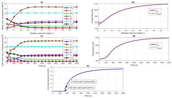
Figure 4.
(a) Steady state profile for molar concentration of species; (b) Steady state profile for gas and catalyst temperatures; (c) Dynamic profile for molar concentration of species at reformer exit; (d) Dynamic profile for gas and catalyst temperatures at reformer exit; (e) Pressure in the line pack.
The dynamic profiles of the exit molar concentration of each species taking part in the reforming reactions are illustrated in Figure 4c. It can be noticed from the profile that the molar concentrations of the species settle to their steady state values in approximately 600 s. The exit molar concentration of and CO increase while that for all the other species decrease with time as they are consumed in the reforming reactions. , which is an inert component does not take part in any of the reactions and thus exhibits a constant profile. As the exothermic reactions dominates the endothermic reactions, the gas temperature and catalyst temperature profiles at the reformer exit are found to be increasing with time as seen in Figure 4d and settle at a value of approximately 1090 K.
As already discussed, before the plant start-up, some amount of hydrogen is assumed to be present between the pipeline connecting NRV to the control valve 2 to maintain a pressure of 1 atm. The NRV after the membrane separation unit (see Figure 1) restricts the flow of hydrogen further from the reformer exit through the membrane to the control valve 2 inlet until the upstream pressure (membrane permeate side) exceeds the downstream pressure (line pack pressure maintained at 1 atm initially). As can be seen from Figure 4e, the NRV remains closed till a time period of 341 s, after which it opens to allow flow of hydrogen to build up the line pack pressure beyond 1 atm. As can be seen from Figure 4e, the plant is designed in such a manner that as the line pack pressure increases and becomes 1.1 times greater than the downstream pressure (1 atm), the control valve 2 is opened to 50% (at 362 s as seen from Figure 4e). The initially closed control valve 2 allows the molar concentration of in the line pack to build up (in turn causing a build up in the line pack pressure) as shown in Figure 5a. In response to the sudden opening of the control valve 2, the profiles for line pack pressure and molar concentration of in the line pack starts increasing as can be seen from Figure 4e and Figure 5a respectively.
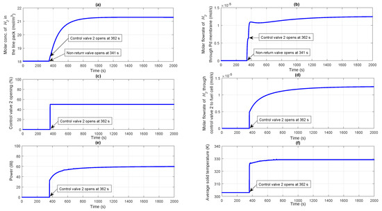
Figure 5.
(a) Molar concentration of in the line pack; (b) Molar flow rate of through Pd membrane; (c) Percentage opening of the control valve 2; (d) Molar flow rate of through control valve 2 to fuel cell; (e) Power generated by a single fuel cell; (f) Average solid temperature of fuel cell.
According to the Sievert’s law given by Equation (13), the molar flow rate of hydrogen permeating through the palladium membrane represented by increases as soon as the NRV opens at 341 s (see Figure 5b). At 362 s, when control valve 2 opens, a small disturbance is expected in the molar flow rate of hydrogen as can be understood from Sievert’s law given by Equation (13). In response to opening of the control valve to 50% at 362 s (see Figure 5c), pressurized from the line pack starts flowing through the control valve 2 to the fuel cell anode, the molar flow rate of which can be seen from Figure 5d. As the molar flow rate of to the fuel cell anode increases in response to opening of the control valve 2, the electrochemical reactions commence, which in turn increases the power generated by the fuel cell as shown in Figure 5e. From the start up simulation, it can be observed that the dynamics of reformer-membrane-fuel cell is sluggish. This is because of lack of availability of for 362 s, when the control valve 2 opens to 50% once the line pack pressure exceeds 1.1 times the downstream fuel cell pressure. However, as can be seen from Figure 5b,d, the flow rate from the membrane to the line pack limits the flow rate of to the fuel cell. Thus, the fuel cell dynamics are slower due to the limitation of the hydrogen produced by the reformer. The dynamics associated with shut-down of the integrated system has not been studied in the current work. The mathematical modeling of the ancillary components like heaters, mixers etc. are not taken into account for this particular study for simplification. Due to the dominating exothermic reactions occurring in the auto thermal reformer, there is always a possibility for cogeneration which can enhance the overall efficiency of the plant. The heat extracted by the coolant from the PEM fuel cell can also be used for heat transfer to the fuel. This will be a subject matter for our future work. The average solid temperature of the fuel cell increases and settles to a value of approximately 330 K as can be seen from Figure 5f, which is based on a constant coolant circulation flow rate of 0.055 mol s−1.
Relative Gain Array (RGA) Analysis
The controlled variables chosen in this particular study are the molar concentration of in the line pack (or pressure in the line pack assuming ideal gas law) (), power demanded by the output electrical load () and average solid temperature of the fuel cell (). For achieving satisfactory operation of the integrated reformer membrane fuel cell assembly, the available manipulated variables selected are the molar flow rate of to the reformer inlet through control valve 1 (), molar flow rate of to the fuel cell anode through control valve 2 () and molar flow rate of coolant to the fuel cell through control valve 3 (). For designing appropriate single input single output (SISO) controllers to form a multi-loop control strategy, suitable input-output pairings need to be decided for which the RGA analysis is carried out. By performing step changes in the manipulated variables and observing the changes in output variables of the integrated system, steady state model of the system in deviation form is obtained as,
Given the steady state gain matrix K of the system, the steady-state RGA matrix for the selected inputs and outputs can be obtained by Equation (40).
It can be noticed that the RGA for diagonal pairings (), () and () are 1.0638, 0.7047 and 0.6730 respectively which is closer to 1 indicating stronger interaction. This pairing seems appropriate from a process point of view because the molar flow rate of to the reformer inlet through control valve 1 () has a direct effect on the amount of produced at the reformer output which in-turn has an effect on the molar concentration of in the line pack (or pressure in the line pack assuming ideal gas law) (). Similarly, the molar flow rate of to fuel cell anode through control valve 2 () has a direct effect on the power demanded by the output electrical load (). Also, the molar flow rate of coolant circulated through the fuel cell () has a direct effect on the average solid temperature of fuel cell (). As can be seen from the steady-state RGA matrix, the RGA for off-diagonal pairings are negative and/or are far way from 1 indicating lesser interaction. A process flow diagram with selected input-output pairings and with appropriate control loops is shown in Figure 6.
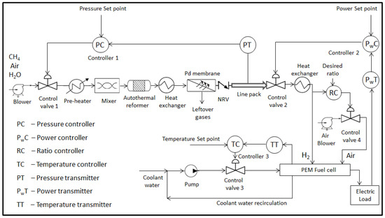
Figure 6.
Process flow diagram with control loops for the integrated system.
3.2. Case Study 2: Integrated System Delivering Target Power Demand
For validating the capability of employing the integrated system for a realistic application, an electrical load of about 27 kW is considered, which corresponds to a light motor vehicle [26], powered by an integrated reformer membrane fuel cell system. Taking into account the transmission and DC/AC converter losses, the maximum power requested is assumed to be 30 kW. In this particular case study, the PEM fuel cell modeled can generate a maximum current density of 1.5319 A cm−2 at a cell voltage of 0.53 V based on the model parameters used. As the electrode area per cell is assumed to be 100 cm, a single fuel cell can generate a maximum power of approximately 0.08 kW. In order for the fuel cell to generate a power of 30 kW, a fuel cell stack consisting around 375 such individual cells connected in series is necessary. Modeling a fuel cell stack containing these many cells is beyond the scope of this paper. For the purpose of simulating the fuel cell stack, it is assumed here that each cell in the stack behaves identically. Thus, the overall stack voltage will be given by the sum of 375 individual cell voltages given by Equation (31). The average molar flow rate of hydrogen for the fuel cell system is mol s−1 or mol h−1. This corresponds to a methane flow rate of 15.12 mol h−1. Assuming that methane is stored at 200 atm pressure and a temperature of 298 K and using ideal gas law, the corresponding volume of methane is 1.8 litres. The output electrical load power demand is assumed to exhibit slower dynamics for the first 65 s and extremely faster dynamics during rest of the time. In this case study, controller 1 tries to regulate the molar concentration of in the line pack to 21.315 mol m−3 irrespective of variation in the power requested by the fuel cell. This is achieved by manipulating the control valve 1 position thereby varying the molar flow rate of fuel to the reformer inlet. In other words, controller 1 controls the hydrogen pressure in the line pack by manipulating the methane flow rate to the reformer inlet. Line pack pressure is calculated from the molar concentration of hydrogen present in the line pack using the ideal gas law as given by Equation (37). Inlet pressure at the anode and cathode sides are fixed at 1 atm. Line pack pressure control ensures presence of sufficient hydrogen always to prevent hydrogen starvation, which can permanently damage the fuel cell stack. The molar concentration of in the line pack is chosen as the controlled variable keeping the molar flow rate of fuel from the fuel storage to the reformer inlet through the control valve 1 as the manipulated variable. In addition to this, controller 2 is designed to take necessary action to supply requisite amount of to fuel cell anode in order to achieve the desired target power. Output power demanded by the fuel cell stack is identified as the controlled variable while the molar flow rate of through the control valve 2 to the fuel cell anode is selected as the manipulated variable. Third loop involves controller 3 and is designed to maintain a fixed average solid temperature of fuel cell by manipulating the molar flow rate of coolant circulated. As obvious, average solid temperature is selected as the controlled variable while molar flow rate of coolant is selected as the corresponding manipulated variable. Finally, fourth loop involves a ratio controller that regulates the ratio of air to hydrogen to be fed to the cathode and anode inlets of the fuel cell respectively. The tuning parameters for the four controllers are listed in Table 2.
Table 2.
Design parameters for various control loops.
Based on the power demanded by the fuel cell load, the controller 2 manipulates the control valve 2 position as shown in Figure 7a. Opening of the control valve 2 lets an appropriate amount of to flow to the fuel cell anode, the molar flow rate of which can be seen from Figure 7b. Due to the feedback mechanism, controller 1 takes necessary action to manipulate the percentage opening of control valve 1 as shown in Figure 7c.
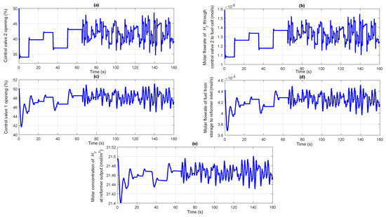
Figure 7.
(a) Percentage opening of the control valve 2; (b) Molar flow rate of through control valve 2 to fuel cell; (c) Percentage opening of the control valve 1; (d) Molar flow rate of fuel from storage to reformer inlet; (e) Molar concentration of at reformer output.
Proportionately, the molar flow rate of stored fuel coming as input to the reformer starts varying as illustrated in Figure 7d. In response to this, the molar concentration of exiting from the reformer also starts varying as given in Figure 7e. According to Sievert’s law given by Equation (13), in response to variation in the molar concentration of coming from the reformer, the molar flow rate of flowing through the Pd membrane starts varying as is obvious from Figure 8a. The controller 1 takes necessary action to maintain a constant molar concentration in the line pack between NRV and control valve 2 as shown in Figure 8b. As can be seen from the figure, the dashed line indicates the desired target molar concentration to be maintained while the solid line indicates the actual concentration in the line pack. As already discussed, the variation in the molar flow rate of to the fuel cell anode changes the power generated by the fuel cell which can be seen from Figure 8c. The dashed line shows the desired target power demanded by the electrical load while the solid line indicates the actual power supplied by the PEMFC. The profile showing the variation in the line pack pressure is given in Figure 8d. The controller 3 takes care of maintaining the average solid temperature of the fuel cell at a desirable value irrespective of variations in the power demanded by the fuel cell electric load. The manipulation of coolant flow rate by varying the control valve 3 position by the controller 3 can be observed from Figure 8e. The corresponding profile for the average solid temperature of the PEMFC is shown in Figure 8f. It is observed that the designed controllers with appropriately chosen controller parameters were able to control the molar concentration in the line pack, fuel cell power demand and the average solid temperature of fuel cell with relatively short settling times and with negligible offset. Both slow and fast varying load scenarios have been simulated in the present case study for the closed loop system for power control and observed that the designed controller could tracks the set point with a settling time of the order of 0.4 s.
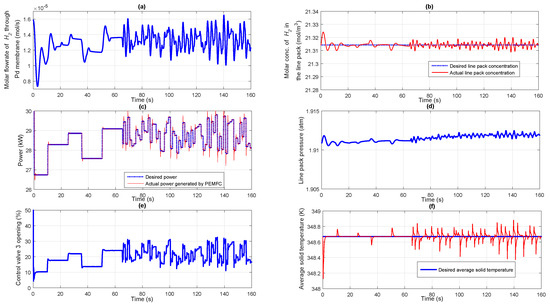
Figure 8.
(a) Molar flow rate of through Pd membrane; (b) Performance of controller 1 maintaining a fixed molar concentration of in the line pack; (c) Performance of controller 2 tracking the target power profile; (d) Pressure in the line pack; (e) Percentage opening of the control valve 3; (f) Performance of controller 3 maintaining a fixed average solid temperature of fuel cell.
3.3. Case Study 3: Disturbance in both the Reformer Inlet Feed Concentration and Coolant Temperature
The ability of the designed controller to reject the unknown disturbances occurring in the integrated reformer membrane fuel cell system is analyzed in this case study. In the previous case study, it was assumed that the inlet concentration and coolant temperature are fixed and are not affected by any external disturbances. In this particular case study, disturbance in the form of step change is introduced in both the inlet concentration as well as coolant temperature as shown in Figure 9a,b respectively. The control structure discussed here is also similar to the one discussed in the previous case study. Controller 1 tries to maintain a fixed molar concentration of in the line pack by manipulating the flow rate of fuel entering the reformer while controller 2 make sure that the power demanded by the electrical load is delivered by the fuel cell at the appropriate time. Controller 3 maintains a fixed average solid temperature in the fuel cell irrespective of changes in the output power demand as well as variations in the coolant flow rate and temperature. Based on the power demanded by the fuel cell electrical load, controller 2 manipulates the control valve 2 as seen from Figure 9c. Based on the opening of control valve 2, the requisite amount of flows to the fuel cell anode, the molar flow rate of which is shown in Figure 9d. Once the concentration in the line pack gets disturbed, controller 1 takes necessary action to manipulate the opening of control valve 1 so as to maintain the line pack concentration at a constant value. The change in control valve 1 opening based on the command from the controller 1 can be seen from Figure 9e. Based on the control valve 1 opening, appropriate amount of stored fuel is supplied as input to the auto thermal reformer, the molar flow rate of which can be seen in Figure 9f. Because of the presence of impurities in concentration at the inlet, controller 1 takes additional action so as to compensate for the unknown disturbance happening at the input side of the plant. As the fuel inlet to the reformer varies, the molar concentration of at the reformer output also starts varying as shown in Figure 10a. Accordingly, the molar flow rate of passing through the Pd membrane also starts varying as given in Figure 10b. The profile showing the desired and the actual molar concentration of in the line pack is shown in Figure 10c. It can be seen from Figure 10d that the power demanded by the electrical load and actual power delivered by the fuel cell. Because of the presence of disturbance in the coolant flow rate as well as changes in the power demanded, the average solid temperature starts varying from the required set point value. A significant deviation in the fuel cell power compared to the desired power at the initial time period (first 5 s) can be observed from Figure 10d. This is due to the disturbance in the coolant inlet temperature from its nominal value of 340 K to 345 K, as observed from Figure 9b. This in turn resulted in loss of power, due to which, controller 3 increases the coolant flow rate which restores the temperature of the fuel cell and consequently the power (see Figure 10d,e). Based on the command from the controller 3, the average solid temperature sticks to the pre-defined set value as can be seen from Figure 10f. It is observed that the designed controllers with appropriately chosen controller parameters were able to control the parameters and track the set point even in the presence of unexpected disturbances happening in the plant. Due to the presence of disturbances, the deviations of molar concentration of hydrogen in the line pack as well as the average solid temperature from the set point is more compared to the scenario when disturbances were absent.
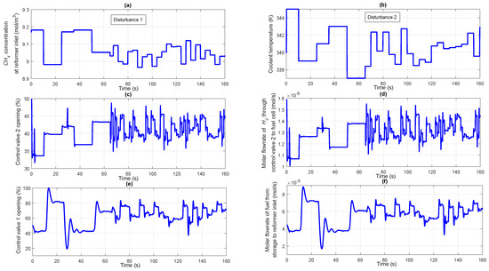
Figure 9.
(a) Disturbance in the concentration of at reformer inlet; (b) Disturbance in the coolant temperature; (c) Percentage opening of the control valve 2; (d) Molar flow rate of through control valve 2 to fuel cell; (e) Percentage opening of the control valve 1; (f) Molar flow rate of fuel from storage to reformer inlet.
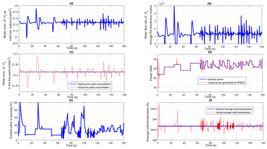
Figure 10.
(a) Molar concentration of at reformer output; (b) Molar flow rate of through Pd membrane; (c) Performance of controller 1 maintaining a fixed molar concentration of in the line pack; (d) Performance of controller 2 tracking the target power profile; (e) Percentage opening of the control valve 3; (f) Performance of controller 3 maintaining a fixed average solid temperature of fuel cell.
4. Conclusions
A system level mathematical model of an integrated reformer membrane fuel cell system has been developed in order to assess the feasibility of the integrated system for stationary and portable power applications. Such an integrated system promotes safety and leverages existing natural gas infrastructure. The dynamic analysis of the open loop system revealed significant difference in the dynamics related to the upstream reformer as compared with the fuel cell. This behavior points the need for an auxiliary power system during startup of the integrated system which is outside the scope of this work. A multi loop control strategy is implemented on to the integrated system wherein power demanded by the fuel cell load, molar concentration of in the line pack and average solid temperature of the fuel cell are chosen as the controlled variables for the two control loops. Relevant controllers are designed appropriately to control the system which included set point tracking and disturbance rejection studies. The simulation results show faster settling times with negligible offset proving the effectiveness of the designed controller.
Author Contributions
All of the authors contributed to publishing this article. The collection of materials and summarization of this article was done by P.P.S. and the conceptual ideas, methodology and guidance for the research were provided by R.D.G. and S.B. All the coding and programming works was done by P.P.S.
Funding
This research was funded by the Dept. of Science & Technology, Govt. of India, Grant 13DST057.
Conflicts of Interest
The authors declare no conflict of interest.
Nomenclature
| ratio of water molecules per proton (molecules proton) | |
| heat of reaction (kJ mol) | |
| packing bed porosity | |
| effectiveness factor of reaction j | |
| over potential (V) | |
| effective thermal conductivity (W(mK)) | |
| water viscosity (g cms) | |
| density of the catalyst bed (kg m) | |
| density of the catalyst pellet (kg m) | |
| density of the fluid (kg m) | |
| density of the solid (kg m) | |
| density of dry membrane of fuel cell (g cm) | |
| ionic conductivity of the fuel cell membrane (Ohm cm) | |
| Pd membrane poisoning caused by the adsorption of | |
| A | heat exchange area per unit length (cm) |
| area of the fuel flow pipe to the reformer inlet (m) | |
| activity of water in stream k | |
| external catalyst surface area per unit volume of catalyst bed (mm) | |
| Pd membrane surface area (m) | |
| molar concentration of species i in the gas phase (mol m) | |
| molar heat capacity (J(g mol K)) | |
| concentration of water in the membrane of fuel cell (mol cm) | |
| molar concentration of in the line pack (mol m) | |
| molar concentration of species i in the solid phase (mol m) | |
| specific heat of the catalyst bed (J (kg K)) | |
| specific heat of the fluid (J (kg K)) | |
| control valve 1 flow coefficient | |
| control valve 2 flow coefficient | |
| concentration of water at k interface of the membrane of fuel cell (mol cm) | |
| D | diffusion coefficient of water in membrane of fuel cell (cm s ) |
| d | fuel cell channel height (cm) |
| axial dispersion coefficient (m s ) | |
| e | membrane area per unit length (cm) |
| activation energy for permeability (J mol) | |
| F | Faraday’s constant (C mol) |
| f | cross-section of solid in fuel cell (cm) |
| opening of control valve 1 (%) | |
| opening of control valve 2 (%) | |
| piping geometry factor | |
| h | fuel cell channel width (cm) |
| gas to solid heat transfer coefficient (W ms) | |
| I | current density (A cm) |
| exchange current density (A cm) | |
| k | heat conduction coefficient (W (cmK)) |
| condensation rate constant (s) | |
| parameter corresponding to the viscous loss term (Pa s m) | |
| parameter corresponding to the kinetic loss term (Pa s m) | |
| gas to solid mass transfer coefficient of component i (m s) | |
| Pd membrane thickness (m) | |
| M | molar flow rate (mol s) |
| equivalent weight of dry membrane of fuel cell (g mol) | |
| n | pressure exponent |
| number of electrons taking part in charge reactions | |
| molar flux of species i (mol s cm) | |
| P | pressure (atm) |
| vapor pressure of water in channel | |
| permeability of Pd membrane (mol (msPa) | |
| permeability pre-exponential factor (mol (msPa) | |
| methane fuel storage pressure (atm) | |
| R | gas constant (J (mol K)) |
| rate of consumption or formation of species i (mol (kgs)) | |
| rate of reaction j (mol (kgs)) | |
| t | time (s) |
| reformer gas temperature (K) | |
| fuel cell membrane thickness (cm) | |
| fuel cell solid temperature (K) | |
| gas temperature at the exit of heat exchanger 1 (K) | |
| ambient temperature (K) | |
| methane fuel storage temperature (K) | |
| U | convective heat transfer coefficient (W cm K) |
| u | superficial gas flow velocity (m s) |
| V | volume of the line pack (m) |
| cell voltage (V) | |
| open circuit voltage (V) | |
| W | molecular weight (kg mol) |
| X | ratio of pressure drop to the absolute inlet pressure |
| x | direction along the fuel cell channel length (cm) |
| Y | expansion factor |
| Z | compressibility factor |
| z | axial dimension (m) |
Suffixes
| a | anode |
| c | cathode |
| g | gas |
| m | line pack |
| s | solid |
| sat | saturation |
| w | water |
Appendix A. Data for the Base Case
| Parameter | Values |
| (mol m) | 9.1705 |
| (mol m) | 4.1273 |
| (mol m) | 0.0001 |
| (mol m) | 9.1705 |
| (mol m) | 0.0001 |
| (mol m) | 0.0001 |
| (mol m) | 15.5287 |
| (K) | 815 |
| (K) | 815 |
| (mol m) | 0.001 |
| (mol s) | |
| (mol s) | |
| (mol s) | 0 |
| (mol s) | 0 |
| (mol s) | |
| (mol s) | |
| (K) | 353 |
| (K) | 353 |
| (K) | 340 |
| (K) | 342 |
Appendix B. Parameter Values Used for Simulation
| Parameter | Values |
| 0.4 | |
| z (m) | 0.2 |
| (m s) | |
| (m) | 1200 |
| (kg m) | 1870 |
| (kg m) | 1122 |
| (J kg K) | 850 |
| (kJ mol) | 206.2 |
| (kJ mol) | 164.9 |
| (kJ mol) | −41.1 |
| (kJ mol) | −802.7 |
| (K) | 0.07 |
| (K) | 0.06 |
| (K) | 0.7 |
| (K) | 0.05 |
| (K) | |
| 0.2 | |
| (m) | 0.0064 |
| (m) | 0.0001 |
| R (J mol K) | 8.314 |
| n | 0.67 |
| (mol m s Pa) | 0.4 |
| (J mol) | 8000 |
| x (cm) | 10 |
| h (cm) | 0.1 |
| d (cm) | 0.1 |
| F (C mol) | 96484.69 |
| (s) | 100 |
| (atm) | 1 |
| (atm) | 1 |
| (W cm K) | 0.025 |
| (cm) | 0.4 |
| (W cm K) | 0.025 |
| (cm) | 0.4 |
| (J g mol K) | 75.38 |
| (mol s) | |
| (g cm) | 2 |
| (J g mol K) | 1 |
| (W cm K) | 0.005 |
| e (cm) | 0.1 |
| (W cm K) | 0.025 |
| (K) | 350 |
| (V) | 1.1 |
| (cm) | 0.01275 |
| 2 | |
| (A cm) | 0.01 |
| 0.667 | |
| 0.67 | |
| Y | 1 |
| (kg mol) | 0.016 |
| Z | 1 |
| (atm) | 2 |
| V (m) | 0.00025 |
| 0.002 | |
| (kg mol) | 0.002 |
References
- Qi, A.; Peppley, B.; Karan, K. Integrated fuel processors for fuel cell application: A review. Fuel Process. Technol. 2007, 88, 3–22. [Google Scholar] [CrossRef]
- Halabi, M.; de Croon, M.; van der Schaaf, J.; Cobden, P.; Schouten, J. Modeling and analysis of autothermal reforming of methane to hydrogen in a fixed bed reformer. Chem. Eng. J. 2008, 137, 568–578. [Google Scholar] [CrossRef]
- Iwuchukwu, I.J.; Sheth, A. Mathematical modeling of high temperature and high-pressure dense membrane separation of hydrogen from gasification. Chem. Eng. Process. Process. Intensif. 2008, 47, 1292–1304. [Google Scholar] [CrossRef]
- Okazaki, J.; Ikeda, T.; Tanaka, D.A.P.; Sato, K.; Suzuki, T.M.; Mizukami, F. An investigation of thermal stability of thin palladium–silver alloy membranes for high temperature hydrogen separation. J. Membr. Sci. 2011, 366, 212–219. [Google Scholar] [CrossRef]
- Authayanun, S.; Mamlouk, M.; Scott, K.; Arpornwichanop, A. Comparison of high-temperature and low-temperature polymer electrolyte membrane fuel cell systems with glycerol reforming process for stationary applications. Appl. Energy 2013, 109, 192–201. [Google Scholar] [CrossRef]
- Basualdo, M.; Feroldi, D.; Outbib, R. PEM Fuel Cells with Bio-Ethanol Processor Systems: A Multidisciplinary Study of Modelling, Simulation, Fault Diagnosis and Advanced Control. In Green Energy and Technology; Springer: London, UK, 2011. [Google Scholar]
- Lorenzo, G.D.; Corigliano, O.; Faro, M.L.; Frontera, P.; Antonucci, P.; Zignani, S.; Trocino, S.; Mirandola, F.; Aricò, A.; Fragiacomo, P. Thermoelectric characterization of an intermediate temperature solid oxide fuel cell system directly fed by dry biogas. Energy Convers. Manag. 2016, 127, 90–102. [Google Scholar] [CrossRef]
- Kupecki, J.; Motylinski, K.; Milewski, J. Dynamic analysis of direct internal reforming in a sofc stack with electrolyte-supported cells using a quasi-1d model. Appl. Energy 2018, 227, 198–205. [Google Scholar] [CrossRef]
- Lorenzo, G.D.; Milewski, J.; Fragiacomo, P. Theoretical and experimental investigation of syngas-fueled molten carbonate fuel cell for assessment of its performance. Int. J. Hydrogen Energy 2017, 42, 28816–28828. [Google Scholar] [CrossRef]
- El-Sharkh, M.; Rahman, A.; Alam, M.; Byrne, P.; Sakla, A.; Thomas, T. A dynamic model for a stand-alone pem fuel cell power plant for residential applications. J. Power Sources 2004, 138, 199–204. [Google Scholar] [CrossRef]
- Ipsakis, D.; Voutetakis, S.; Seferlis, P.; Papadopoulou, S.; Stoukides, M. Modeling and analysis of an integrated power system based on methanol autothermal reforming. In Proceedings of the 17th Mediterranean Conference on Control and Automation, Thessaloniki, Greece, 24–26 June 2009; pp. 1421–1426. [Google Scholar]
- Stamps, A.T.; Gatzke, E.P. Dynamic modeling of a methanol reformer- pemfc stack system for analysis and design. J. Power Sources 2006, 161, 356–370. [Google Scholar] [CrossRef]
- Patcharavorachot, Y.; Wasuleewan, M.; Assabumrungrat, S.; Arpornwichanop, A. Analysis of hydrogen production from methane autothermal reformer with a dual catalyst-bed configuration. Theor. Found. Chem. Eng. 2012, 46, 658–665. [Google Scholar] [CrossRef]
- Ding, O.; Chan, S. Autothermal reforming of methane gas-modelling and experimental validation. Int. J. Hydrogen Energy 2008, 33, 633–643. [Google Scholar] [CrossRef]
- Vadlamudi, V.K.; Palanki, S. Modeling and analysis of miniaturized methanol reformer for fuel cell powered mobile applications. Int. J. Hydrogen Energy 2011, 36, 3364–3370. [Google Scholar] [CrossRef]
- Pinacci, P.; Drago, F. Influence of the support on permeation of palladium composite membranes in presence of sweep gas. Catal. Today 2012, 193, 186–193. [Google Scholar] [CrossRef]
- Doong, S.; Yang, R. Hydrogen purification by the multibed pressure swing adsorption process. React. Polym. Ion Exch. Sorbents 1987, 6, 7–13. [Google Scholar] [CrossRef]
- Canevese, S.; Marco, A.D.; Murrai, D.; Prandoni, V. Modelling and control of a psa reactor for hydrogen purification. IFAC Proceed. Vol. 2007, 40, 99–104. [Google Scholar] [CrossRef]
- Bhargav, A. Model Development and Validation of Palladium-Based Membranes for Hydrogen Separation in Pem Fuel Cell Systems. Ph.D. Thesis, University of Maryland, College Park, MD, USA, 2010. [Google Scholar]
- Golbert, J.; Lewin, D.R. Model-based control of fuel cells: (1) Regulatory control. J. Power Sources 2004, 135, 135–151. [Google Scholar] [CrossRef]
- Pukrushpan, J.T.; Stefanopoulou, A.G.; Peng, H. Modeling and control for pem fuel cell stack system. In Proceedings of the 2002 American Control Conference (IEEE Cat. No.CH37301), Anchorage, AK, USA, 8–10 May 2002; Volume 4, pp. 3117–3122. [Google Scholar]
- Nguyen, T.; White, R. A water and heat management model for proton-exchange-membrane fuel cells. J. Electrochem. Soc. 1993, 140, 2178–2186. [Google Scholar] [CrossRef]
- Methekar, R.; Prasad, V.; Gudi, R. Dynamic analysis and linear control strategies for proton exchange membrane fuel cell using a distributed parameter model. J. Power Sources 2007, 165, 152–170. [Google Scholar] [CrossRef]
- Perry, R.H.; Green, D.W.; Maloney, J.O. Perry’s Chemical Engineers Handbook, 7th ed.; The McGraw-Hill Companies Inc.: New York, NY, USA, 1999. [Google Scholar]
- Chatrattanawet, N.; Skogestad, S.; Arpornwichanop, A. Control structure design and dynamic modeling for a solid oxide fuel cell with direct internal reforming of methane. Chem. Eng. Res. Des. 2015, 98, 202–211. [Google Scholar] [CrossRef]
- Sarkar, A.; Banerjee, R. Net energy analysis of hydrogen storage options. Int. J. Hydrog Energy 2005, 30, 867–877. [Google Scholar] [CrossRef]
© 2018 by the authors. Licensee MDPI, Basel, Switzerland. This article is an open access article distributed under the terms and conditions of the Creative Commons Attribution (CC BY) license (http://creativecommons.org/licenses/by/4.0/).