Enhancing Point Cloud Registration Precision of Conical Shells Through Edge Detection Using PCA and Wavelet Transform

Abstract

Reliability assessment of conical shells in the chemical industry commonly relies on point cloud registration. Thus, accurate edge detection from 3D laser scan data is crucial for high-precision registration. However, existing edge detection methods often misclassify or omit gradual edge points on conical shell structures, significantly compromising registration accuracy and subsequent integrity assessment. This paper proposes an edge point detection method integrating Principal Component Analysis (PCA) and wavelet transform. First, characteristic curves are constructed by computing the ratio of PCA eigenvalues at all points to generate preliminary candidates for gradual edge points. Subsequently, distance vectors are calculated between the centroid of each characteristic curve and its sampled points. These vectors are then encoded via multi-level wavelet transform to produce mapping vectors that capture curvature variations. Finally, gradual edge points are discriminated effectively using these mapping vectors. Experimental results demonstrate that the proposed method achieves superior edge detection performance on complex conical shell surfaces and significantly enhances the accuracy of point cloud registration.

1. Introduction

Conical shells are essential components in chemical and petrochemical industries, serving as critical infrastructure for the storage of fuels, solvents, and other industrial liquids [1]. During manufacturing and long-term operation, these pressure vessels are frequently subjected to corrosion, local deformation, and weld distortion, which can lead to structural defects and threaten process safety [2]. Identifying and evaluating these defects is crucial for maintaining operational reliability and ensuring environmental protection [3]. In recent years, with the maturation of 3D laser scanning technology, high-resolution point cloud data have provided a reliable means for non-contact measurement [4], enabling refined geometric inspection of conical shells. Within this technical framework, edges—representing regions where geometric attributes change abruptly—play an important role in describing structural contours and identifying critical areas [5]. High-accuracy point cloud registration is a central step in the precise measurement of conical shells, and effective edge detection directly contributes to improved registration quality [6]. Therefore, accurately extracting edge features from point clouds is not only key to registration accuracy but also lays a solid foundation for subsequent structural integrity analysis and safety monitoring.

In practice, however, edge detection for complex curved surfaces of conical shell faces significant challenges [7]. The geometric regions of conical shells are diverse, including planar regions, intersection regions, and open boundaries (among them, intersection regions consist of sharp edge points and edge points with gradual transition features). Many intersection regions contain gradual edge points, where curvature changes smoothly rather than sharply. Conventional edge detection methods often fail to accurately identify such gradual edge points, resulting in missed detections or unstable registration outcomes. Therefore, a central challenge in this field remains the accurate detection of gradual edge points (edge points with gradual transition features) to enhance point cloud registration accuracy. Notably, most existing edge detection methods are effective for sharp edge points. However, they often fail to reliably identify the multiple edge point types in conical shells, leading to both false positives and missed detections, particularly for gradual edge points. To overcome these limitations, this paper proposes a novel edge detection algorithm utilizing PCA and wavelet transform. The main contributions of this work are summarized as follows:

(1)

A characteristic curve model based on PCA eigenvalue ratios, which is constructed across expanding neighborhood radius to capture geometric transitions and classify geometric regions of conical shells.

(2)

Using distance vectors to represent characteristic curves, providing a pathway for distinguishing between planar points and gradual edge points.

(3)

Wavelet-based mapping vectors encoding scheme that ensures rotation translation invariance and distance consistency, enhancing the discrimination of gradual edge points.

(4)

Comprehensive experimental evaluation, including gradual edge detection, multi-type edge detection, and point cloud registration studies, demonstrating the method’s high precision.

The proposed method not only reliably identifies diverse edge point types but also demonstrates superior performance in detecting gradual edge points. By accurately identifying edge points, the proposed approach improves the precision of point cloud registration.

The rest of this paper is organized as follows. Section 2 reviews existing methodologies for point cloud edge detection and discusses their limitations. Section 3 details the proposed method, including the construction of characteristic curves, distance vectors, and wavelet-based mapping vectors. Section 4 presents experimental results and analysis, covering gradual edge detection, multi-type edge detection, and point cloud registration. Section 5 concludes the paper. Section 6 investigates the limitations of our method and outlines potential directions for future work.

2. Related Works

Recent research has categorized point cloud edge detection methods into three main types: surface transformation-based, graph-based, and local neighborhood geometry-based methods.

Surface transformation-based methods can be broadly categorized into two approaches: those that extract features by fitting surfaces to local regions, and those that do so by meshing the local regions. Daniels et al. employed an iterative projection technique to map the point cloud onto the intersection lines of adjacent surfaces, enabling the identification of sharp edge points [8]. A limitation of this method is its tendency to generate jagged edge lines at the junctions of complex surfaces. To improve the geometric consistency of feature lines, Yutaka et al. proposed a multilevel implicit surface fitting method [9]. While this approach enhanced fitting accuracy, it was accompanied by a significant increase in computational complexity. Other studies have explored mesh-based conversion of 3D features to reduce computational demands. For instance, Demarsin et al. achieved a balance between computational efficiency and the completeness of detected edge points by fitting a grid structure [10]. A common drawback of these methods, however, is their overemphasis on detection of sharp edge points, often overlooking the critical information provided by gradual edge points. To address this, the proposed method introduces characteristic curves that capture gradual edge points by analyzing eigenvalues across varying neighborhood radius, thereby enhancing sensitivity to gradual curvature changes.

Graph-based methods regard edge detection as a high-pass filtering strategy in the graph signal processing framework, as edge features are usually considered to correspond to the high-frequency components of the graph signal. Chen et al. designed a high-pass graph filter by minimizing the reconstruction error of the Haar-like graph, thereby obtaining the optimal resampling distribution for point cloud edges [11]. To further improve the quality of point cloud resampling, Qi et al. proposed a resampling loss function that more effectively retains edge features while maintaining sampling uniformity [12]. However, the traditional two-dimensional graph structure is inherently limited in its ability to fully represent three-dimensional point clouds. In this regard, Deng et al. proposed a graph filtering method based on high-dimensional space hypergraphs, which more comprehensively captures structural information within the original point cloud, thereby enhancing the detection of edge features [13]. Although graph signal processing methods are proficient at detecting sharp edge points, their high-frequency sensitivity makes them prone to missing gradual edge points, thereby reducing their robustness in complex scenarios. Our approach mitigates this by employing wavelet-based mapping vectors that encode the curvature variations in gradual edge points, thereby capturing gradual edge features without over-reliance on high-frequency components.

Methods based on local neighborhood geometry primarily utilize changes in the local geometric structure of a point cloud to evaluate each point, considering attributes such as normal, curvature, and surface variation. Xia et al. proposed a geometric center edge detector that identifies edge structures through gradient features [14]. However, such methods are highly dependent on the selection of neighborhood radius, which compromises the robustness of feature detection. To address this limitation, Zhang et al. introduced a Poisson distribution model to enhance feature recognition via adaptive normal estimation [15]. Essentially, however, this approach remains a form of single-feature statistics and does not establish multi-dimensional geometric correlations. Against this background, covariance matrix analysis has emerged as a new direction for feature detection. Dena et al. adopted a K-nearest neighbor covariance eigenvalue decomposition method, which effectively mitigates cross-edge neighborhood interference inherent in traditional gradient-based methods and improves the detection accuracy of sharp edge points [16]. Nevertheless, this method suffers from discontinuous edges with gradual transition features. To overcome this, Pauly et al. constructed a multi-scale geometric feature classification framework [17]. By quantifying the degree of surface variation at different scales, they extended the adaptability of feature detection to a wider range of geometric forms. However, this framework still generates significant false detections when handling gradual edge points. Furthermore, Quentin et al. proposed an improvement to edge detection by replacing the traditional covariance matrix with Voronoi cell covariance, thereby enhancing the ability to detect sharp edge points [18]. Notably, these methods generally rely on a fixed neighborhood analysis strategy and do not establish a dynamic correlation model between feature parameters and neighborhood radius, leading to inaccurate identification of edge point types. In contrast, our method constructs characteristic curves over a range of neighborhood radius and employs distance vectors combined with wavelet transforms, significantly improving the detection of gradual edge points while reducing sensitivity to radius selection.

3. Methods

For the laser-scanned point cloud of conical shells, this paper adopts principal component analysis (PCA) as a preprocessing step before edge detection. PCA can effectively analyze the principal direction and distribution intensity of the local neighborhood in the point cloud [16]. The specific formula is given as follows:

$$\left\{\begin{array}{c}{p}_c={\displaystyle \frac{1}{\left|N\right|}}{\displaystyle \sum _{p_t\in N}{p}_t}\\ C={\displaystyle \frac{1}{\left|N\right|}}{\displaystyle \sum _{p_t\in N}(p_t-p_c)}{(p_t-p_c)}^T\end{array}\right.$$

(1)

As shown in Figure 1, where $P$ denotes any point in a point cloud. The points $p_t$ are within the local neighborhood $N$ of $P$. $p_c$ is the geometric center of the neighborhood point set. The covariance matrix $C$ is decomposed using eigenvalues:

$$C=V\Lambda V^T$$

(2)

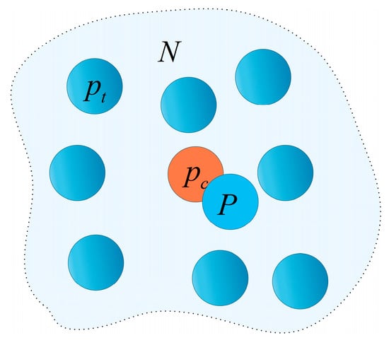
Figure 1. Schematic diagram of point cloud PCA.

Here, $\Lambda =diag({\lambda }_1,{\lambda }_2,{\lambda }_3)$ is a diagonal matrix whose elements satisfy ${\lambda }_1\ge {\lambda }_2\ge {\lambda }_3\ge 0$. These eigenvalues indicate the distribution intensity of the point cloud along the three directions: ${\lambda }_1$ corresponds to the distribution intensity along the principal vector direction (maximum variance), ${\lambda }_2$ corresponds to the distribution intensity along the secondary vector direction, and ${\lambda }_3$ corresponds to the distribution intensity along the normal vector directions (minimum variance). The matrix $V=\left[v_1,v_2,v_3\right]$ is orthogonal, and its column vectors are the eigenvectors associated with the respective eigenvalues, representing the principal vector, secondary vector, and normal vector of the point of $P$.

As shown in Equation (3), this paper establishes a discrimination model for points within each region by constructing the eigenvalue ratio and introducing a neighborhood radius expansion mechanism.

$$\xi ={\displaystyle \frac{{\lambda }_1}{{\lambda }_2}}$$

(3)

Figure 1 categorizes the local neighborhood of a point into three geometric types: planar regions, intersection regions (containing both sharp and gradual edge points), and open boundaries. This classification is achieved by analyzing the spatial distribution through eigenvalue decomposition of the covariance matrix $C$ derived from the neighborhood points. The arrows indicate the expansion direction of the neighborhood, $S_i$ denotes the interior of the point cloud model, and $S_e$ denotes the exterior of the point cloud model.

For the planar region (Figure 2a), since the points in $S_i$ are uniformly distributed, the distribution intensities of the point cloud in all directions calculated by PCA are almost equal. As the neighborhood radius $r$ increases, the number of points distributed in each direction increases with the square of $r$. Therefore, the value of $\xi$ does not change significantly with the increase of $r$ but fluctuates around the base value of 1. For the intersection region (Figure 2b), since the neighborhood points are distributed on two planes, the direction of the planar intersection line contains the largest number of points, so this direction is the principal direction of the point cloud. As $r$ increases, the growth rate of the number of points distributed in this direction is higher than that in the secondary direction. Consequently, the $\xi$ initially increases with $r$. It reaches a maximum value before being constrained by the overall geometry, after which it begins to decrease. This behavior results in a distinct unimodal characteristic curve for $\xi$. For the open boundary (Figure 2c), points are only distributed on the inner side of the model. The boundary direction contains the largest number of points, so this direction is the principal direction of the point cloud. As $r$ increases, the growth rate of the number of points distributed in this direction is higher than that in the secondary direction, therefore showing an increasing trend with the increase of $r$.

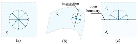
Figure 2. The local neighborhood of a point in the point cloud can be categorized into three geometric types. (a) Plane, (b) intersection, (c) open boundary.

3.1. Edge-Point Classification Model

After the analysis above. The eigenvalue ratio $\xi$, derived from PCA of the point cloud, manifests a strong correlation with the geometric type of the local neighborhood. To illustrate this correlation, we use a second-order conical shell as a case study (Figure 3). On the MATLAB 2024a platform, we demonstrate how $\xi$ varies with the neighborhood radius for the three distinct neighborhood types. As shown in Figure 3, the geometric regions of the second-order ring forging point cloud are visualized and classified according to the three neighborhood types described above. Specifically, blue represents planar regions, red corresponds to open boundaries, and green denotes intersection regions. As illustrated in Figure 4, the blue curve depicts the variation in the eigenvalue ratio for planar points with increasing neighborhood radius, showing stable fluctuations around the baseline value of 1. The red curve represents the variation of $\xi$ for open-boundary points, exhibiting an increasing trend with $r$. The green curve corresponds to intersection edge points, where $\xi$ demonstrates a pronounced unimodal characteristic. Therefore, by performing pattern recognition on the characteristic curve, we can determine the geometric region in which the point is located (Definition: the curve formed by the PCA eigenvalue ratio of a point, as it varies with the increasing neighborhood radius, is referred to as that point’s characteristic curve.). It is noteworthy that, when the neighborhood radius $r<0.6$, the values of the three types of regions exhibit disordered distribution. This explains the difficulty faced by local neighborhood geometry-based methods in finding an appropriate neighborhood, which consequently leads to the misdetection of edge points.

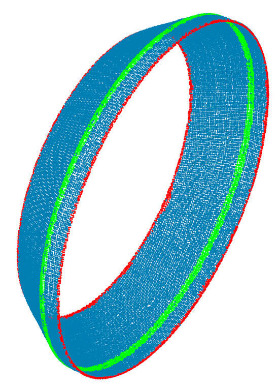
Figure 3. Geometric regions of the second-order conical shell point cloud are visualized and classified.

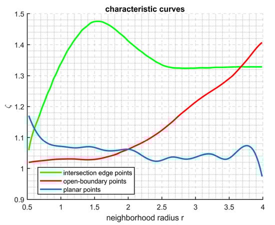
Figure 4. In the three geometric regions, the smoothed characteristic curves show different trends.

To ensure the characteristic curves reflect geometric trends, the radius $r$ varies from $r_{\min }=\overline{d}$ to $r_{\max }=5\overline{d}$ (where $\overline{d}$ denotes the average point spacing in the point cloud). To ensure sufficient fidelity in sampling the characteristic curves and avoid information distortion, the radius sampling interval is set to $\mathrm{\Delta }r=0.1\overline{d}$. This interval is significantly smaller than the Nyquist limit ($0.5\overline{d}$) determined by the point cloud sampling density, thus satisfying the requirements of the Shannon sampling theorem. Consequently, it can effectively capture the variation in the characteristic curves with respect to the radius. As shown in Figure 5a,b, a linear mapping is employed to discretize the continuous radius variable $r$ into a time variable $t\in N^{*}$. The radius increment $\mathrm{\Delta }r$ and the sampling interval $\mathrm{\Delta }t$ satisfy a strict correspondence. By setting the initial sampling interval $\mathrm{\Delta }t$ as a fixed parameter, a sequence ${\left\{\xi \left(t_i\right)\right\}}_{i=1}^N$ is obtained, which represents the discrete characteristic curve.

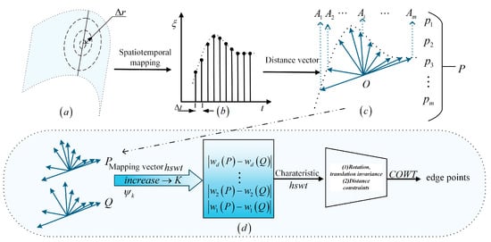
Figure 5. Schematic diagram of point cloud edge extraction strategy. (a) Illustrating radius expansion; (b) Demonstrating space-time mapping; (c) Defining the characteristic curve; (d) Showing the gradual edge points detection strategy.

Pattern recognition of the sequence ${\left\{\xi \left(t_i\right)\right\}}_{i=1}^N$ can determine the geometric region of a point. In real data, the curve is often not ideal. The overall increasing trend may contain local decreases. These fluctuations can cause misjudgment. To address this, we propose a structural analysis method. It uses the ratio of global to segmented variance. This statistic improves the recognition of the overall trend of characteristic curve. Specifically, let the sampling sequence be ${\left\{\xi \left(t_i\right)\right\}}_{i=1}^N$. Its global mean and variance are defined as follows:

$$\left\{\begin{array}{l}\mu ={\displaystyle \frac{1}{N}}{\displaystyle \sum _{i=1}^N\xi }\left(t_i\right)\\ {\sigma }^2={\displaystyle \frac{1}{N}}{\displaystyle \sum _{i=1}^N{\left(\xi \left(t_i\right)-\mu \right)}^2}\end{array}\right.$$

(4)

The sequence ${\left\{\xi \left(t_i\right)\right\}}_{i=1}^N$ divided into three equal sub-intervals: ${\theta }_1$,${\theta }_2$ and ${\theta }_3$. Their variances are ${\sigma }_1^2$,${\sigma }_2^2$ and ${\sigma }_3^2$. The peak type discrimination factor is defined as:

$$\rho ={\displaystyle \frac{{\sigma }_2^2}{\max ({\sigma }_1^2,{\sigma }_3^2)}}$$

(5)

The characteristic curve of planar points fluctuates slightly around the baseline value of 1. It shows a small global variance. The characteristic curve of open-boundary points shifts significantly with time ($t$). This leads to a large global variance. For intersection edge points, if the variance of the central sub-interval is much larger than that of the two sides ($\rho >1.3$), the sequence is judged to have unimodal characteristics. Therefore, the geometric region of a point in the point cloud can be determined by Formula (6). Notably, the threshold of 1.3 for $\rho$ was empirically determined through systematic experiments on conical shell point clouds, where it consistently provided the best balance between false positives and false negatives in identifying unimodal characteristic curves.

$$\left\{\begin{array}{cc}P\in plane\hfill & if{\sigma }^2\approx 0\\ P\in open-boundary\hfill & if{\sigma }^2\gg 0\\ P\in intersection\hfill & if\rho >1.3\end{array}\right.$$

(6)

3.2. Distance Vectors

Traditional edge detection methods often use PCA eigenvalues to identify intersection edge points. However, their performance highly depends on the selection of an appropriate neighborhood radius. This radius is difficult to determine, leading to a trade-off between detecting sharp edges and gradual edges. The paper proposed characteristic curve method, which is constructed over a range of neighborhood radius. By comparing the variation trends of the characteristic curves, it reduces sensitivity to radius selection and improves fault tolerance. Yet, this redundant design introduces a new issue: the global and segmented variance ratios struggle to effectively distinguish between planar points and gradual edge points. The latter usually exhibit less pronounced unimodal characteristics in their characteristic curves, increasing the risk of missed and false detections. To address this, we further develop a model for identifying unimodal characteristic curves. This enhances the discrimination between planar points and gradual edge points.

As shown in Figure 5c, the characteristic curve of a point in the point cloud is sampled using the aforementioned method to obtain a series of sampling points (denoted as $A_1$, $\cdots$, $A_i$, $\cdots$, $A_m$), while the centroid of the characteristic curve is calculated as $O$. The characteristic curve of the point can be expressed as $P=\left(p_1,\cdots p_i,\cdots ,p_m\right)$, where $P$ is defined in this study as the distance vector of the point. Here, each component $p_i=\overrightarrow{O{A}_i}$ represents the vector from the characteristic curve centroid $O$ to the i-th sampling point $A_i$. $m$ is the number of sampling points. Similarly, for another point, the distance vector is defined as $Q$.

Suppose $P$ and $Q$ represent the distance vectors of two points in the point cloud. First, move both centroids to the origin through translation. Then, apply rotation to eliminate the influence of spatial differences. This ensures accurate similarity calculation. Based on this, the similarity distance is defined:

$$d\left(P,Q,R,A\right)=\sqrt{{\displaystyle \frac{1}{m}}{{\displaystyle \sum _{i=1}^m‖R{p}_i+A-q_i‖}}^2}$$

(7)

When calculating the similarity distance between two distance vectors, a rotation matrix $R$ (satisfying $R^{T}R=I$ and $\det (R)=1$) and $A$ is the translation matrix. When the geometric distance $d\left(P,Q,R,A\right)$ between distance vectors $P$ and $Q$ reaches the minimum, it is defined as their minimum similarity distance.

$$S_d\left(P,Q\right)=\underset{R,A}{\min }d\left(P,Q,R,A\right)$$

(8)

As shown in Figure 6a, let the translated distance vectors $P=\left(p_1,\cdots p_i,\cdots ,p_m\right)$ and $Q=\left(q_1,\cdots q_i,\cdots ,q_m\right)$ satisfy the condition that their centroids are located at the origin.

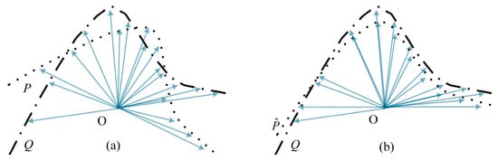
Figure 6. Schematic diagram of the minimum similarity distance. (a) Two characteristic curves that coincide at the centroid; (b) Two characteristic curves that achieve the minimum similarity distance.

As shown in Figure 6b, when $R$ is set to the identity matrix and $A$ to zero vector, the distance vectors $P$ and $Q$ reach their minimum similarity distance. Let the rotated distance vector be $\widehat{P}=\left({\widehat{p}}_1,\cdots {\widehat{p}}_i,\cdots ,{\widehat{p}}_m\right)$. According to Equations (7) and (8), the similarity distance in this case is given by:

$$d\left(\widehat{P},Q,I,0\right)=S_d\left(P,Q\right)$$

(9)

A closer analysis reveals that the absolute value of the difference between the magnitudes of vectors $P$ and $Q$ is subject to the constraint:

$$\left|{\displaystyle \sum _{i=1}^m\Vert p_i\Vert }-{\displaystyle \sum _{i=1}^m\Vert q_i\Vert }\right|=\left|{\displaystyle \sum _{i=1}^m\Vert {\widehat{p}}_i\Vert }-{\displaystyle \sum _{i=1}^m\Vert q_i\Vert }\right|\le {\displaystyle \sum _{i=1}^m\left|\Vert {\widehat{p}}_i\Vert -\Vert q_i\Vert \right|}\le {\displaystyle \sum _{i=1}^m\Vert {\widehat{p}}_i-q_i\Vert }$$

From the Cauchy–Schwarz inequality, together with Equations (7) and (9), we obtain:

$${\displaystyle \sum _{i=1}^m\Vert {\widehat{p}}_i-q_i\Vert }\le \sqrt{m}\sqrt{{\displaystyle \sum _{i=1}^m\Vert {\widehat{p}}_i-q_i{\Vert }^2}}=\sqrt{m}\times \sqrt{m}\times \sqrt{{\displaystyle \frac{1}{m}}{\displaystyle \sum _{i=1}^m\Vert {\widehat{p}}_i-q_i{\Vert }^2}}=m{S}_d\left(P,Q\right)$$

Therefore, the derived Equation (10) can be used for the similarity analysis of unimodal characteristic curves.

$$\left|{\displaystyle \sum _{i=1}^m\Vert p_i\Vert }-{\displaystyle \sum _{i=1}^m\Vert q_i\Vert }\right|\le m{S}_d\left(P,Q\right)$$

(10)

However, Equation (10) has difficulties in similarity analysis. Intersection edge points cannot be detected by adjusting similarity weights. This often leads to misdetection for gradual edge points.

3.3. Mapping Vectors

As shown in Figure 5d, $P=\left(p_1,\cdots p_i,\cdots ,p_m\right)$ is a distance vector containing sampling points. Based on the Mexican Hat wavelet function (Equation (11)), a novel mapping vector $hswt$ is constructed (Equation (12)).

$${\psi }_k(t)={\displaystyle \frac{2}{\sqrt{3k}{\pi }^{1/4}}}\left(1-{\displaystyle \frac{t^2}{k^2}}\right)e^{-{\displaystyle \frac{t^2}{2k^2}}}$$

(11)

$$\left\{\begin{array}{l}hswt(P)=\left[w_1,\cdots ,w_k,\cdots w_d\right]\\ w_k(P)=\gamma {\displaystyle \sum _i^m‖p_i-p_0‖{\psi }_k\left(\frac{i-1}{m}\right)}\end{array}\right.$$

(12)

where $\gamma$ is the coefficient that must satisfy $\gamma >0$, and it is also the scale parameter of the wavelet transform, $d$ is the preset dimension of the mapping vectors and centroid vector of the characteristic curve is $p_0={\displaystyle \raisebox{1ex}{$1$}\!\left/ \!\raisebox{-1ex}{$m$}\right.}{\displaystyle {\sum }_{i=1}^m{p}_i}$. The core idea of $hswt$ is to encode distance vectors using wavelet transforms. At each level, wavelets decompose the spatial relationship between sample points and the centroid, and the resulting values serve as the mapping vector values. The wavelet values from level 1 to $d$ are subsequently concatenated to generate a mapping vector. Moreover, the mapping vectors have two key properties, which significantly enhance their performance in edge detection tasks. In the following, these two properties are formally demonstrated.

Property 1.

Rotation and Translation Invariance.

For a distance vector $P$ and its rigidly transformed counterpart $P^{\prime }$, their values remain unchanged under the $hswt$ mapping. This property ensures the reliability of similarity analysis of characteristic curves using $hswt$.

Let the distance vector $P=\left(p_1,\cdots p_i,\cdots ,p_m\right)$, and define its transformed vector $P^{\prime }=\left({p^{\prime }}_1,\cdots {p^{\prime }}_i,\cdots ,{p^{\prime }}_m\right)$, where ${p^{\prime }}_i=R{p}_i+A$ ($R$ is a rotation matrix and $A$ is a translation matrix).

Proof. 

The centroid of P

$$p_0={\displaystyle \frac{1}{m}}{\displaystyle {\sum }_{i=1}^m{p}_i}$$

The transformed centroid

$${p^{\prime }}_0={\displaystyle \frac{1}{m}}{\displaystyle {\sum }_{i=1}^m\left(R{p}_i+A\right)=R{p}_0+A}$$

Then

$$‖\left(R{p}_i+A\right)-{p^{\prime }}_0‖=‖R{p}_i+A-\left(R{p}_0+A\right)‖=‖R\left(p_i-p_0\right)‖$$

According to the properties of rotation matrices

$$‖R\left(p_i-p_0\right)‖=‖p_i-p_0‖$$

From the construction of Equation (12), it follows that $hswt(P^{\prime })=hswt(P)$. When any rigid transformation is applied to the distance vector $P$, the $hswt(P)$ mapping remains unchanged. This property verifies that the mapping vector represents the shape of characteristic curves by decomposing the distance from the centroid to each sampling point. Since this representation is independent of the initial position of characteristic curves, it eliminates the need for centroid alignment as illustrated in Figure 6a and avoids the process of solving the rotation matrix $R$ when comparing shape similarity. This improves computational efficiency, allowing for faster differentiation between planar points and gradually edge points. □

Property 2.

Distance Consistency.

For vectors $P$ and $Q$, if they have minimum similarity distance $S_d(P,Q)\to 0$ in the Euclidean space, then their $hswt$ mappings satisfy $\left|hswt(P)-hswt(Q)\right|\to 0$. This property ensures the validity of similarity analysis for characteristic curves.

Let the distance vectors $P$ and $Q$. To prove: if $S_d(P,Q)\to 0$, then $\underset{S_d\left(P,Q\right)\to 0}{\lim }\left|hswt(P)-hswt(Q)\right|\to 0$.

Proof. 

For the wavelet at each level

$$\left|w_k\left(P\right)-w_k\left(Q\right)\right|\le \gamma {\displaystyle \sum _{i=1}^m{\psi }_k\left(‖p_i‖-‖q_i‖\right)}\le \gamma {\displaystyle \frac{2}{\sqrt{3k}{\pi }^{1/4}}}{\displaystyle \sum _{i=1}^m\left|‖p_i‖-‖q_i‖\right|}$$

It can be obtained from Equation (10).

$$\gamma {\displaystyle \frac{2}{\sqrt{3k}{\pi }^{1/4}}}{\displaystyle \sum _{i=1}^m\left|‖p_i‖-‖q_i‖\right|}\le \gamma m{\displaystyle \frac{2}{\sqrt{3k}{\pi }^{1/4}}}{S}_d\left(P,Q\right)$$

Therefore

$$\left|w_k(P)-w_k(Q)\right|\le S_d\left(P,Q\right){\displaystyle \frac{C}{\sqrt{k}}}=C{S}_d\left(P,Q\right)g\left(k\right)$$

(13)

In this expression, $C=2\gamma m/\sqrt{3}{\pi }^{1/4}$ is a constant, and $g\left(k\right)=1/\sqrt{k}$.

Since $g\left(k\right)>0$, $C\ge 0$, Equation (14) can be deduced from Equation (13).

$$\underset{S_d\left(P,Q\right)\to 0}{\lim }\left|hswt(P)-hswt(Q)\right|\to 0$$

(14)

This property indicates that the distance between characteristic curves in the Euclidean space is positively correlated with the corresponding distance in the mapping vector space. Therefore, if two characteristic curves are similar in the Euclidean space, they remain similar in the mapping space. Based on this relationship, the scalability of the mapping vector space (different levels of wavelet transform) can be used to distinguish between planar points and slow-varying edge points. □

Definition of $COWT$: $COWT$ is a wavelet transform-based similarity judgment function. It assesses whether characteristic curves (represented by distance vectors) meet similarity conditions within a given scale range. Its mathematical definition is as follows:

Definition 1.

Given two distance vectors $P$  and $Q$, a preset wavelet decomposition level $d$, and the similarity threshold $\tau$, the $COWT$ function is defined as follows:

$$COWT(P,Q,d,\tau )=\left\{\begin{array}{cc}\mathrm{True},\hfill & \mathrm{if} \forall k\in \{1,2,\dots ,d\},\left|w_k(P)-w_k(Q)\right|\le \tau \cdot g(k)\hfill \\ \mathrm{False},\hfill & \mathrm{otherwise}\hfill \end{array}\right.$$

(15)

$w_k\left(P\right)$ and $w_k\left(Q\right)$ denote the mapping values of distance vectors $P$ and $Q$ under the k-th level wavelet transform, respectively, with the specific calculation method detailed in Equation (12). Furthermore, $g\left(k\right)=1/\sqrt{k}$.

Corollary 1.

Since $g\left(k\right)>0$, if $COWT\left(P,Q,d,\tau \right)$ does not hold for a wavelet transform at a certain level $k$, then $C{S}_d\left(P,Q\right)>\tau$.

Therefore, for two characteristic curves characterized by distance vectors $P$ and $Q$, choosing wavelet transforms at different levels affects the outcome of similarity assessment. When a low-level wavelet is employed (e.g., k = 1), its broader waveform allows the difference between their mapping vectors to remain within a larger tolerance threshold $\tau$. Local feature differences between and are smoothed, resulting in high similarity. However, as the wavelet level approaches infinity, the mapping vectors must be exactly equal to be considered similar. According to Equation (16), $hswt(P)=hswt(Q)$. Consequently, even minor differences between $P$ and $Q$ are amplified, leading to a significant reduction in similarity.

$$\underset{k\to \infty }{\lim }\tau g\left(k\right)=\underset{k\to \infty }{\lim }{\displaystyle \frac{\tau }{\sqrt{k}}}=0$$

(16)

$COWT\left(P,Q,d,\tau \right)$ exhibits scale monotonicity. A smaller $k$ value corresponds to a looser similarity condition. A larger $k$ value corresponds to a stricter similarity condition. If the condition in Equation (15) is not satisfied at the k-level wavelet scale, it will not hold at any larger scale. Thus, there is no need to compute the $S_d$ parameter. Planar points and gradual edge points can be distinguished by adjusting $\tau$ and $d$. Specifically, the centroids of all characteristic curves are clustered using DBSCAN. Several clusters are formed. In each cluster, the Euclidean distance between each sample and the cluster mean is computed. The point closest to the mean is selected. Its characteristic curve is taken as the standard template. This ensures that the template represents the typical characteristics of the cluster. Finally, Algorithm 1 is applied for similarity matching within each cluster. By checking the $COWT\left(P,Q,d,\tau \right)$ condition from level 1 to level $d$, all qualified edge points are identified. Notably, in this study, experiments on conical shell point clouds confirm that an optimal balance between discriminative power and stability is achieved when the wavelet scale parameter $k$ ranges from 1 to $d$, with the mapping dimension $d$ fixed at 4. This parameter choice aligns with established practices in 2D image processing [19] and wavelet signal decomposition theory [20]. Typically, employing 3 to 6 wavelet scale levels suffices to capture meaningful multi-scale features. Furthermore, the parameter $\tau$ adopted as an empirical constant, conventionally assumes values within the interval [0.1, 1].

Algorithm 1. Similarity search

Input: $hswt(P)$$\mathrm{the} \mathrm{standard} \mathrm{mapping} \mathrm{vector}; Q_i$ candidate distance vectors; $\tau$ threshold parameter; level $d$ Output: the distance vectors of edge points Steps: For each candidate distance vector set $Q_i$$(\mathrm{where} i=1$ to $j$), do Compute $hswt(Q_i)$ For $k=1$ to $d$ do If $\left|w_k(P)-w_k(Q)\right|\ge \tau g\left(k\right)$ then Break $(\mathrm{terminate} \mathrm{checking} \mathrm{for} Q_i$$\mathrm{and} \mathrm{proceed} \mathrm{to} \mathrm{next} Q_{i+1}$) End if End for If $COWT\left(P,Q,d,\tau \right)$ is satisfied, then output $Q_i$ End if End for

4. Experiments and Results

This section verifies the feasibility of the proposed point cloud edge detection method. The experiments include three parts: gradual edge detection, multi-type edge detection, and point cloud registration. The results show that the method can accurately detect different types of edges in point clouds from different data sources. In addition, it achieves high detection accuracy in point cloud registration experiments.

4.1. Evaluation Indicators

The performance of edge detection is evaluated using three metrics: precision, recall, and F1 score [6].

Precision: Precision measures the reliability of the detection results. It is defined as the proportion of true edge points among all points detected as edges. It is calculated as follows.

$$precision={\displaystyle \frac{N_e}{N_s}}$$

(17)

$N_e$ denotes the number of correctly detected edge points, and $N_s$ represents the total number of edge points predicted by the algorithm. A high precision indicates that the algorithm produces fewer false detections and yields results with higher confidence.

Recall: Recall evaluates the algorithm’s ability to cover the true edges. It is defined as the proportion of true edges that are correctly detected. It is calculated as follows.

$$recall={\displaystyle \frac{N_e}{N_T}}$$

(18)

$N_e$ denotes the number of correctly detected edge points, and $N_T$ represents the total number of true edge points. A high recall indicates that the algorithm can effectively capture the true edge structure and reduce missed detections.

F1 score: The F1 score measures the balance between precision and recall. it is defined as their harmonic mean. It is calculated as follows.

$$F_1=2\times {\displaystyle \frac{precision\cdot recall}{precision+recall}}$$

(19)

The value closer to 1 indicates a better trade-off between reducing false detections and missed detections, as well as a stronger ability to preserve the integrity of edge structures.

4.2. Results of Gradual Edge Detection

To evaluate the performance of detecting gradual edge points, the elliptical cylindrical point cloud models with different curvatures were generated on the MATLAB 2024a platform. Each model contains 18,000 points. This simulation used random sampling without adding noise. Random sampling mimics the phenomenon of irregular distribution of points within point clouds in real laser scanning. The absence of noise creates a controlled setting, similar to high-quality scan data. This allows the evaluation to focus mainly on the core challenge of curvature variation.

The major axis generatrix was selected as the primary edge detection region (see Figure 7). The truth edge points were rigorously defined as points precisely located on the parametric curve of the major-axis generatrix, which traces the trajectory of the semi-major axis endpoints along the height of the cylinder. For the quantitative evaluation of precision and recall, a detected point was classified as a true positive if its 3D Euclidean distance to this parametric curve did not exceed 0.15 units. In this section, the EA algorithm [16], which is also based on PCA, was chosen for comparison. A systematic evaluation and comparative analysis were conducted to assess the performance of the proposed method on gradual edge points with different curvatures.

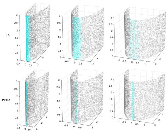
Figure 7. Edge detection results of different algorithms.

The parameters of the elliptical cylinder were set as follows: the height was fixed at 3 units, and the major axis radius was kept constant at 3 units. Different gradual edge curvatures were generated by adjusting the minor axis radius to 0.5, 1.0, and 1.5 units. The results (Figure 7) show that, as the minor axis radius increases (i.e., as the edge points curvature increases), the detection performance of the EA algorithm drops significantly. The detected edge lines become blurred and fractured. The detection range also shows abnormal diffusion, and non-edge regions are even misidentified as edges. In contrast, the proposed algorithm (denoted as PCHA) demonstrates superior edge detection performance. Clear edge lines are preserved in the results, even when the minor axis radius increases to 1.5 units.

As shown in Table 1, when the minor axis parameter is set to 0.5, the EA algorithm achieves a recall of 0.9138 in point cloud edge detection, but its precision is only 0.5208. This suggests that EA enhances recall by broadening the criteria for target recognition, which comes at the cost of reduced precision.

Table 1. Index results of edge detection of elliptical cylinders under different minor axes. The direction of the arrow indicates the tendency for that metric to get better.

Length of the Minor Axis	EA			PCHA
	Precision ↑	Recall ↑	F1 ↑	Precision ↑	Recall ↑	F1 ↑
0.5	0.5208	0.9138	0.6635	0.9117	0.9256	0.9186
1	0.3872	0.7324	0.5066	0.9028	0.9137	0.9082
1.5	0.2342	0.5356	0.3259	0.8913	0.9023	0.8968

To better illustrate the influence of parameter variation on algorithm performance, Figure 8 compares EA and PCHA under different minor-axis lengths. Figure 8a shows that, as edge curvature increases, the precision of EA drops significantly, while PCHA remains stable. Figure 8b shows that, at low curvature, the recall of both algorithms is comparable. However, as curvature increases, EA suffers a marked decline, while PCHA remains nearly stable. Figure 8c further demonstrates that PCHA preserves edge structure integrity much better than EA. In summary, these experiments provide strong evidence that the PCHA algorithm achieves superior performance in detecting gradual edge points.

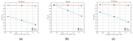
Figure 8. Performance comparison between EA and PCHA under varying minor axis length: (a) Precision, (b) Recall, (c) F1 score.

4.3. Results of Multi-Type Edge Detection

The study employed both a self-constructed experimental dataset and the publicly available ModelNet40 dataset from Princeton University. The performance of multi-type edge detection was analyzed from both quantitative and qualitative perspectives.

Figure 9 shows the laser scanning platform for conical workpieces built in this study. The system consists of a rotary table, a laser scanner (Figure 10), an inverter, and a computer. Under the unified control of the computer, the laser scanner captures the surface of rotating conical shells (Figure 11 and Figure 12), thereby generating the local experimental dataset. The acquired point clouds contain 46,223 points for the second-order conical shell and 31,008 points for the third-order conical shell, with an average point spacing ranging from 0.2 mm to 0.3 mm in physical scale. The noise in the point clouds primarily arises from mechanical vibration during scanning, leading to non-uniform point density, as well as drift points caused by the required rotational motion. Prior to analysis, preprocessing steps were applied: statistical outlier removal (SOR) was used to remove isolated noise points, and voxel grid down-sampling was performed to ensure consistent point density across the dataset.

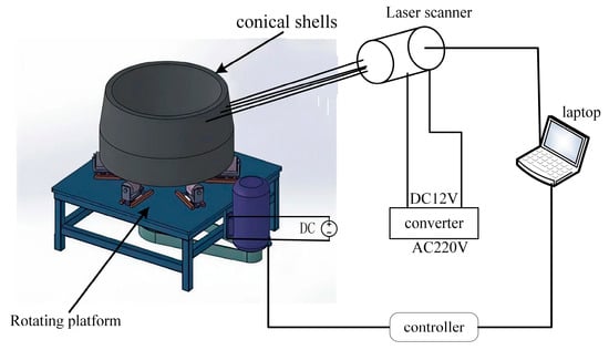
Figure 9. Point cloud data acquisition platform for conical shells.

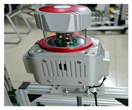
Figure 10. Model RIEGL_VUX-1-22 laser scanner.

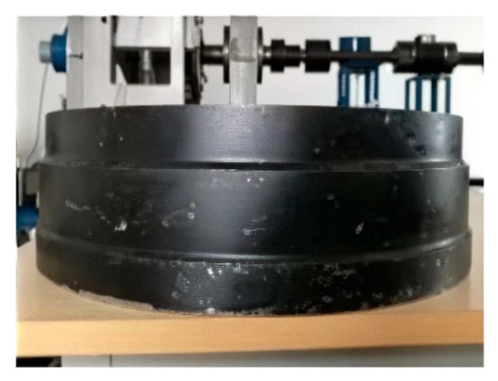
Figure 11. Third-order conical shell.

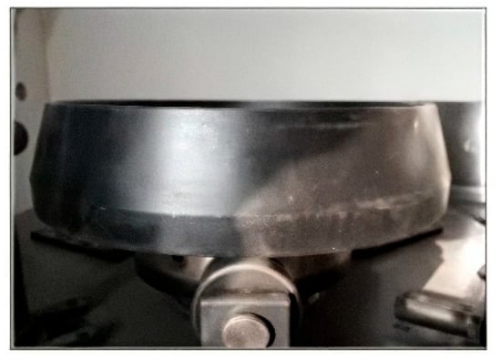
Figure 12. Second-order conical shell.

To further verify the generality of the algorithm, representative models were selected from the ModelNet40 dataset for comparison. This dataset, released by Princeton University, contains 40 categories of 3D models, including airplanes, cars, and factories. Considering the need to identify both complex and gradual edge features, the bottle and bowl models were selected as representative test objects. These models exhibit gradual edge transitions and open boundary regions that closely resemble the geometric characteristics of industrial conical shell structures. Their compound surface features, such as curved walls and smooth joint transitions, simulate typical deformation or weld regions found in conical shells. Therefore, these models effectively represent the structural complexity of real process equipment and enhance the generalization and engineering relevance of the proposed edge detection method. In terms of data preparation, the CAD meshes from ModelNet40 were converted into point clouds using uniform Poisson disk sampling to ensure a spatially balanced distribution of points, with each model containing approximately 10,000 points to preserve geometric details while maintaining computational efficiency. Subsequently, all point clouds were normalized into a unit sphere by first translating their centroids to the coordinate origin and then uniformly scaling them so that the farthest point from the origin had a distance of one. This scale and position normalization places all models within a consistent spatial frame of reference.

4.3.1. Quantitative Analysis

In this section, three representative methods were selected for comparison: EA [16] based on local neighborhood geometry, DNG [10] based on surface transformation, and GFR [11] based on graph representation.

Table 2 reports the results with three evaluation metrics. All methods were tuned with their optimal parameter settings on each dataset to ensure a fair comparison. The EA algorithm showed the weakest overall performance on the ring forging dataset. For the second-order conical shell and third-order conical shell test sets, their key metrics were significantly lower than the baseline. Notably, its edge extraction ability degraded severely in the bowl model test. The DNG algorithm performed better than EA but still showed a clear gap from the expected performance. In the conical shell dataset, GFR achieved the second-best performance, only behind PCHA. For models with gradual features, such as bottles and bowls, PCHA exhibited significant advantages. Its F1 scores reached 0.7987 and 0.8384, representing improvements of 12.29% and 20.09% over the second-best method, GFR.

Table 2. Results of edge detection metrics. The arrow indicates the direction of improvement for each metric. The best results are highlighted in bold.

Dataset name	Metrics Model	Precision ↑	Recall ↑	F1 ↑
second-order conical shell	EA	0.4037	0.4394	0.4208
	DNG	0.5853	0.6034	0.5942
	GFR	0.7083	0.7168	0.7125
	PCHA	0.7641	0.7721	0.7681
third-order conical shell	EA	0.3017	0.3828	0.3374
	DNG	0.5264	0.5436	0.5349
	GFR	0.6735	0.6883	0.6808
	PCHA	0.7441	0.7637	0.7538
bottle	EA	0.3843	0.4065	0.3951
	DNG	0.6076	0.6482	0.6272
	GFR	0.6543	0.6987	0.6758
	PCHA	0.7856	0.8123	0.7987
bowl	EA	0.2032	0.2396	0.2199
	DNG	0.3955	0.4128	0.4040
	GFR	0.6258	0.6497	0.6375
	PCHA	0.8237	0.8536	0.8384

4.3.2. Qualitative Analysis

In this section, qualitative comparison experiments on edge detection were conducted using both the self-constructed point clouds dataset and the ModelNet40 dataset. The methods compared include EA, DNG, GFR, and the proposed PCHA. As shown in Figure 13, the original point cloud models are displayed as opaque objects. In the detection results, non-edge regions are set to 10% transparency, and detected edge points are highlighted in blue.

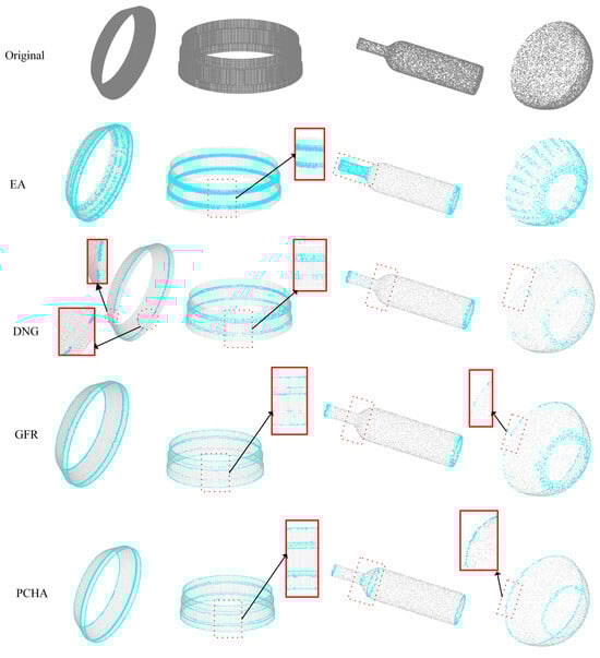
Figure 13. Qualitative results of edge detection by different algorithms for the second-order conical shell, third-order conical shell, bottle, and bowl.

For the second-order conical shell, EA missed the upper ring edge and produced large-scale false detections. DNG generated discontinuous edge lines. While GFR detected all edges, the continuity in the middle was poor. In contrast, PCHA clearly identified all edges. For the more complex third-order conical shell model, the compact spacing of middle edges led EA and DNG to fail in recognizing the upper and lower open boundaries. GFR detected edge lines but with numerical deviations. PCHA accurately detected all six edge lines. For the bottle model with gradual features, EA misclassified the entire bottle mouth as an edge. DNG and GFR detect the edge points at the bottle mouth and bottom but fail to capture the gradual edge points along the bottle body. PCHA successfully detected all edges, including the gradual edge of the bottle body. For the bowl model, EA and DNG completely failed at the open boundaries of the bowl mouth. GFR detected partial edges, but with severe discontinuities. PCHA detected relatively complete and continuous edge lines at both the bowl mouth and the base. PCHA effectively addressed the challenges of missed and false detections on gradual edge points. Moreover, the algorithm did not degrade detection performance on open boundaries and sharp edge regions. PCHA proves capable of reliably detecting multiple types of edges.

4.4. Registration Experiment

Since condition evaluation based on point cloud registration depends critically on reliable edge information, the accuracy of edge extraction directly influences the robustness of process safety assessment. To quantitatively analyze how different edge detection strategies affect registration performance, we conduct systematic experiments using both the Princeton public dataset and self-acquired point cloud data. In the experiment, point cloud registration was performed by applying the ICP algorithm to EA, DNG, GFR, LMAGD [6] and PCHA, respectively. To eliminate bias from initial pose differences, we strictly fix the initial translation and rotation parameters across all registration experiments. For the ICP algorithm, we calculate the point cloud registration error according to Equation 20 after each iteration and continue iterating until the error change is below the preset threshold (10⁻⁵ in the experiment). The final errors in Table 3 correspond to the stable values at the convergence points. This ensures that the reported point cloud registration errors reflect algorithmic performance rather than inconsistent pose initialization or insufficient iteration. In theory, high-precision registration should yield complete overlap between homologous point cloud models. Otherwise, significant mismatches will occur. To enable quantitative comparison of registration performance, the following point cloud registration error metrics are defined.

$$\epsilon =\sqrt{{\displaystyle \frac{{\displaystyle \sum _{i=1}^k{(X_i-{X^{\prime }}_i)}^2}}{k}}}$$

(20)

Table 3. Point cloud registration errors of different edge detection algorithms (Units: mm).

Dataset Name	EA	DNG	GFR	LMAGD	PCHA
second-order conical shell	94.8683	37.4165	1.7416	1.6742	0.8591
Third-order conical shell	45.8257	17.3205	3.8326	1.9836	0.6449
bottle	22.0227	8.6441	4.3748	3.3743	0.0674
bowl	64.5290	36.1801	9.7485	10.7439	0.0316

Here, $X_i$ denotes the minimum distance between the source and target point clouds prior to each iteration of the ICP registration algorithm. ${X^{\prime }}_i$ denotes the corresponding minimum distance after each iteration. The “minimum distance” refers to the Euclidean distance between corresponding point pairs, where correspondences are established by a k-d tree-assisted nearest neighbor search from the source to the target point cloud.

To clearly illustrate the variation trends in Table 3, registration error curves are plotted in Figure 14. Considering the large differences in the magnitude of the raw data, the vertical axis is log-scaled with base 10 to enhance visualization and balance the trend features across different ranges. Notably, the experimental dataset comprises four types of objects with varying geometries and dimensions: a second-stage conical shell (maximum diameter 315.2 mm), a third-stage conical shell (maximum diameter 380.3 mm), a bottle (maximum diameter 60 mm), and a bowl-shaped object (maximum diameter 120 mm).

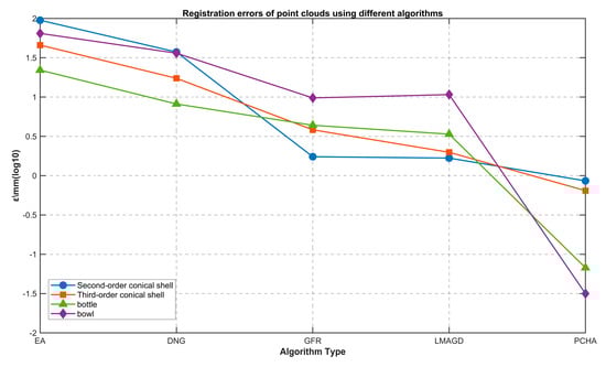
Figure 14. The errors of point cloud registration accuracy of each algorithm.

As shown in Figure 14, the registration errors of the PCHA algorithm are consistently lower than those of existing methods across all cases. The improvement is particularly significant for bottle and bowl models with gradual features. These errors correspond to remarkably small proportions of the nominal maximum diameters: the error of the second-order conical shell accounts for approximately 0.2726% of its maximum diameter, the third-order conical shell’s error is about 0.1696%, the bottle’s error makes up roughly 0.112%, and the bowl’s error is merely around 0.0263% of its maximum diameter. For context, errors from competing algorithms (e.g., EA, DNG, GFR, LMAGD in Table 3) often exceed 1% of the nominal maximum diameter for these datasets (e.g., EA’s error for the second-order conical shell reaches 94.8683 mm, accounting for 30.1% of its maximum diameter), further emphasizing PCHA’s edge detection superiority. Its unique mechanism effectively captures gradual edge points that other methods miss, minimizing registration errors.

The five sets of comparative results in Figure 15a–d show that the EA algorithm produces significant registration errors, followed by the DNG algorithm. The GFR and LMAGD algorithm demonstrates relatively better performance on the conical shell model but exhibits a marked decline in accuracy on the bottle and bowl models. In contrast, the PCHA algorithm consistently achieves the best registration performance across all test models, with notable advantages on bottle and bowl models with gradual features.

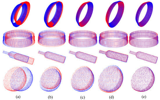
Figure 15. Different algorithm registration results. (a) EA, (b) DNG, (c) GFR, (d) LMAGD, (e) PCHA.

5. Discussion

In this experiment, the point clouds obtained through laser scanning of the self-constructed conical shell inherently contain typical scanning noise. For example, the uneven density of the point cloud results from mechanical vibration during the measurement of the conical shell, and the drift points arise from the rotation required in the measurement process. The robustness of the PCHA method under such conditions primarily stems from the redundancy of characteristic curves. This redundancy enables the extraction of accurate geometric information within the radial range and mitigates the impact of local disturbances. Although the proposed method performs well in the experiment, its edge point classification model relies on the results of PCA calculations, which may limit its performance under extreme noise conditions. While such extreme noise is not the dominant case in the test dataset of this study, it represents certain extreme working scenarios. Future research can be extended in the following two directions: First, further investigate the adaptability and robustness of the method under systematically controlled noisy conditions. Second, explore the integration of deep learning techniques to improve the accuracy and efficiency of edge detection.

6. Conclusions

This study proposes a point cloud edge detection algorithm. The method applies pattern recognition to characteristic curves derived from the ratio of PCA eigenvalues to build a classification model for edge points. In this way, it detects open boundaries and most sharp edge points in point cloud models. To address the challenge of distinguishing planar points and gradual edge points, distance vectors of the characteristic curves are first defined. Wavelet transforms are then applied to the distance vectors to generate mapping vectors. Finally, the unique properties of the mapping vectors enable accurate discrimination of edge points with different curvatures. The main conclusions are as follows:

(1)

The PCHA algorithm shows strong performance in detecting gradual edge points. In the elliptical cylinder experiment with a minor axis radius of 1.5, it achieves a detection precision of 0.8913 and a recall of 0.9023.

(2)

The PCHA algorithm demonstrates good detection accuracy and generalization. On both the local dataset and the ModelNet40 benchmark, its F1 score exceeds that of the second-best GFR algorithm, achieving an average improvement percentage of 12.73%.

(3)

The PCHA algorithm improves the performance of edge detection. In point cloud registration experiments across different models, it consistently yields the lowest registration errors. It provides an effective assessment method for the inconsistency between the workpiece’s edge quality and its overall integrity.

In summary, the proposed algorithm can effectively identify edge points of conical workpieces.

References

- Dai, Z.; Qiao, H.; Hao, X.; Wang, Y.; Lei, H.; Cui, Z. Influence of Heterogeneous Foundation on the Safety of Inverted Cone Bottom Oil Storage Tanks under Earthquakes. Buildings 2023, 13, 1720. [Google Scholar] [CrossRef]
- Stoicescu, A.-A.; Ripeanu, R.G.; Tănase, M.; Ilincă, C.N.; Toader, L. Multifactorial Analysis of Defects in Oil Storage Tanks: Implications for Structural Performance and Safety. Processes 2025, 13, 2575. [Google Scholar] [CrossRef]
- Stoicescu, A.-A.; Ripeanu, R.G.; Tănase, M.; Toader, L. Current Methods and Technologies for Storage Tank Condition Assessment: A Comprehensive Review. Materials 2025, 18, 1074. [Google Scholar] [CrossRef] [PubMed]
- Pallas Enguita, S.; Chen, C.-H.; Kovacic, S. A Review of Emerging Sensor Technologies for Tank Inspection: A Focus on LiDAR and Hyperspectral Imaging and Their Automation and Deployment. Electronics 2024, 13, 4850. [Google Scholar] [CrossRef]
- Makka, A.; Pateraki, M.; Betsas, T.; Georgopoulos, A. Detecting Three-Dimensional Straight Edges in Point Clouds Based on Normal Vectors. Heritage 2025, 8, 91. [Google Scholar] [CrossRef]
- Ma, F.F.; Zhang, Y.; Chen, J.T.; Qu, C.Z.; Huang, K. Edge detection for 3D point clouds via locally max-angular gaps descriptor. Meas. Sci. Technol. 2024, 35, 025207. [Google Scholar] [CrossRef]
- Bode, L.; Weinmann, M.; Klein, R. BoundED: Neural boundary and edge detection in 3D point clouds via local neighborhood statistics. ISPRS J. Photogramm. Remote Sens. 2023, 205, 334–351. [Google Scholar] [CrossRef]
- Daniels, J.; Ochotta, T.; Ha, L.K.; Silva, C.T. Spline-based feature curves from point-sampled geometry. Visual Comput. 2008, 24, 449–462. [Google Scholar] [CrossRef]
- Yutaka, O.; Alexander, B.; Hans-Peter, S. Ridge-valley lines on meshes via implicit surface fitting. ACM Trans. Graph. 2004, 23, 609–612. [Google Scholar] [CrossRef]
- Demarsin, K.; Vanderstraeten, D.; Volodine, T.; Roose, D. Detection of closed sharp edges in point clouds using normal estimation and graph theory. Comput. Aided Des. 2007, 39, 276–283. [Google Scholar] [CrossRef]
- Chen, S.H.; Tian, D.; Feng, C.; Vetro, A.; Kovacevic, J. Fast Resampling of Three-Dimensional Point Clouds via Graphs. IEEE T Signal Proces. 2018, 66, 666–681. [Google Scholar] [CrossRef]
- Qi, J.K.; Hu, W.; Guo, Z.M. Feature Preserving and Uniformity-Controllable Point Cloud Simplification on Graph. IEEE Int. Con. Multi. 2019, 284–289. [Google Scholar] [CrossRef]
- Deng, Q.W.; Zhang, S.Y.; Ding, Z. Point Cloud Resampling via Hypergraph Signal Processing. IEEE Signal Proc. Let. 2021, 28, 2117–2121. [Google Scholar] [CrossRef]
- Xia, S.B.; Wang, R.S. A Fast Edge Extraction Method for Mobile Lidar Point Clouds. IEEE Geosci. Remote Sens. Lett. 2017, 14, 1288–1292. [Google Scholar] [CrossRef]
- Zhang, Y.H.; Geng, G.H.; Wei, X.R.; Zhang, S.L.; Li, S.S. A statistical approach for extraction of feature lines from point clouds. Comput. Graph. 2016, 56, 31–45. [Google Scholar] [CrossRef]
- Dena, B.; Josep, R.C.; Javier, R.-H. Fast and Robust Edge Extraction in Unorganized Point Clouds. In Proceedings of the 2015 International Conference on Digital Image Computing: Techniques and Applications (DICTA), Adelaide, Australia, 23–25 November 2015. [Google Scholar] [CrossRef]
- Pauly, M.; Keiser, R.; Gross, M. Multi-scale feature extraction on point-sampled surfaces. Comput. Graph. Forum 2003, 22, 281–289. [Google Scholar] [CrossRef]
- Quentin, M.; Maks, O.; Leonidas, J.G. Voronoi-Based Curvature and Feature Estimation from Point Clouds. IEEE Trans. Vis. Comput. Graph. 2011, 17, 743–756. [Google Scholar] [CrossRef]
- Maksimović, V.; Lekic, P.; Petrovic, M.; Jakšić, B.; Spalevic, P. Experimental analysis of wavelet decomposition on edge detection. Proc. Est. Acad. Sci. 2019, 68, 284. [Google Scholar] [CrossRef]
- Silik, A.; Noori, M.; Altabey, W.A.; Ghiasi, R. Selecting optimum levels of wavelet multi-resolution analysis for time-varying signals in structural health monitoring. Struct. Control. Health Monit. 2021, 28, 2762. [Google Scholar] [CrossRef]
Disclaimer/Publisher’s Note: The statements, opinions and data contained in all publications are solely those of the individual author(s) and contributor(s) and not of MDPI and/or the editor(s). MDPI and/or the editor(s) disclaim responsibility for any injury to people or property resulting from any ideas, methods, instructions or products referred to in the content. |
© 2026 by the authors. Licensee MDPI, Basel, Switzerland. This article is an open access article distributed under the terms and conditions of the Creative Commons Attribution (CC BY) license.