Abstract
The study focuses on the design of an intelligent information-control system (ICS) for metallurgical production, aimed at robust forecasting of technological parameters and automatic self-adaptation under noise, anomalies, and data drift. The proposed architecture integrates a hybrid LSTM–DNN model with low-discrepancy hypercube sampling using Sobol and Halton sequences to ensure uniform coverage of operating conditions and the hyperparameter space. The processing pipeline includes preprocessing and temporal synchronization of measurements, a parameter identification module, anomaly detection and correction using an ε-threshold scheme, and a decision-making and control loop. In simulation scenarios modeling the dynamics of temperature, pressure, level, and flow (1 min sampling interval, injected anomalies, and measurement noise), the hybrid model outperformed GRU and CNN architectures: a determination coefficient of R2 > 0.92 was achieved for key indicators, MAE and RMSE improved by 7–15%, and the proportion of unreliable measurements after correction decreased to <2% (compared with 8–12% without correction). The experiments also demonstrated accelerated adaptation during regime changes. The scientific novelty lies in combining recurrent memory and deep nonlinear approximation with deterministic experimental design in the hypercube of states and hyperparameters, enabling reproducible self-adaptation of the ICS and increased noise robustness without upgrading the measurement hardware. Modern metallurgical information-control systems operate under non-stationary regimes and limited measurement reliability, which reduces the robustness of conventional forecasting and decision-support approaches. To address this issue, a hybrid LSTM–DNN architecture combined with low-discrepancy hypercube probing and anomaly-aware data correction is proposed. The proposed approach is distinguished by the integration of hybrid neural forecasting, deterministic hypercube-based adaptation, and anomaly-aware data correction within a unified information-control loop for non-stationary industrial processes.
1. Introduction
Modern metallurgical production operates under multidimensional nonlinear dynamics, stochastic disturbances, and incomplete measurement information. For information-control systems (ICSs), this necessitates the simultaneous solution of three interconnected tasks: ensuring the reliability of technological data, implementing adaptive real-time control, and supporting well-grounded decision-making across different levels of the operational hierarchy. A critical limitation remains the processing of rapidly updating data streams while maintaining stability and interpretability of decisions under noise, anomalies, and drifting signal statistics [1].
The integration of artificial intelligence, cloud computing, and the Industry 4.0 paradigm has led to the emergence of intelligent ICS platforms that combine SCADA, ERP, and AI modules for large-scale data analysis and predictive control [2,3]. Neural network models, predictive analytics, and digital twins are increasingly used to improve dispatching efficiency, optimize resource consumption, and reduce technological losses. However, most practical solutions rely either on static deep neural networks (DNNs, CNNs) or on recurrent architectures without a clearly formalized self-adaptation procedure. Such models are sensitive to hyperparameter selection, adapt poorly to regime changes, and often fail to exhibit sufficient noise robustness when confronted with corrupted or anomalous data [4].
These limitations are particularly acute in metallurgy, where technological objects exhibit strong nonlinearity, delays, multivariable coupling, and high cost of control errors [5]. Under such conditions, hybrid intelligent models are required; these are models that simultaneously capture temporal dependencies and multidimensional nonlinear relationships among process parameters, and that additionally include built-in mechanisms for adaptation and control of measurement reliability. The absence of a formal loop for anomaly detection and correction leads to error accumulation, degradation of forecasting accuracy, and reduced robustness of closed-loop control systems.
This work proposes an integrated methodology for designing ICS in metallurgical production, combining a hybrid LSTM–DNN architecture with low-discrepancy hypercube sampling (Sobol/Halton sequences) and a data reliability control module. Low-discrepancy experimental design across operating conditions and hyperparameters ensures uniform coverage of the search domain and reproducible model self-adaptation, while an ε-threshold anomaly-detection and correction loop reduces the proportion of unreliable measurements entering the control circuits. As a result, the system achieves improved forecasting accuracy, noise tolerance, and adaptive capability without requiring upgrades to the existing measurement infrastructure.
While low-discrepancy sequences such as Sobol and Halton have been extensively studied in numerical integration, uncertainty quantification, and classical design of experiments, their application in metallurgical information-control systems remains limited. Existing studies primarily employ these sequences for offline parameter sampling or static optimization tasks. In contrast, the proposed approach integrates low-discrepancy hypercube probing directly into a closed-loop intelligent information-control system, where LD-based sampling is used not only for hyperparameter tuning, but also for adaptive model reconfiguration and data reliability control under regime changes. This coupling of deterministic hypercube coverage with online anomaly detection and correction constitutes the main methodological novelty of the present work in the context of metallurgical process control.
Although LSTM and DNN architectures are well established in the literature [5], the originality of the proposed approach lies not in the individual model components, but in their systematic integration within an adaptive information-control framework. The proposed methodology combines hybrid LSTM–DNN forecasting with low-discrepancy hypercube probing and an explicit reliability-aware correction mechanism, forming a closed-loop architecture designed for non-stationary metallurgical processes. This integration enables adaptive model reconfiguration, online reliability assessment, and proactive decision support, which are not addressed simultaneously in conventional hybrid neural network approaches.
1.1. Background and Related Work
The development of the Industry 4.0 paradigm has significantly accelerated the adoption of data-driven approaches in industrial information and control systems (ICSs), particularly within the framework of cyber–physical systems and digital twins. Digital twins rely on the continuous acquisition and processing of time-series data to enable state estimation, forecasting, and decision support for complex industrial processes. In such systems, the reliability and stability of predictive information play a critical role, as erroneous or unstable forecasts may directly affect control actions and lead to increased technological risks and economic losses [6].
Neural network-based models are widely used for forecasting industrial process variables due to their ability to capture nonlinear relationships and temporal dependencies. Recurrent neural networks, including Long Short-Term Memory (LSTM) and Gated Recurrent Unit (GRU) architectures, as well as convolutional neural networks (CNNs), have demonstrated strong performance in modeling complex dynamic behavior of technological objects and are frequently integrated into digital twin and predictive analytics frameworks. However, most existing studies primarily focus on improving prediction accuracy under stationary or weakly varying operating conditions. Issues related to model adaptability, robustness to regime changes, and sensitivity to noisy or corrupted measurements are often insufficiently addressed [7].
In addition to prediction accuracy, the assessment of prediction reliability and anomaly detection has become an important research direction. In real industrial environments, sensor degradation, measurement errors, communication delays, and unexpected disturbances are unavoidable. Nevertheless, in many existing approaches, anomaly detection and reliability evaluation are treated as auxiliary or offline procedures, separated from the forecasting process itself. As a result, control systems may operate based on predictions whose uncertainty is not explicitly quantified, reducing the robustness of closed-loop control and increasing the risk of error accumulation [8].
Recent studies emphasize the need for integrated architectures that combine forecasting, adaptability, and reliability assessment within a unified framework. In this context, the proposed approach differs from existing methods by integrating neural network-based forecasting with low-discrepancy hypercube sampling and an explicit reliability control mechanism. Unlike conventional applications of low-discrepancy sequences limited to offline optimization or static experimental design, the proposed architecture embeds deterministic hypercube probing into an adaptive information-control loop [9]. This integration enables systematic exploration of operating conditions, online model reconfiguration, and identification of unreliable measurements, thereby extending existing approaches and enhancing their applicability to real-world metallurgical ICS.
Beyond single-domain forecasting, recent research has increasingly addressed cross-domain reliability prediction via transfer learning and federated learning paradigms, particularly in machinery fault diagnosis and predictive maintenance [10]. Federated transfer learning (FTL) has been surveyed as a privacy-preserving mechanism to transfer diagnostic knowledge across distributed assets and operating domains, while remaining useful life (RUL) studies have proposed GRU-based memory enhancements to improve degradation modeling under varying conditions [11]. In parallel, distribution discrepancy metrics have been introduced to explicitly handle time-varying domain shifts in transfer diagnosis [12]. Although these approaches demonstrate strong cross-domain generalization, they typically assume the availability of transferable representations across domains and/or federated optimization infrastructure, which may be difficult to ensure in metallurgical information-control systems due to strict real-time constraints, data confidentiality, and strong process specificity. Therefore, this study focuses on improving reliability and robustness within a single-domain industrial setting by integrating hybrid LSTM–DNN forecasting with low-discrepancy hypercube probing and an explicit anomaly-aware reliability control mechanism, without relying on cross-domain data transfer or federated training.
1.2. Motivation and Problem Statement
Metallurgical information-control systems operate under conditions of complex process dynamics, frequent regime changes, and limited reliability of measurement data. These factors significantly complicate forecasting, monitoring, and decision-support tasks, especially when classical model-based or rule-based approaches are applied. In industrial practice, such approaches often exhibit limited adaptability to non-stationary behavior and sensor disturbances, which motivates the development of data-driven and hybrid architectures capable of operating robustly under changing technological conditions.
The proposed architecture of the information and control system (ICS) is based on the modular principle and includes the following key components:
- Data acquisition and preprocessing module. This module receives raw signals from process sensors and preprocesses them. During preprocessing, the data is filtered of noise, normalized to scale, and brought to a standard time scale (time-synchronized). The output is a cleaned, time-coordinated multichannel dataset ready for further analysis. The preprocessed data are then sent both to the parametric identification block and directly to the predictive model.
- Parametric identification block. In this block, the dynamic identification of the controlled object’s (metallurgical unit) current characteristics is performed. Based on incoming cleaned data, approximation and stochastic state estimation are performed, allowing the determination of key process parameters in real time. In essence, the module calculates the actual object model parameters (e.g., coefficients, time constants, etc.) that reflect changing process conditions. The results of parametric identification can be used to adjust the model or control algorithms; for example, it can be used to update the internal parameters of the hybrid neural network or adapt control rules as the dynamics of the object change.
- Hypercube probing algorithm (LD-sequencing). To optimize system performance, a special configuration brute-force algorithm that probes the parameter hypercube using low-dispersed sequences (LD sequences), such as Sobol or Halton sequences, is used. This module generates a variety of combinations of input parameters (factors) in the state space of the model in such a way as to cover the entire admissible range uniformly. In contrast to random search, quasi-random LD sequences provide denser, more uniform coverage of the multidimensional space with a relatively small number of iterations. The hypercube probing algorithm is used for adaptive generation of test inputs and selection of the optimal model configuration (e.g., adjusting LSTM-DNN hyperparameters, selecting the most significant features), thereby accelerating the structural-parametric synthesis of the system. As a result, applying this algorithm improves robustness to noise and incomplete data, reducing prediction error by optimizing the model.
- LSTM-DNN hybrid neural network model. The central element of the system is a hybrid neural network combining the capabilities of long short-term memory (LSTM) and deep neural networks (DNNs). Recurrent LSTM components are designed to analyze temporal dependencies in the data, capturing dynamic trends and sequential patterns, while fully connected DNN layers perform spatial generalization of features and detection of complex nonlinear relationships. Taken together, this LSTM-DNN architecture is capable of effectively predicting key parameters of the metallurgical process from sensor time series, as well as assessing the risks of deviations from normative values. The model is trained on historical data (and, if necessary, on synthetic data obtained; for example, by hypercube sensing) to predict current and future system states. The neural network outputs predicted values of process parameters (e.g., temperatures, pressures, compositions, etc.) for a given time horizon [10]. These predictions are transferred to the decision-making module and also to the validity control module for comparison with actual data.
- Module of decision-making and generation of control actions (adaptive control loop). This module implements a closed-loop adaptive control for the technological process. It takes as input the predictive values generated by the hybrid neural network, along with (if necessary) information from the parametric identification block about the object’s current state. Based on these data, the module generates optimal control actions in real time. In essence, intelligent decision-making occurs: if the forecast indicates a deviation in parameter values from the desired range, the system adjusts the equipment’s operating mode in advance. Control signals (e.g., changes in material feed rates, reagent dosing, temperature control, etc.) are transmitted to actuators (e.g., drives, valves, pumps), thereby affecting the process [13]. By integrating with the predictive model, the control loop is proactive and adaptive, automatically adjusting to changing conditions and minimizing deviations without direct operator intervention.
- Validation and correction: As part of the control loop, the forecast validation subsystem plays a special role. The validation (data verification) module receives as input both actual sensor data (after preprocessing) and forecast values from the LSTM-DNN model [14]. It compares the measured and predicted values to assess the reliability of the incoming information [15]. If a significant discrepancy is detected, i.e., the forecast exceeds the limits of acceptable deviation from the actual value, the system considers the real data as potentially distorted or indicates the occurrence of an emergency. In this case, a correction procedure is initiated as follows: the validity module generates a correction signal (e.g., flags suspicious measurements, corrects them using the model, or activates backup sensors) and notifies the operator of the detected discrepancy. At the same time, adaptive reconfiguration can be triggered, e.g., repeated parametric identification to refine the object model or automatic intervention in the control process to stabilize the situation. Thus, the control loop is complemented by a self-correction mechanism: each significant prediction error triggers corrective action, thereby increasing the overall reliability and robustness of the IMS against noise, sensor failures, and unpredictable process changes.
- Visualization and Remote Access Module. This module provides the user interface and system integration with external services. It displays the current states of all subsystems and key indicators: actual process parameters, model predictions, data reliability, system corrective actions, and current control actions. Visualization is performed in real time via convenient graphical screens (locally or via a web interface), allowing operational personnel to monitor IMS operations [16]. The module also supports remote access and communication with cloud infrastructure: data and forecast results can be transferred to corporate systems (ERP, SCADA, etc.) for more exhaustive analysis and archiving. Operator feedback is also available-through the interface, individual parameters can be manually adjusted, automatic adjustments can be confirmed or canceled, and control commands can be entered in exceptional situations. Thus, visualization and remote access serve to enhance transparency in IMS operation and to combine automatic control with human control [17].
In this context, this study proposes a hybrid LSTM–DNN architecture integrated with low-discrepancy hypercube probing and anomaly-aware data correction mechanisms, aimed at improving forecasting reliability and robustness in metallurgical information-control systems operating under non-stationary conditions.
2. Methodology and Mathematical Modeling Framework
This section presents the proposed methodology for designing an intelligent information and control system for metallurgical production under non-stationary operating conditions. The methodology integrates hybrid neural network-based forecasting, low-discrepancy hypercube probing, and data reliability control within a closed-loop adaptive framework.
The architecture of the hybrid LSTM–DNN information and control system for metallurgical production, incorporating LD-sequence-based hypercube sensing, validity control, decision-making, and visualization modules, is shown in Figure 1.
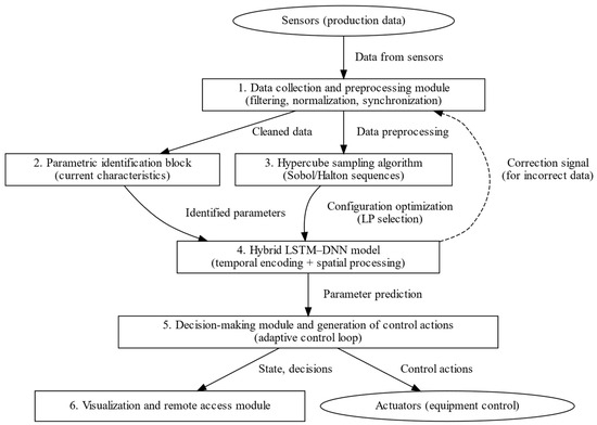
Figure 1.
Functional architecture of the intelligent information-control system (flowchart representation).
This approach creates a closed intelligent control loop with elements of self-learning and error correction. The hybrid LSTM–DNN model provides accurate forecasting, the hypercube probing algorithm enables efficient model tuning, and the validity module ensures data reliability [18]. As a result, the information and control system promptly adapts to process changes, increasing the efficiency and sustainability of metallurgical production [19].
Objects of metallurgical production, as a rule, are complex, multidimensional, dynamic systems with significant inertia, nonlinear behavior, and sensitivity to perturbations [20,21]. To describe them, we introduce the following:
- a state vector x(t) ∈ ℝn reflecting the internal process variables (e.g., temperatures in the furnace zones, impurity concentrations, filling levels, etc.);
- vector of controls u(t) ∈ ℝm, specifying the controlled influences (e.g., fuel supply, reagents, feed rate of raw materials); and
- vector of external disturbances w(t) ∈ ℝl (uncontrolled environmental influences, raw material properties, etc.).
- The measured output parameters of the process (controlled quantities) will be denoted as y(t) ∈ ℝp.
A system of nonlinear equations of state can give the dynamics of the object in the general case as follows:
where these are vector-functions specifying the laws of state change and outputs depending on the current state, control, and perturbing influences. These functions are derived from physical laws (mass and energy balances, reaction rate equations, etc.) or obtained by approximating experimental data [22]. Thus, in many units of metallurgy, the material balance equations are valid. For example, for a flow mixing unit, a linear conservative relationship can be written as follows:
where this represents the flow rate or mass of the j-th stream, and the coefficients reflect the stream topology and stoichiometric relations of the process. The presence of measurement errors leads to deviation of real data from ideal balances, which is accounted for by introducing perturbations and noise into the model. Nevertheless, the nominal mathematical model should satisfy the basic conservation laws of matter and energy and adequately reproduce the object’s dynamics [22,23].
Large time constants and lags characterize the temporal behavior of many metallurgical objects. For illustrative purposes, let us consider a simplified model of the thermal process. Let this value be the temperature of the metal in the furnace (state element), regulated by the supply of thermal energy (control). A first-order approximation can approximate the energy balance:
where C is the adequate heat capacity of the system, k is the heat loss coefficient, and is the ambient temperature. This differential equation describes the inertial growth of temperature under the action of heating with account of losses: at constant the temperature tends to a stationary value determined by the equality of heat input and dissipation. Such first-order lagged models are often used to describe the dynamics of metallurgical aggregates [24]. In general cases, however, the exact mathematical model of the control object can be very complex and multidimensional, and so in practice, identified black boxes based on machine learning methods are often used [25]. In particular, modern intelligent information and control systems increasingly usually include neural network simulators of technological objects, capable of reproducing the observed process dynamics and response to control actions [26,27]. Such a model makes it possible to analyze the impact of disturbances, predict the onset of critical equipment states, and optimize control in real time.
Note that the formalized object model includes stochastic components related to measurement noise and parameter uncertainty. These factors are taken into account when developing control methods and assessing system performance quality. In the present work, the mathematical model of the object is used in two ways:
- for data synthesis (generation of artificial scenarios, see below);
- when choosing the structure of the control model (in particular, the use of recurrent architectures to account for dynamics is justified).
2.1. Hybrid Neural Network Architecture LSTM-DNN
A hybrid neural network model combining a long short-term memory (LSTM) and a deep fully connected network (DNN) is chosen to solve the problems of prediction and adaptive control under complex dynamics. This approach is motivated by the limitations of individual architectures: classical full-link networks (DNNs) perform poorly on sequences over time because they lack a memory mechanism, and standard recurrent networks (RNNs) tend to “forget” long-term dependencies due to fading gradients. This assumption is consistent with recent studies on adaptive industrial data-driven systems and data reliability handling in industrial control applications [28,29]. The Long Short-Term Memory (LSTM) model is specifically designed to overcome these problems by introducing control input, output, and forgetting gates to preserve long-term information. However, recurrent memory alone is insufficient to fully reveal the nonlinear dependencies among many process variables. Adding a cascade of deep, fully connected layers, on the other hand, allows the model to generalize hidden patterns in the data and approximate complex nonlinear functions from features. Thus, the hybrid LSTM-DNN architecture combines the best of both worlds, leveraging temporal dependencies via LSTM and identifying static nonlinear relationships via DNN.
Logical structure of the model. Sequences of vectors of dimension n (consisting of n object parameters at each clock cycle of discrete time t) are fed to the input of the LSTM layer. The LSTM layer processes this input sequence of length T, storing information about previous observations in its internal state. Let us denote by the hidden state of LSTM at step t and by its memory element (cells). In the simplest case, one LSTM layer with k hidden neurons is used. Its operation is given by the following equations of vector form for each time step t (omitting matrix dimension indices):
where is the sigmoid, tanh is the hyperbolic tangent ;, is the vector of input, forgetting and output gates, respectively; is the candidate new memory values; , , -weighting matrices for the input vectors (including recurrent links to the previous hidden state; , , , , -thresholds (biases) of these neurons; the symbol denotes the element-by-element multiplication of the vectors. The initial state of the LSTM is usually initialized with a zero vector: = 0, = 0. As the sequence of inputs passes through, the recurrent network generates a sequence of hidden states , each containing rolled-up information about all previous steps. Thus, the last output has accumulated signs reflecting the dynamics of the process for the interval T.
Next, the DNN block comes into operation–several (one or more) fully connected layers of the neural network, processing the LSTM output and producing the target forecast. Let us denote by the compressed representation of the sequence (LSTM output at the last step). Then the output block may consist, for example, of two hidden layers with nonlinear activation and a final linear neuron to form a scalar forecast (if the task is regression of a single process indicator). Formally, this can be represented as follows:
where and are the weight matrix and displacement vector of the j-th DNN layer, is a nonlinear activation function on the layer (usually ReLU or similar). The vectors represent the activities of the hidden layer neurons. In this example, the final third layer produces a prediction without the activation function (i.e., linearly), which is suitable for continuous parameter prediction. If several parameters need to be predicted at once, the output vector is generated in a similar way (the dimensionality of is equal to the number of targets). All parameters of the network at the LSTM and DNN stages are selected during training on the data-usually by error back propagation with gradient optimization.
2.2. Component Targets and Model Properties
The considered architecture has a number of important properties that make it effective for metallurgical MIS tasks.
Firstly, the LSTM part serves to account for temporal dependencies: due to the presence of gates, it is able to store and retrieve information about long-term trends in the input signal without losing important correlations even with long sequences. This is especially significant for metallurgical processes where the current state depends on the prehistory (e.g., the quality of the produced alloy depends on the melting regime over the last hours, etc.).
Secondly, the DNN part acts as an approximator of complex nonlinearities: a multilayer fully connected network reveals hidden relationships between features and generates high-level generalized features. Thus, the hybrid model is able to simultaneously analyses dynamic patterns and nonlinear parameter relationships. It has been observed in the literature that such a combination yields higher accuracy and robustness compared to individual models. In particular, the LSTM-DNN model has demonstrated the ability to handle multivariate non-stationary time series and to correct measurements in real time [30]. In addition, the LSTM-DNN hybrid is experimentally shown to outperform both pure recurrent networks (e.g., GRU) and pure convolutional or full-link networks in terms of prediction accuracy and especially in terms of noise robustness-the ability to remain operational in the presence of noise and outliers in the data. High resistance to noise is achieved due to the fact that LSTM can filter short-term spikes and outliers in the signal at the expense of memory, and DNN detects average dependencies without reacting to small random fluctuations. The paper compares with alternative architectures (DNN, GRU, CNN, etc.), where the proposed hybrid showed the highest prediction accuracy with the lowest mean square deviation of the error and better stability when noise is added. Thus, the chosen architecture is justified both from a theoretical perspective (universal approximation and memory) and by empirical metrics of process modeling quality.
2.3. Algorithm for Probing the Hypercube with Low-Diversity Sequences
In order to efficiently tune the model and generate a variety of data scenarios, the hypercube probing method—scheduling experiments in parameter space using low-dispersed Sobol and Halton sequences—is used. The idea is to uniformly cover the multidimensional space of possible combinations of parameters affecting the system with a relatively small number of trial points [30]. In contrast to naive random search, quasi-random sequences (low-discrepancy sequences) fill the hypercube more uniformly, reducing “skips” and clustering of points. In fact, the Sobol and Halton sequences generate a deterministic sequence of coordinates in the d-dimensional unit cube , which has low dispersion (low discrepancy) relative to a uniform distribution. This means that for any sub-area , the relative number of sequence points in B approximates the volume of B much more accurately than for an equal number of points chosen independently at random. Quantitatively, the variance can be characterized by the stellar discrepancy metric , which for Sobol sequences is estimated as , i.e., it decreases much faster than for random sampling. Due to this, even with a limited number of trials, the quasi-random probing method covers the variant space almost uniformly.
Sobol and Halton sequences. Both are used to generate points in the hypercube, but are based on different principles. The Halton sequence is based on prime numbers: each dimension j corresponds to its own prime base (e.g., 2, 3, 5, 7, …). The n-th point of the sequence is obtained by representing the number n in a number system with base and “cutting off” the digits after the decimal point. For example, the coordinate in the first dimension is found as a fraction formed from the binary notation of the number n in reverse order (radical inversion in base 2). A similar process is performed for the second dimension with base 3, etc. Formally, the n-th point has the following coordinates:
where n = a0 + a1pj + a2pj +… is the decomposition of n in base , which is the so-called radical-inverted function (reflecting the digits after the decimal point). By using mutually simple bases, the Halton sequence generates non-trivial coverings of the unit cube. The Sobol sequence is constructed in a different way, and is based on binary fractions and primitive polynomials over GF(2). It is defined recurrently using the so-called guide vectors (numbers) chosen for each dimension. The generation uses a binary XOR operator and Gray code for index i, which ensures high uniformity when each next point is added. The Sobol algorithm is more complex to implement, but tabular values of the guide vectors for the desired dimension are usually available. In practice, the Sobol sequence often shows slightly more uniform coverage than Halton’s, especially in high dimensions, although it is sensitive to the proper choice of generation parameters [28]. Both approaches belong to quasi-random methods (pseudo-random vs. quasi-random): the sequence points are deterministic but mimic a uniformly random distribution when projected onto any subintervals.
Hypercube coverage and applications. Hypercube probing with low-dispersion points is applied in two key contexts:
- selection of model hyperparameters, and
- generation of synthetic data.
The hyperparameter search space for the hybrid LSTM–DNN model was explicitly defined prior to LD-based probing. The number of LSTM layers varied in the range of 1 to 3, with the number of hidden units per layer ranging from 32 to 128. The learning rate was selected within the interval [1 × 10⁻⁴, 1 × 10⁻²], and the batch size varied between 32 and 128 samples. Dropout regularization was applied with a coefficient in the range of 0 to 0.3. These bounds were normalized to the unit hypercube and sampled using Sobol or Halton sequences, after which inverse scaling was applied to obtain concrete hyperparameter configurations. The algorithm works as follows:
- Definition of the search space. The d hyperparameters are specified to set up the model. Each hyperparameter j is given a range or set of values that is normalized to the interval [0,1]. Thus, the space of all combinations is a unit d-dimensional cube .
- Generation of a quasi-random sample. We choose the sampling power N-the number of variants to be tried. Using a Sobol or Halton sequence generator we obtain a set of N points in . These points are distributed almost uniformly over the entire volume of space, which provides a variety of combinations.
- Reverse scaling of points. Each generated point is converted from a normalized representation to real hyperparameter values. This is performed by inverse linear scaling or by selecting the nearest acceptable discrete value for each parameter. The result is a specific set of hyperparameters .
- Quality assessment and selection of the best one. For each set , a hybrid LSTM-DNN model is trained (or tuned) and the quality is evaluated against a criterion (e.g., prediction error on the validation sample). Based on these results, an optimal combination of hyperparameters is selected . Studies show that initializing the search with a Sobol sequence often finds a better model and with less variability in the result than a random search. This is because uniform coverage does not allow us to “miss” narrow regions of the space with potentially good parameters. Related studies on anomaly detection and measurement validation in industrial sensor systems report comparable behavior under non-stationary operating conditions [31,32].
In this study, low-discrepancy hypercube probing is applied in two conceptually distinct but methodologically unified contexts: (i) hyperparameter optimization of the hybrid LSTM–DNN model, and (ii) generation and dataset-level integration of synthetic process scenarios with real data for dataset enrichment and robustness analysis.
In the second case, the same probing mechanism is used to enumerate object model scenarios and integrate the resulting synthetic trajectories with real production data. Here, the dimensions of the hypercube correspond to different experimental conditions, e.g., initial states , constant parameters of the object (raw material composition, inertia characteristics), and parameters of control actions (e.g., controller setpoint levels, signal variation profiles). The goal is to generate a set of artificial process trajectories covering the widest possible range of operating modes. The algorithm is similar:
- The range of each varying scenario variable is normalized (e.g., initial temperature-from the minimum to the maximum possible value, impurity concentration-within technical tolerance, etc.). The joint space of these variables forms a multidimensional rectangle (hypercube after scaling).
- Using the Sobol/Halton sequence, N points—a set of conditional scenarios—are selected. For example, one point may correspond to a combination: low temperature at the start, high concentration of impurity, average reagent flow rate, etc., while this is vice versa for another point, and so on, covering all corners of the space.
- For each such combination, a run of the mathematical model of the object described in Section 2 is carried out, either by simulation modeling of the process or by numerically solving the equations of dynamics. Synthetic time series —responses of the object to the given scenario conditions—are obtained.
- The generated data are included in the training set, supplementing the real data. Thus, a generalizable property is achieved, and the model is trained to recognize the behavior of the object in various situations, even those that are rarely encountered in the real observation history [33].
The hypercube probing algorithm has an important property of reproducibility. Since the Sobol and Halton sequences are deterministic, given a fixed sample size N and point rank, any researcher will achieve the same set of scenarios. This facilitates comparison and repetition of experiments by other experts. In addition, this algorithm is universal: by changing the generation function (e.g., by taking a Latin hypercube or another sequence with low variance), it is possible to adapt the coverage to specific requirements, such as the exclusion of boundary points or guaranteeing the absence of correlation between the selected parameters [34].
It is worth noting that low-discrepancy sequences have been shown to be effective in various neural network training settings. In particular, mini-sampling strategies or weight initialization based on Sobol sequences may accelerate convergence and improve the prediction accuracy of deep neural network models compared to random initialization. Thus, the hypercube probing method is embedded in our methodology not only at the data generation and hyperparameter selection stage, but also at stages related to the stability and optimization of the neural network model itself.
2.4. Dataset Construction and Synthesis
In order to train and verify the developed model, a representative dataset reflecting the variety of operating modes of a metallurgical facility is required [35]. In this work, the formation of the dataset was carried out in a combined way, using real production data and synthetically generated scenarios.
Actual data. The basic dataset is obtained from the real production automation system. The source is the archives of the automated control system of the copper smelting (beneficiation) process: readings of sensors and process parameter recorders collected in 24/7 mode. In particular, data was downloaded for the period from January to September 2024, including continuous daily measurements of approximately 30 key process parameters. These include reagent consumption, copper concentrate grade, flotation parameters, unit temperatures and pressures, and more. This multidimensional time sample reflects typical changes in process parameters during actual operation of the equipment. To use these data in the model, standard preprocessing was performed as follows: removal of coarse outliers and omissions, noise and noise filtering, and normalization of scales. Outlier removal was performed using a statistical three-sigma (3σ) rule applied to each parameter time series. Measurements deviating from the local mean by more than three standard deviations were classified as outliers and excluded prior to normalization. This preprocessing step reduced the influence of sporadic sensor spikes while preserving the overall dynamics of the process. Each parameter time series was scaled (e.g., by min-max or Z-score methods) to a comparable range so that no single feature dominates in order of magnitude. In addition, time synchronization was performed, and since measurements of different parameters may have been written at different frequencies, the data were brought to a single discrete step (e.g., min) by interpolation or averaging. The result is a reconciled data matrix:
where T is the number of time steps (observations), is the number of variables at each moment. To control overtraining, the dataset is divided into training, validation, and test: the model was trained on most of the sequences, and its predictive ability was tested on delayed time intervals not used in training. This approach provides an unbiased assessment of the generalizability of the model on new data.
Synthetic data. Despite the abundance of real data, there may be situations that are poorly represented in the archive records (e.g., emergency regimes, extreme values of concentrations, rare combinations of factors). In the context of this study, rare events are defined as infrequent but technologically significant process conditions that are weakly represented in historical datasets, including extreme or boundary values of technological parameters, emergency operating regimes, and abrupt disturbances that may adversely affect process stability and control performance. To increase the robustness of the model to such cases, the dataset was extended with artificially generated scenarios using the mathematical model of the object and the hypercube probing algorithm described above. Several critical factors were selected for variation: initial process conditions (e.g., initial melt temperature, initial impurity concentration), maximum and minimum values of control actions (intervals of reagent, air, and energy feed changes), and perturbation characteristics (possible abrupt changes in raw material composition, feed delays, etc.). Each factor is given a range covering both normal and extreme regimes. Furthermore, using the Sobol sequence in the space of these factors, different combinations (scenarios) are selected. For each scenario, the process was modeled on a computational simulator: the equations of the object dynamics were numerically solved when the corresponding control signals were applied and the specified perturbations were implemented. In this way, synthetic time series of parameters are obtained to complement the empirical set. It is important to emphasize that the synthetic data were added carefully so as not to disturb the statistical distribution: their share in the training sample was limited to approximately 20–30% to preserve the statistical characteristics of the real data distribution and to avoid bias toward synthetic scenarios; all generated samples were additionally checked for physical plausibility, including the absence of unrealistic values. This technique allowed us to significantly enrich the variability of training situations and improve the generalization ability of the model, especially in the prediction of rare events.
The proposed hybrid LSTM–DNN model was implemented using Python programming language (version 3.10) and the PyTorch deep learning framework (version 2.0). Model training and evaluation were performed on a workstation equipped with an NVIDIA RTX 3080 GPU (10 GB VRAM) (NVIDIA, Santa Clara, CA, USA), an Intel Core i9 CPU, and 64 GB of RAM (Intel Corporation, Santa Clara, CA, USA). GPU acceleration was used for neural network training, while data preprocessing and evaluation were executed on the CPU. This configuration ensured reproducible training and stable convergence of the model.
2.5. Noise Accounting and Noise Immunity
One of the goals of the methodology is to make the model highly robust to measurement noise and sensor failures [36,37]. To this end, noise immunity is laid down at several levels. Firstly, as noted, the LSTM-DNN architecture itself partially filters noise due to its properties. To evaluate noise robustness, additive zero-mean Gaussian noise was introduced into the test data. The noise variance was defined individually for each parameter type based on typical sensor accuracy: σ_T = 0.05T_nom for temperature, σ_P = 0.05P_nom for pressure, σ_L = 0.05L_nom for level, and σ_Q = 0.05Q_nom for flow rate, where the subscript “nom” denotes the nominal operating value. This corresponds to a 5% relative noise level, which is consistent with industrial sensor specifications. All noise components were independently generated and added to the corresponding signals. This metric allowed us to quantify how tolerant the model is to noise. In the experiments, the hybrid LSTM-DNN model showed a minimal increase in error when noise was added (only by ~8–9%), while for comparison the classical DNN showed an error increase of more than 20%, which confirms the high noise tolerance of the chosen approach.
The approach to the construction of the dataset and its enrichment with synthetic examples is aimed at ensuring scientific validity and reproducibility of the results. All stages of data collection and generation are documented and the datasets used (real and generated) can be re-acquired under the same initial conditions. Filtering and normalization of the data eliminates measurement artifacts, and the variety of scenarios (real and simulated) ensures that the model does not adjust only to a narrow range of situations, but works correctly over a wide range of process parameter variations. Such a carefully formed dataset serves as a reliable basis for training the hybrid model and its subsequent validation in conditions close to real conditions of metallurgical production [38].
The class diagram demonstrates the main components of the system (as logical modules/classes), their attributes (data), methods (functions), as well as connections and dependencies between them. The diagram is intended to describe the architecture of the ISU, which implements intelligent control of the metallurgical process based on temporal data, parametric identification, and optimization of the model configuration (Figure 2).
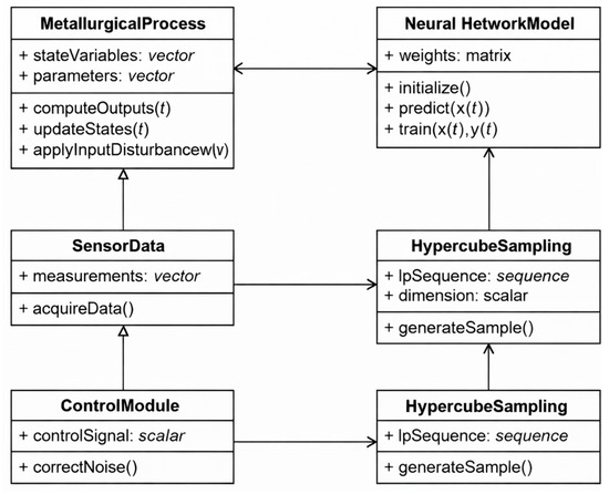
Figure 2.
UML class diagram of the intelligent information-control system.
The developed algorithm implements a combined approach to prediction and verification of technological parameters of metallurgical production.
Current measurements of process parameters , obtained from sensors (temperature, pressure, level, flow rate) are input into the system. Before being fed into the model, the data undergoes preliminary processing, including noise filtering, normalization, and formation of time windows.
To improve the stability and adaptability of the forecast, the LD-probing algorithm of the hypercube is used. At the probing stage, a uniform set of points in the space of input variables and hyperparameters is generated using low-dispersion Sobol or Halton sequences. The obtained points allow retraining of the hybrid neural network architecture LSTM-DNN by taking into account the current conditions of the technological process.
The updated model performs a prediction of the parameters , which is compared with the actual measurements. If the deviation modulus exceeds an acceptable threshold ε, an anomaly is recorded. If systematic anomalies are detected, a repeated cycle of LD-probing and model adaptation is started.
If unreliable values are present, they are corrected based on forecast or reconstruction methods on neighboring time points.
The final reliable value (initial or corrected) together with service marks is recorded in the information management system (IMS) for further use in process control and analytics.
Description of the operation of the anomaly detection and correction algorithm with LD-probing and hybrid LSTM-DNN model (Figure 3):
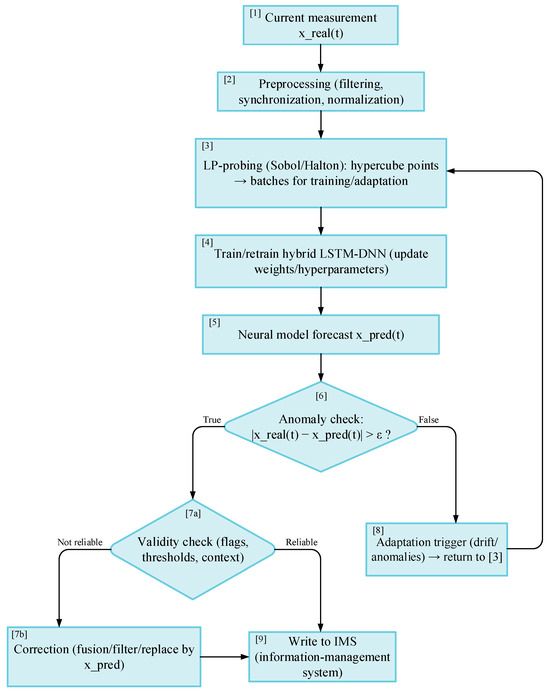
Figure 3.
Flowchart of the anomaly detection and correction algorithm.
- Input data acquisition: obtaining current measurements of process parameters (temperature, pressure, level, flow) from sensors and logging systems.
- Pre-processing: noise filtering, normalization, formation of time sequences for input to the model.
- LD-probing of the hypercube: generation of a set of points in the space of input variables and hyperparameters using low-dispersion Sobol or Halton sequences.
- Model adaptation: pretraining or tuning of the LSTM-DNN hybrid neural network architecture based on the sensing data. The procedure is performed periodically or when data drift/anomalies are detected.
- Prediction: using the updated LSTM-DNN model to obtain predicted values of process parameters.
- Anomaly detection: comparing the predicted value with the actual measurement; fixing the anomaly when the acceptable deviation threshold is exceeded.
- Validation: assessing the quality of the predicted or corrected value using an internal validity criterion.
- Correction: if unreliable values are detected, the correction is performed with reference to the model forecast or to the reconstructed value from neighboring time points.
- Recording in the IMS: fixing of the final reliable value in the information and control system together with service marks (time, source, status).
3. Results: Practical Realization of Technological Parameters Forecasting
The work uses a synthetic dataset generated on the basis of typical profiles of technological parameters (temperature, pressure, level, flow rate) in metallurgical systems. The objective is to demonstrate the concept and verify the stability of the prediction in the presence of noise, outliers, and anomalies.
Table 1 presents the results of a simulation experiment for temperature prediction of a metallurgical process facility using different neural network model architectures: hybrid LSTM-DNN, GRU, and CNN. Each row corresponds to a fixed moment of time with a step of 1 min on the interval from 0 to 20 min.

Table 1.
Experimental data (temperature).
For each time step, specific values are indicated as follows:
- real temperature value (T_real);
- predicted temperature value obtained from the LSTM-DNN (T_LSTM-DNN), GRU (T_GRU), and CNN (T_CNN) models;
- the calculated value of the failure function F(t), which determines the degree of deviation of the prediction from the real value; and
- binary indicator of reliability (1—the forecast is reliable, 0—deviation exceeds the threshold, the forecast is unreliable).
Table 1 shows the comparison of real and forecast temperatures (LSTM-DNN, GRU, CNN), rejection function, and reliability.
This form of presentation allows a comparative analysis of the models in terms of prediction accuracy, resistance to fluctuations, and adaptation ability when changing the technological mode. Based on the table, quality metrics (MAE, RMSE, R2) are calculated and a graphical comparison of curves of real and predicted values is formed (Table 2). To ensure stability of the reported metrics, a time-ordered train–validation–test split was applied. The model was trained on the first 70% of the time series, validated on the subsequent 15%, and tested on the final 15% of the data. This temporal separation prevents information leakage and confirms that the reported performance metrics are robust with respect to unseen operating regimes.
Table 2.
Quality metrics of temperature prediction.
Figure 4 shows the comparison of temperature predictions obtained using LSTM-DNN, GRU, and CNN models.
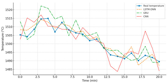
Figure 4.
Comparison of temperature predictions of different models.
Next, Table 3 of the experimental data: the real temperature values and predictions of the three models (LSTM, GRU, CNN) are presented for the time interval from 0 to 20 min. The failure function (if the error > 10 °C) and the confidence index (if the error ≤ 5 °C) for each model are also calculated.
Table 3.
Temperature forecast table.
To facilitate the analysis of temporal behavior, the data reported in Table 3 are further examined using time-series representations, as shown in Figure 5. Figure 5a depicts the temporal evolution of the actual temperature alongside the forecasts generated by the LSTM, GRU, and CNN models, enabling a direct comparison of model behavior over the entire observation horizon.
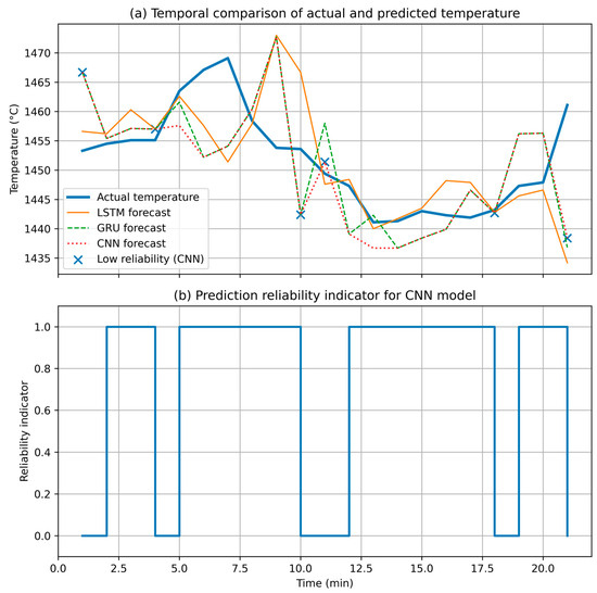
Figure 5.
Temporal dynamics of temperature forecasts and prediction reliability. Temporal comparison of actual temperature measurements and model-based forecasts obtained using LSTM, GRU, and CNN architectures, with time intervals of reduced prediction reliability highlighted (a), and the corresponding temporal evolution of the prediction reliability indicator for the CNN model (b).
The time-series analysis reveals that the LSTM- and GRU-based forecasts exhibit consistently stable dynamics and maintain close agreement with the measured temperature values throughout the considered time interval. In contrast, the CNN model displays several discrete temporal segments associated with reduced prediction reliability, which are explicitly highlighted by markers in Figure 5. These intervals coincide with locally increased deviations between the predicted and actual values, indicating reduced robustness of the CNN-based forecasts under certain dynamic conditions.
Figure 5b presents the temporal evolution of the prediction reliability indicator for the CNN model. The observed reliability degradation is localized in time and exhibits a clear correlation with forecast deviations, thereby confirming the diagnostic value of the proposed reliability assessment mechanism. This result demonstrates the suitability of the mechanism for continuous monitoring of model performance and for supporting data-driven decision-making in dynamic industrial environments.
Table 4 shows the simulated pressure data, the predictions from the LSTM, GRU, and CNN models, and the confidence score of each prediction.
Table 4.
Comparison of simulated pressure data with predictions from LSTM, GRU, and CNN models, including confidence scores.
A similar time-series–based analysis was performed for another key process variable, namely pressure, in order to verify the consistency and generality of the proposed approach across different types of measured parameters.
To further analyze the temporal behavior of the pressure data reported in Table 4, the results are additionally represented in the form of time-series plots, as shown in Figure 6. Figure 6a illustrates the temporal evolution of the actual pressure and the corresponding forecasts generated by the LSTM, GRU, and CNN models.
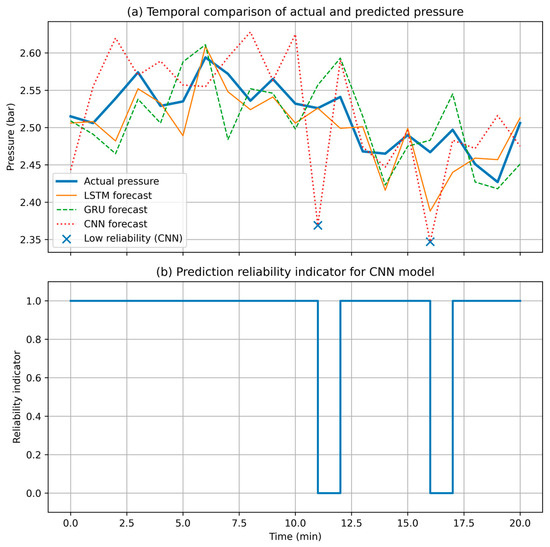
Figure 6.
Temporal dynamics of pressure forecasts and prediction reliability. Temporal comparison of actual pressure measurements and model-based forecasts obtained using LSTM, GRU, and CNN architectures, with time intervals of reduced prediction reliability highlighted (a) and the corresponding temporal evolution of the prediction reliability indicator for the CNN model (b).
The analysis shows that the LSTM- and GRU-based forecasts remain stable and closely follow the actual pressure values over the entire observation interval. In contrast, the CNN model exhibits isolated time instants characterized by reduced prediction reliability, which are explicitly marked in the figure.
Figure 6b presents the temporal evolution of the prediction reliability indicator for the CNN model. The observed reliability degradation is localized in time and correlates with increased deviations between the predicted and actual pressure values, further confirming the diagnostic capability of the proposed reliability assessment mechanism.
Figure 7 summarizes the pressure changes over time, showing the comparison between the real values and the LSTM-DNN model prediction.
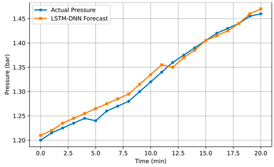
Figure 7.
Pressure: Real values and model prediction.
Level change (L) over time shows the real behavior and prediction of the LSTM-DNN model (Figure 8). Flow rate variation (Q) similarly compares measured and predicted values (Figure 9).
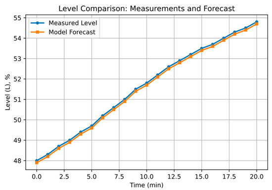
Figure 8.
Level: Real value and prediction of the model.
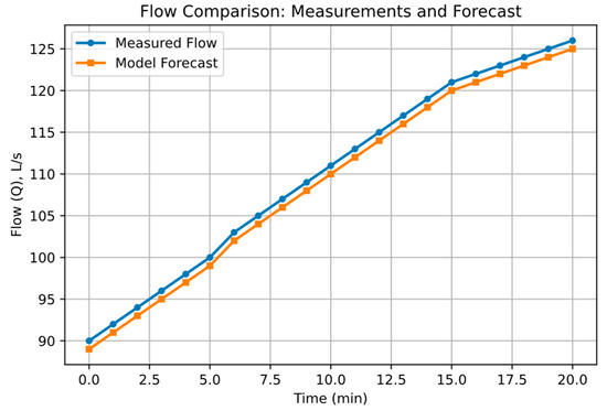
Figure 9.
Flow rate: Real value and model prediction.
Figure 10 shows the failure function constructed from four metallurgical process parameters: temperature, pressure, level, and flow rate.
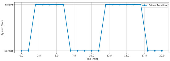
Figure 10.
Process-based failure function.
If at any time at least one parameter is out of the acceptable range, the system is considered to be in a failure state (value 1). Otherwise, it is considered to be in a normal state (value 0). Such peaks on the graph signal potential violations of the technological mode.
Table 5 contains synthetic (modeled) data on parameter values at each moment of time (in 1 min increments). Parameters are presented as follows:
Table 5.
Synthetic time-series dataset for multiparameter forecasting and reliability evaluation.
- real value;
- forecast of the neural network model (LSTM-DNN);
- absolute forecast error (modulo); and
- a binary label of the forecast reliability (true/false) by the threshold value of the error.
Table 5 allows the evaluation of forecast accuracy, identifying failures, visualizing anomalies, and demonstrating the effectiveness of the control architecture used.
The above characteristics (Figure 9) illustrate the behavior of four key parameters of the technological process of metallurgical production [39] in the time interval from 0 to 20 min:
- temperature shows a steady increase, which is typical of the material-heating stage;
- pressure increases more linearly, reflecting the increasing process load;
- the level fluctuates, indicating possible feed and discharge cycles; and
- the flow rate shows step dynamics corresponding to pumping equipment operating modes (Figure 11).
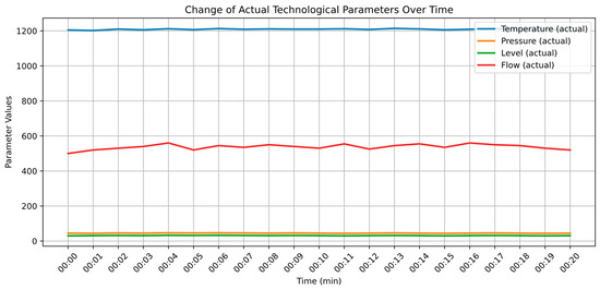 Figure 11. Change in actual technological parameters over time.
The following is a description of the mechanism of correction of anomalous values based on the neural network model prediction [40].
The model of measurement correction is applied via neural network model prediction. The mechanism of automatic correction of anomalous values resulting from noise, sensor failures, or external disturbances is provided within the framework of building a reliable information and control system. The correction is based on the comparison of the current measured value, with the prediction obtained from the hybrid neural network model LSTM-DNN [41,42].
Let denote the measured value of the technological parameter at time t, and denote the corresponding predicted value obtained from the model. A threshold of acceptable deviation ε is introduced, and is determined either on the basis of statistical analysis or according to the technical regulations of the process [43,44,45].
The correction is carried out according to the following principle:
- if the deviation does not exceed the threshold ε, the value is recognized as valid and stored, and
- if the deviation exceeds the threshold, the value is considered anomalous and is replaced by the model prediction:
This approach allows the exclusion of unreliable measurements from the subsequent control or analysis loop, ensuring the resilience of the system to emissions and localized disturbances.
The anomaly detection threshold ε was defined separately for each technological parameter based on industrial tolerances. Specifically, ε_T = 5 °C for temperature, ε_P = 0.2 bar for pressure, ε_L = 3% of nominal level for material level, and ε_Q = 5% of nominal value for flow rate. These thresholds reflect acceptable deviations in metallurgical operation and were used uniformly across all experiments (Algorithm 1).
| Algorithm 1 Anomaly Detection and Correction Using LSTM–DNN Forecast |
| Input: x_real(t) –measured value of the process parameter at time t x_pred(t) –predicted value obtained from the LSTM–DNN model ε –anomaly detection threshold context– –additional process context and recent history Output: x_out(t) –reliable value written to the information-control system 1: Compute deviation: Δ(t) = |x_real(t) − x_pred(t)| 2: if Δ(t) ≤ ε then 3: x_out(t) ← x_real(t) 4: Write x_out(t) to the information-control system 5: else 6: Compute corrected value: x_corr(t) = C(x_real(t), x_pred(t), context) 7: Perform admissibility and consistency check for x_corr(t) 8: if admissibility conditions are satisfied then 9: x_out(t) ← x_corr(t) 10: Write x_out(t) to the information-control system 11: else 12: Generate operator alert 13: Activate backup data sources or trigger re-identification 14: end if 15: end if |
Pseudocode of the anomaly detection and correction algorithm:
- Input: current measurement and model forecast for the same point in time.
- Anomaly test: if the absolute error exceeds the threshold ε-consider the measurement suspicious.
- Correction : operator C is the chosen method (median/exponential filter, model-base interpolation, recalculation by T-P-Q-L links, or mixing
- Anomaly free validity: additional consistency rules (gradients, physical constraints, flux balance).
- Output: either the original , or the adjusted goes to the IMS when the criteria are not met-alarm and switch to redundant sensors/repeat identification.
Figure 12 shows the time series of the technological process parameter with a sampling step of 1 min.
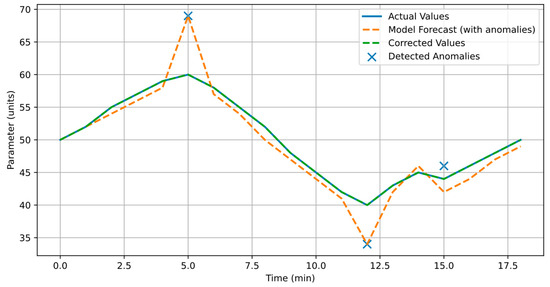
Figure 12.
Detection and correction of process parameter anomalies.
- Blue line: true values of the parameter, reflecting the normal behavior of the system.
- Red line: forecast of hybrid neural network model LSTM-DNN, distorted by introduced anomalies modeling failures in measurement channels (spikes, outliers, drift).
- Green line: values after processing by the correction module, with anomalies removed or compensated for based on comparison with the model prediction and LD-probing of the hypercube for adaptation.
At the intervals where the system detected anomalies, the forecast was subjected to correction, which allowed the data to be restored to a level close to the true values. This approach increases the reliability of measurement information and reduces the risk of erroneous control actions in the IMS.
Methodology for correction of anomalies in process parameters: The process of anomaly correction is based on the joint use of hybrid neural network architecture LSTM-DNN and hypercube probing algorithm with low-dispersed sequences (Sobol/Halton) to improve the stability and accuracy of prediction.
- Data acquisition and preparation: Raw parameter values (temperature, pressure, level, flow rate) are acquired from sensors in real time. Coarse outliers are filtered and data normalization is performed at this stage.
- LSTM-DNN model-based prediction: A trained model capable of accounting for both short-term fluctuations and long-term parameter dependencies is used to predict current and future values.
- Built-in LD hypercube probing: Periodically or when data drift is detected, the generation of test scenarios (hypercube of input conditions) is triggered using low-dispersion sequences. The resulting points are used to refine the model to ensure adaptation to changing process conditions.
- Anomaly detection: Comparison of actual measurements with the model prediction. Anomalies are defined as values that are outside the defined deviation thresholds.
- Value Correction: If an anomaly is detected, the value is replaced with a corrected value based on the predicted model and the nearest valid measurements, taking into account the physical relationships between the parameters.
- Record in the MIS: The corrected (or confirmed as valid) value is entered into the control system, along with the validity labels, type of correction, and algorithm performance statistics.
4. Discussion
This approach makes it possible not only to promptly eliminate one-time failures, but also to adapt to changes in the operating mode of the equipment, while maintaining high reliability of measurement data.
Larger prediction deviations observed for certain parameters can be attributed to their higher inertia and delayed response to control actions, particularly for temperature and level dynamics. In contrast, pressure and flow rate exhibit faster dynamics and stronger direct coupling with control inputs, resulting in lower prediction uncertainty. These differences are consistent with the physical characteristics of metallurgical processes and confirm that prediction difficulty is parameter dependent.
The considered architecture of the information and control system (Figure 1), including the hybrid neural network model LSTM-DNN and the hypercube probing module with low-dispersed sequences (Sobol, Halton), demonstrated improved quality indicators for predicting the parameters of the technological process of metallurgical production.
Comparative modeling results (Table 2) showed that the proposed architecture provides a 7–15% reduction in the average values of MAE, RMSE metrics and an increase in the determination coefficient R2 by 7–15% when compared to the basic LSTM, GRU, and CNN models. The application of LD sequences at the stage of model adaptation allowed for a more uniform coverage of the space of input conditions and hyperparameters compared to the Monte Carlo method, which had a positive effect on the stability and generalization ability of the neural network model.
A comparative analysis of approaches to adaptation of neural network models showed that the use of LD-probing (Sobol, Halton sequences) has a fundamental advantage over random point selection by the Monte Carlo method. In the case of Monte Carlo, the sample of hyperparameters and input conditions is unevenly distributed, which, with a limited number of iterations, leads to incomplete coverage of areas with critical technological modes. LD sequences, on the contrary, provide quasi-regular coverage of the hypercube of parameters, which increases the probability of hitting the areas where the model accuracy degrades. This is particularly important in metallurgical production, where unlikely but technologically significant regimes (e.g., overheating of metal, critical pressure, or flow rate spikes) can lead to accidents.
The algorithm of anomaly detection and correction (Figure 3) allowed us to reduce the share of unreliable measurements to less than 2% of the total data (against 8–12% in control experiments without correction). Parameter values deviating from the model prediction by more than the threshold value ε (formula 8) were automatically classified as anomalous and corrected according to the agreed rule:
The visualization results (Figure 4, Figure 5, Figure 6, Figure 7, Figure 8, Figure 9 and Figure 10) confirm that the proposed mechanism efficiently recovers correct values of temperature, pressure, level, and flow rate even with sudden data spikes caused by noise, sensor drift, or simulated failures.
The combined operation of LD sensing and the hybrid LSTM-DNN architecture not only improves prediction accuracy at steady-state sections of the process, but also maintains stability in the event of abrupt changes in process conditions. The LSTM component provides consideration of time dynamics and dependence between parameters, and the DNN component provides nonlinear representation of multidimensional dependencies between the system state and control actions. The result is a more stable model that is less susceptible to retraining and capable of rapid recovery of accuracy after sensor drift or changes in the composition of the initial data.
In general, the integration of the prediction module based on the hybrid architecture LSTM-DNN with the LD-probing procedure and the mechanism of adaptive correction of anomalies provides an increase in the reliability of measurement information, which is critical for the stable operation of the IMS in conditions of high variability of technological modes.
5. Conclusions
The integrated methodology of forecasting and monitoring of technological parameters of metallurgical production based on hybrid architecture LSTM-DNN and hypercube probing algorithm using low-disperse sequences (Sobol, Halton) is proposed.
An anomaly module has been developed that provides automatic detection and correction of unreliable temperature, pressure, level, and flow measurements in real time. The module is integrated into the information and control system, which allowed an increase in the stability of control processes. Experimental results have shown that the application of LD-probing in model pretraining allows for a reduction in the adaptation time and improvements in the prediction accuracy compared to the initial model without probing procedure.
The hybrid LSTM-DNN architecture proved effective under highly correlated parameters and system lags, providing a coefficient of determination R2 above 0.92 for predicting key process parameters in the test environment. A comparative analysis with alternative architectures (GRU and CNN) demonstrated the advantage of the proposed approach in terms of MAE, RMSE, and R2 metrics, which confirms its effectiveness for industrial automation tasks.
A limitation of the proposed approach is the assumption of continuous and sufficiently dense sensor data streams; application to systems with sparse measurements or fundamentally different metallurgical units may require additional retraining and parameter adjustment.
This study proposes an integrated methodology for forecasting and monitoring technological parameters of metallurgical production based on a hybrid LSTM–DNN architecture and a hypercube probing algorithm using low-discrepancy sequences (Sobol and Halton).
Despite the demonstrated effectiveness of the proposed hybrid LSTM–DNN architecture, several limitations should be noted. The current study assumes the availability of continuous and sufficiently dense sensor data streams, as well as a stable process configuration within a single industrial domain. Moreover, prediction uncertainty is not explicitly quantified, and the reliability assessment relies on a deterministic threshold-based mechanism, which may be insufficient under strongly time-varying operating conditions or abrupt regime transitions.
Future research will focus on extending the proposed framework toward uncertainty-aware forecasting and reliability assessment, including probabilistic or distribution-based prediction models. Another promising direction involves incorporating adaptive uncertainty quantification and dynamic thresholding mechanisms to enhance robustness under severe non-stationarity. In addition, the integration of the proposed approach with cross-domain or federated learning paradigms will be investigated to improve generalization while preserving real-time applicability in industrial information-control systems.
The proposed methodology is applicable to a wide range of metallurgical and related industries, where the accuracy of prediction and reliability of control of process parameters are critical. Implementation of the system leads to a reduced risk of emergency situations, increases energy efficiency of processes, and optimizes equipment maintenance schedules due to early detection of anomalies and data drift.
Author Contributions
Conceptualization, J.S. and B.T.; methodology, J.S., B.T. and U.M.; software, J.S. and U.M.; validation, J.S., G.B. and U.M.; formal analysis, G.B. and B.B.; investigation, J.S. and U.M.; resources, B.T. and G.B.; data curation, U.M. and G.B.; writing—original draft preparation, J.S. and U.M.; writing—review and editing, B.T., G.B. and B.B.; visualization, U.M.; supervision, B.T.; project administration, B.T.; funding acquisition, B.B. All authors have read and agreed to the published version of the manuscript.
Funding
This research received no external funding.
Data Availability Statement
All used datasets are available online, and are openly accessible.
Conflicts of Interest
The authors declare no conflicts of interest.
Abbreviations
The following abbreviations are used in this manuscript:
| ICS | Information and control systems |
| PID | Proportional–Integral–Derivative Controller |
| IIoT | Industrial Internet of Things |
| LSTM-DNN | Long Short-Term Memory networks and Deep Neural Networks |
| APCS | Automated process control system |
| SCADA | Supervisory Control and Data Acquisition |
| LIMS | Laboratory Information Management System |
| MES | Manufacturing Execution System |
| ERP | Enterprise Resource Planning |
| FC | Fully Connected |
| LD | Low-Discrepancy Sequences |
| IICS | Intelligent Information and Control Systems |
| ML | Machine Learning |
| AI | Artificial Intelligence |
References
- Sun, H. Optimizing Manufacturing Scheduling with Genetic Algorithm and LSTM Neural Networks. Int. J. Simul. Model. 2023, 22, 508–519. [Google Scholar] [CrossRef]
- Essien, A.E.; Giannetti, C. A Deep Learning Model for Smart Manufacturing Using Convolutional LSTM Neural Network Autoencoders. IEEE Trans. Ind. Informatics 2020, 16, 6069–6078. [Google Scholar] [CrossRef]
- Hieu, N.T.; di Francesco, M.; Yla-Jaaski, A. A multi-resource selection scheme for virtual machine consolidation in cloud data centers. In Proceedings of the International Conference on Cloud Computing Technology and Science, CloudCom, Vancouver, BC, Canada, 30 November–3 December 2015. [Google Scholar] [CrossRef]
- Rayan, A.; Nah, Y. Resource prediction for big data processing in a cloud data center: A machine learning approach. IEIE Trans. Smart Process. Comput. 2018, 7, 478–488. [Google Scholar] [CrossRef]
- Avazov, K.; Sevinov, J.; Temerbekova, B.; Bekimbetova, G.; Mamanazarov, U.; Abdusalomov, A.; Cho, Y.I. Hybrid Cloud-Based Information and Control System Using LSTM-DNN Neural Networks for Optimization of Metallurgical Production. Processes 2025, 13, 2237. [Google Scholar] [CrossRef]
- Zhang, R.; Cao, S. Extending reliability of mmwave radar tracking and detection via fusion with camera. IEEE Access 2019, 7, 137047–137061. [Google Scholar] [CrossRef]
- Hochreiter, S.; Schmidhuber, J. Long short-term memory. Neural Comput. 1997, 9, 1735–1780. [Google Scholar] [CrossRef]
- Hewamalage, H.; Bergmeir, C.; Bandara, K. Recurrent neural networks for time series forecasting: Current status and future directions. Int. J. Forecast. 2021, 37, 388–427. [Google Scholar] [CrossRef]
- Wen, L.; Li, X.; Gao, L.; Zhang, Y. A new convolutional neural network-based data-driven fault diagnosis method. IEEE Trans. Ind. Electron. 2018, 65, 5990–5998. [Google Scholar] [CrossRef]
- Qian, Q.; Zhang, B.; Li, C.; Mao, Y.; Qin, Y. Federated transfer learning for machinery fault diagnosis: A comprehensive review of technique and application. Mech. Syst. Signal Process. 2025, 223, 111837. [Google Scholar] [CrossRef]
- Zhou, J.; Qin, Y.; Chen, D.; Liu, F.; Qian, Q. Remaining useful life prediction of rolling bearings using a reinforced memory GRU network. Adv. Eng. Inform. 2022, 53, 101682. [Google Scholar] [CrossRef]
- Wang, Z.; Chen, Z.; Li, C. Integrated dispersion manifold distance: A new distribution discrepancy metric for fault diagnosis under time-varying conditions. Reliab. Eng. Syst. Saf. 2022, 223, 108468. [Google Scholar]
- Temerbekova, B.M. Application of Systematic Error Detection Method to Integral Parameter Measurements in Sophisticated Production Processes and Operations. Tsvetnye Met. 2022, 2022, 79–86. [Google Scholar] [CrossRef]
- Liu, C.; Tang, D.; Zhu, H.; Nie, Q. A novel predictive maintenance method based on deep adversarial learning in the intelligent manufacturing system. IEEE Access 2021, 9, 49557–49575. [Google Scholar] [CrossRef]
- Turgunboev, A.Y.; Temerbekova, B.M.; Usmanova, K.A.; Mamanazarov, U.B. Application of the microwave method for measuring the moisture content of bulk materials in complex metallurgical processes. Chernye Met. 2023, 2023, 23–28. [Google Scholar] [CrossRef]
- Banitalebi-Dehkordi, A.; Vedula, N.; Pei, J.; Xia, F.; Wang, L.; Zhang, Y. Auto-Split: A General Framework of Collaborative Edge-Cloud AI. In Proceedings of the ACM SIGKDD International Conference on Knowledge Discovery and Data Mining, Online, 14–18 August 2021. [Google Scholar] [CrossRef]
- Rahman, M.A.; Shakur, S.; Ahamed, S.; Hasan, S.; Rashid, A.A.; Islam, A.; Haque, S.S.; Ahmed, A. A Cloud-Based Cyber-Physical System with Industry 4.0: Remote and Digitized Additive Manufacturing. Automation 2022, 3, 400–425. [Google Scholar] [CrossRef]
- Zhang, X.; Cao, Z.; Dong, W. Overview of Edge Computing in the Agricultural Internet of Things: Key Technologies, Applications, Challenges. IEEE Access 2020, 8, 141748–141761. [Google Scholar] [CrossRef]
- Igamberdiyev, H.Z.; Yusupbekov, A.N.; Zaripov, O.O.; Sevinov, J.U. Algorithms of adaptive identification of uncertain operated objects in dynamical models. Procedia Comput. Sci. 2017, 120, 854–861. [Google Scholar] [CrossRef]
- Rai, R.; Tiwari, M.K.; Ivanov, D.; Dolgui, A. Machine learning in manufacturing and industry 4.0 applications. Int. J. Prod. Res. 2021, 59, 4773–4778. [Google Scholar] [CrossRef]
- Shilpashree, S.; Patil, R.R.; Parvathi, C. Cloud computing an overview. Int. J. Eng. Technol. 2018, 7, 2743–2746. [Google Scholar] [CrossRef]
- Li, Z.; Zhao, H.; Shi, J.; Huang, Y.; Xiong, J. An Intelligent Fuzzing Data Generation Method Based on Deep Adversarial Learning. IEEE Access 2019, 7, 49327–49340. [Google Scholar] [CrossRef]
- Stadtfeld, H.J. Industry 4.0 and its implication to gear manufacturing. In Proceedings of the American Gear Manufacturers Association Fall Technical Meeting 2015, AGMA FTM 2015, Detroit, MI, USA, 18–20 October 2015. [Google Scholar]
- Anagnostis, A.; Papageorgiou, E.; Bochtis, D. Application of artificial neural networks for natural gas consumption forecasting. Sustainability 2020, 12, 6409. [Google Scholar] [CrossRef]
- Temerbekova, B.M.; Mamanazarov, U.B.; Bekimbetov, B.M.; Ibragimov, Z.M. Development of integrated digital twins of control systems for ensuring the reliability of information and measurement signals based on cloud technologies and artificial intelligence. Chernye Met. 2023, 2023, 39–46. [Google Scholar] [CrossRef]
- Cinar, E.; Kalay, S.; Saricicek, I. A Predictive Maintenance System Design and Implementation for Intelligent Manufacturing. Machines 2022, 10, 1006. [Google Scholar] [CrossRef]
- Dinata, R.K.; Retno, S.; Hasdyna, N. Minimization of the Number of Iterations in K-Medoids Clustering with Purity Algorithm. Rev. D’intelligence Artif. 2021, 35, 193–199. [Google Scholar] [CrossRef]
- Wang, Z.; Chang, J.; Ju, Q.-P.; Xie, F.-M.; Wang, B.; Li, H.-W.; Wang, B.; Lu, X.-C.; Fu, G.-Q.; Liu, Q. Prediction model of end-point manganese content for BOF steelmaking process. ISIJ Int. 2012, 52, 1585–1590. [Google Scholar] [CrossRef]
- Liu, C.; Tang, L.; Liu, J. A Stacked Autoencoder with Sparse Bayesian Regression for End-Point Prediction Problems in Steelmaking Process. IEEE Trans. Autom. Sci. Eng. 2020, 17, 550–561. [Google Scholar] [CrossRef]
- Qiu, K.; Li, J.; Chen, D. Optimized long short-term memory (LSTM) network for performance prediction in unconventional reservoirs. Energy Rep. 2022, 8, 15436–15445. [Google Scholar] [CrossRef]
- Zarzycki, K.; Ławryńczuk, M. Advanced predictive control for GRU and LSTM networks. Inf. Sci. 2022, 616, 229–254. [Google Scholar] [CrossRef]
- Tao, F.; Qi, Q.; Wang, L.; Nee, A.Y.C. Digital Twins and Cyber–Physical Systems toward Smart Manufacturing and Industry 4.0: Correlation and Comparison. Engineering 2019, 5, 653–661. [Google Scholar] [CrossRef]
- Lee, J.; Bagheri, B.; Kao, H.-A. A cyber–physical systems architecture for Industry 4.0-based manufacturing systems. Manuf. Lett. 2015, 3, 18–23. [Google Scholar] [CrossRef]
- Chandola, V.; Banerjee, A.; Kumar, V. Anomaly detection: A survey. ACM Comput. Surv. 2009, 41, 18–23. [Google Scholar] [CrossRef]
- Zonta, T.; da Costa, C.A.; da Rosa Righi, R.; de Lima, M.J.; da Trindade, E.S.; Li, G.P. Predictive maintenance in the Industry 4.0: A systematic literature review. Comput. Ind. Eng. 2020, 150, 106889. [Google Scholar] [CrossRef]
- Li, S.; Xu, B.; Chung, T.L. Definition extraction with LSTM recurrent neural networks. In Chinese Computational Linguistics and Natural Language Processing Based on Naturally Annotated Big Data: 15th China National Conference, CCL 2016, and 4th International Symposium, NLP-NABD 2016, Yantai, China, 15–16 October 2016, Proceedings; Lecture Notes in Computer Science; Including Subseries Lecture Notes in Artificial Intelligence and Lecture Notes in Bioinformatics; Springer: Berlin/Heidelberg, Germany, 2016. [Google Scholar] [CrossRef]
- Cortez, B.; Carrera, B.; Kim, Y.J.; Jung, J.Y. An architecture for emergency event prediction using LSTM recurrent neural networks. Expert Syst. Appl. 2018, 97, 315–324. [Google Scholar] [CrossRef]
- Nosouhian, S.; Nosouhian, F.; Khoshouei, A.K. A review of recurrent neural network architecture for sequence learning: Comparison between LSTM and GRU. Preprints 2021. [Google Scholar] [CrossRef]
- Pudikov, A.; Brovko, A. Comparison of LSTM and GRU Recurrent Neural Network Architectures. In Studies in Systems, Decision and Control; Springer: Berlin/Heidelberg, Germany, 2021; Volume 337. [Google Scholar] [CrossRef]
- Jiang, Z.; Yuan, S.; Ma, J.; Wang, Q. The evolution of production scheduling from Industry 3.0 through Industry 4.0. Int. J. Prod. Res. 2022, 60, 3534–3554. [Google Scholar] [CrossRef]
- Kumas, E.; Erol, S. Digital Twins as Key Technology in Industry 4.0. J. Polytech. Politek. Derg. 2021, 24, 691–701. [Google Scholar]
- Gulyamov, S.; Temerbekova, B.; Mamanazarov, U. Noise Immunity Criterion for the Development of a Complex Automated Technological Process. E3S Web Conf. 2023, 452, 3014. [Google Scholar] [CrossRef]
- Zhen, T.; Yan, L.; Yuan, P. Walking gait phase detection based on acceleration signals using LSTM-DNN algorithm. Algorithms 2019, 12, 253. [Google Scholar] [CrossRef]
- Piel, É.; Marquet, P.; Soula, J.; Dekeyser, J.L. Real-time systems for multi-processor architectures. In Proceedings of the 20th International Parallel and Distributed Processing Symposium, IPDPS 2006, Rhodes Island, Greece, 25–29 April 2006. [Google Scholar] [CrossRef]
- Cao, K.; Zhang, T.; Huang, J. Advanced hybrid LSTM-transformer architecture for real-time multi-task prediction in engineering systems. Sci. Rep. 2024, 14, 4890. [Google Scholar] [CrossRef] [PubMed]
Disclaimer/Publisher’s Note: The statements, opinions and data contained in all publications are solely those of the individual author(s) and contributor(s) and not of MDPI and/or the editor(s). MDPI and/or the editor(s) disclaim responsibility for any injury to people or property resulting from any ideas, methods, instructions or products referred to in the content. |
© 2026 by the authors. Licensee MDPI, Basel, Switzerland. This article is an open access article distributed under the terms and conditions of the Creative Commons Attribution (CC BY) license.