Finite-Time Prescribed Performance Tracking Control for Unmanned Helicopter System Using Neural Network

Abstract

In this paper, a composite finite-time prescribed performance tracking control scheme is presented for an unmanned helicopter (UH) system subject to performance constraints, model uncertainties and external perturbations. A new finite-time neural network disturbance observer (FTNNDO) with adaptive laws is designed to deal with the external disturbances and model uncertainties, which not only accelerate the convergence rate in finite time but also eliminate the complicated differential calculation in the traditional backstepping scheme. Using the continuous adaptive law, the neural network (NN) approximate errors can be effectively estimated and compensated online without the chattering and gain overestimation caused by traditional methods, thus further enhancing the robustness of the system. To constrain the tracking performance of the transient process and steady-state accuracy, a novel prescribed performance function is designed to preset the tracking errors within prescribed boundaries. Based on the FTNNDO and barrier Lyapunov function (BLF), an improved finite-time tracking controller is designed to achieve fast convergence with prescribed performance. By using Lyapunov synthesis, it is strictly proven that the finite-time convergence of the closed-loop control system can be achieved and tracking errors are always within the prescribed performance bounds. In the end, simulation results for the UH tracking control system are given to demonstrate the effectiveness of developed control scheme.

1. Introduction

Over the past few decades, unmanned helicopters have been paid much considerable attention and received extensive research owing to their diverse and flexible flight capabilities. However, it remains challenging to design an effective, robust and high-precision tracking controller for UHs due to their properties of nonlinearities, uncertainties, coupling dynamics and sensitivities to external disturbances. To cope with these impacts and further improve the performance of the tracking controller, various controller design techniques were developed and applied in actual unmanned helicopter systems, to name a few, model predictive control, H∞, backstepping control, sliding mode control, intelligent control and adaptive control methods, etc. [1,2,3,4,5,6].

Nowadays, modern flight tasks require UH achieving control objectives within a specified time. Different from asymptotic control methods, a finite-time control strategy can achieve a faster response rate, higher control accuracy and more excellent anti-disturbance ability [7,8], which is more suitable for the situation that requires high control performance. Distinctly, it is of great significance to develop a finite-time convergence control scheme for UHs. So far, many control methods that can achieve finite-time convergence have been developed [9,10,11,12]. Among these techniques, backstepping is one of the most effective control methods to handle the tracking control problems of UHs [13,14]. Based on this framework, the filter-based dynamic surface control (DSC) [15] and modified command-filtered backstepping control (CFBC) [16] approaches were proposed; however, the control laws designed using these methods can only achieve asymptotic stability. A modified CFBC approach was presented and able to achieve finite-time convergence under the backstepping framework by using robust differentiators, compensated virtual control signals and novel error compensation mechanisms [17]. Note that the effects of unknown system uncertainties and external disturbances have not been considered in [17], the filter and compensator are still additionally designed to deal with the differential value and filtering error at each step in backstepping procedure, which increases the computational complexity of design. Therefore, the above methods still have a certain degree of conservatism and can be further modified.

Moreover, UH needs to perform higher quality flight missions to ensure not only the good steady-state characteristics but also the good transient characteristics [18]. These characteristics of outputs such as overshoot and adjustment time, need to be constrained to achieve smooth and fast tracking performance [19]. Since the BLF is convenient to handle the constraint control problem, many robust constraint controllers are designed to realize the restricted tracking in combination with the BLF and other adaptive control schemes [20,21,22]; however, these methods mainly focused on the steady-state error or state amplitude constraints and paid less attention to the transient performance constraints. A meaningful concept called prescribed performance was introduced in [23], where the constraints on the steady-state tracking error, maximum overshoot and convergence rate can be tackled simultaneously, but the inverse function of this method may cause complex computing problems [24,25,26]. Besides, these prescribed performance methods all depend on the initial system state, of which the sign and value must be known in advance, causing inconvenience in practical applications. In this article, a new prescribed performance strategy is designed, which can adjust the initial boundary adaptively and avoid the influence of the initial value during design.

It is well known that UH is a complex and unstable high-order nonlinear system, where the external disturbances and uncertainties will degrade the tracking performance and reduce the robustness of the system. In order to enhance the closed-loop control performance and anti-interference ability of the system, neural network and nonlinear disturbance observer (NDO) have been widely studied and applied in UH systems [27,28,29,30]. In [31], many disturbance-observer-based control (DOBC) schemes have been summarized, and the industrial applications of those methods were researched and reviewed. In [28], NNs were applied to approximate unknown uncertainties, and an NDO was simultaneously designed to deal with unknown but bounded external disturbances. In [32], a composite NDO-based backstepping controller with the NN technique was developed to achieve guaranteed performance and improve the anti-disturbance capability. It is noted that most of the above methods designed the neural network approximation and disturbance observer separately and achieved infinite time asymptotic convergence. A natural consideration is that the faster the convergence of the disturbance observer, the more robust the closed-loop control system will be. In [33], a multivariable radial basis function neural network (RBFNN) disturbance observer with finite-time convergence was constructed to tackle the unknown disturbances and uncertainties of multiple UHs. Considering the chattering problem in [33], an improved finite-time NN disturbance observer was proposed in [34]. However, the estimation laws of this method need to set a known large upper bound of the NN error in advance, which may bring certain conservatism. In this article, a novel FTNNDO is designed to deal with the lump disturbances in finite time, and the continuous adaptive law is employed to dynamically handle the unknown NN approximation error upper bound.

Motivated by the above analysis and discussion, in this article, a composite finite-time tracking control scheme will be presented for the UH system with prescribed performance, model uncertainty and unknown external disturbance. The main contributions of the article are summarized as follows:

(1)

A novel prescribed performance method is introduced to handle the tracking-error constraint for the UH system with unknown initial errors. Compared with the existing methods, the present work does not need complex logic judgments to deal with different initial errors. In addition, the decreasing rate and steady-state boundary can be further adjusted based on the newly designed scaled parameters. Thus, the design of the performance constraint boundary is more flexible, allowing for more accurate and faster tracking performance.

(2)

A novel FTNNDO with adaptive laws is designed to estimate the lump disturbances in finite time. The continuous adaptive law can estimate the upper bound of the NN approximation error and compensate for the disturbance observer without chattering and gain overestimation, thus improving the system robustness. Besides, the differential value of virtual control does not need to be accurately solved in each step, which is regarded as an unknown perturbation processed by the FTNNDO, thus avoiding additional filter compensation design in the backstepping procedure and improving the simplicity of the control system.

(3)

Based on FTNNDO and BLF, an improved tracking control scheme is developed, which can achieve finite-time tracking dynamics with prescribed performance for the UH system with unknown model uncertainties and external disturbances.

The remainder of this article is organized as follows. The problem formulation and some preliminaries are addressed in Section 2. The composite finite-time tracking controller integrating the prescribed performance function and FTNNDO is presented in Section 3. In Section 4, simulation studies are given to verify the effectiveness and superiority of the proposed control scheme for the UH system. The conclusions of this paper are given in Section 5.

2. Problem Formulation and Preliminaries

2.1. Helicopter Dynamic Model

In this work, the UHs are considered with internal couplings, unknown unmodeled dynamics and external disturbances. The 6-degrees-of-freedom rigid-body dynamic model of the UH are given as follows [4,33]:

$$\left\{\begin{array}{l}\dot{P}(t)=V(t)\\ \dot{V}(t)=g{e}_3+{\displaystyle \frac{1}{m}}R(\Theta )F_u+f_V+d_F(t)\\ \dot{\Theta }(t)=\Pi (\Theta )\Omega (t)\\ \dot{\Omega }(t)=-I_m^{-1}H\left(\Omega \right)I_m\Omega (t)+I_m^{-1}{\tau }_u+f_{\Omega }+d_{\tau }(t)\end{array}\right.$$

(1)

where $P={[\begin{array}{ccc}x& y& z\end{array}]}^T$ denotes the position, $V={[\begin{array}{ccc}u& v& w\end{array}]}^T$ denotes the velocity, $\Theta ={[\begin{array}{ccc}\varphi & \theta & \psi \end{array}]}^T$ and $\Omega ={[\begin{array}{ccc}p& q& r\end{array}]}^T$ denote the attitude angles and the angular rates, $g$ denotes the gravitational acceleration, $e_3={[\begin{array}{ccc}0& 0& 1\end{array}]}^T$, $m$ denotes the mass of the UH, $I_m=diag(I_{xx}, I_{yy}, I_{zz})$ denotes the inertia matrix, $F_u={[\begin{array}{ccc}0& 0& T_m\end{array}]}^T$, $T_m$ denotes the thrust generated by the main rotor with collective pitch ${\delta }_{col}$, ${\tau }_u$ denotes the total control torque, $f_V$ and $f_{\Omega }$ denote unmodeled uncertainties of the helicopter and $d_F(t)$ and $d_{\tau }(t)$ denote the force and torque perturbations caused by external disturbance. The rotation matrix $R(\Theta )$, attitude kinematic matrix $\Pi (\Theta )$ and skew symmetric matrix $H\left(\Omega \right)$ are represented as

$$\begin{array}{c}R(\Theta )=\left[\begin{array}{ccc}{c}_{\theta }{c}_{\psi }& s_{\varphi }{s}_{\theta }{c}_{\psi }-c_{\varphi }{s}_{\psi }& c_{\varphi }{s}_{\theta }{c}_{\psi }+s_{\varphi }{s}_{\psi }\\ c_{\theta }{s}_{\psi }& s_{\varphi }{s}_{\theta }{s}_{\psi }+c_{\varphi }{c}_{\psi }& c_{\varphi }{s}_{\theta }{s}_{\psi }-s_{\varphi }{c}_{\psi }\\ -s_{\theta }& s_{\varphi }{c}_{\theta }& c_{\varphi }{c}_{\theta }\end{array}\right]\\ \Pi (\Theta )=\left[\begin{array}{ccc}1& s_{\varphi }{s}_{\theta }/c_{\theta }& c_{\varphi }{s}_{\theta }/c_{\theta }\\ 0& c_{\varphi }& -s_{\varphi }\\ 0& s_{\varphi }/c_{\theta }& c_{\varphi }/c_{\theta }\end{array}\right]\\ \mathrm{H}\left(\Omega \right)=\left[\begin{array}{ccc}0& -r& q\\ r& 0& -p\\ -q& p& 0\end{array}\right]\end{array}$$

where $s_{(•)}$ and $c_{(•)}$ denote the functions $\sin (•)$ and $\cos (•)$, respectively.

$T_m$ and ${\tau }_u$ can be expressed as

$$\left\{\begin{array}{l}{T}_m=m\left(-g+Z_{w}w+Z_{col}{\delta }_{col}\right)\\ {\tau }_u=I_m\left(A_{\Omega }\Omega +B_{\Omega }{u}_{res}\right)\end{array}\right.$$

(2)

where

$$\begin{array}{l}{A}_{\Omega }=\left[\begin{array}{ccc}-{\tau }_m{L}_b& -{\tau }_m{L}_a& 0\\ -{\tau }_m{M}_b& -{\tau }_m{M}_a& 0\\ 0& 0& N_r\end{array}\right]\\ B_{\Omega }=\left[\begin{array}{ccc}{L}_{lon}& L_{lat}& 0\\ M_{lon}& M_{lat}& 0\\ 0& 0& N_r\end{array}\right]\\ u_{res}=\left[{\delta }_{lon},{\delta }_{lat},{\delta }_{ped}\right].\end{array}$$

The constant parameters $Z_w$, $Z_{col}$, ${\tau }_m$, $L_a$, $L_b$, $M_a$, $M_b$, $M_{lon}$, $M_{lat}$, $L_{lon}$, $L_{lat}$, $N_r$ and $I_m$ can be obtained through parameter identification and flight tests [33]. ${\delta }_{lon}$, ${\delta }_{lat}$ and ${\delta }_{ped}$ are the lateral cyclic control input, longitudinal control cyclic input and tail rotor control input, respectively.

For the convenience of design, defining $d_1(t)=f_V+d_F(t)$, $d_2(t)=f_{\Omega }+d_{\tau }(t)$, $R_3=R(\Theta )e_3$, $A_V=Z_w{R}_3{e}_3^T$, $B_V=Z_{col}$ and $u_{col}=R_3{\delta }_{col}$, the unmanned helicopter model can be rewritten as

$$\left\{\begin{array}{l}\dot{P}(t)=V(t)\\ \dot{V}(t)=g{e}_3-g{R}_3+A_{V}V+B_V{u}_{col}+d_1(t)\\ \dot{\Theta }(t)=\Pi (\Theta )\Omega (t)\\ \dot{\Omega }(t)=-I_m^{-1}H\left(\Omega \right)I_m\Omega (t)+A_{\Omega }\Omega (t)+B_{\Omega }{u}_{res}+d_2(t)\end{array}\right.$$

(3)

To facilitate the subsequent control scheme design, the following assumptions are given.

Assumption 1.

All states of the system can be measured.

Assumption 2.

The pitch angle $\theta$ and the roll angle $\varphi$ are always within $(-\pi /2,\pi /2)$ during flight.

Assumption 3.

The desired $P_d={[x_d,y_d,z_d]}^T$ and ${\psi }_d$ are known bounded smooth functions with continuous first derivative ${\dot{P}}_d$ and ${\dot{\psi }}_d$.

The control objective is twofold.

• The system outputs ($P$, $\psi$) can track the desired trajectory ($P_d$, ${\psi }_d$) in finite time, and all the closed-loop system signals are stable and bounded in finite time.
• Achieve settled transient and steady tracking error bounds on the system outputs ($P$, $\psi$) to guarantee the prescribed performance.

Remark 1.

The second control objective indicates performance constraints on $P$ and $\psi$. For tracking control problems, since the reference trajectory has been given as $P_d$ and ${\psi }_d$, the output constraints can be further translated into tracking error constraints.

2.2. Mathematical Preliminaries

In this section, several useful definitions and lemmas are given, which are important for the control design, as well as the stability analysis of closed-loop systems.

A.

Neural networks

Due to the universal approximation ability, RBFNNs are often chosen to approximate the unknown nonlinear dynamics [32]. Consider an unknown and continuous nonlinear function $F(\chi ):R^q\to R^m$ that can be approximated by linearly parameterized RBFNNs

$$F(\chi )={\widehat{W}}^{T}h(\chi )+\epsilon (\chi )$$

(4)

where $\chi ={[{\chi }_1\dots {\chi }_q]}^T\in R^q$ indicates the input vector, $\epsilon$ indicates the approximation error, which satisfies $\epsilon \le {\epsilon }_{NN}$ with ${\epsilon }_{NN}$ being the bound of the unknown parameter. $h(\chi )\in R^p$ indicates the activation basis function and can be generally written as

$$h_i(\chi )=exp\left[-{\displaystyle \frac{{\left|\chi -c_{NNi}\right|}^2}{{b_{NN}}_i^2}}\right],i=1,2\dots p_{NN}$$

(5)

where $b_{NNi}\in R$ is the neuron width, $c_{NNi}\in R^q$ is the neuron center and $p_{NN}$ is the number of NN hidden nodes. $\widehat{W}\in R^{p\times m}$ represents the actual RBFNN weight matrix, and it is the estimate of optimal $W^{*}$, which can be described as

$$W^{*}=\arg \underset{\widehat{W}}{\min }\left[\sup \left|F(\chi )-{\widehat{W}}^{T}h(\chi )\right|\right]$$

(6)

Meanwhile, the ideal approximation of $F(\chi )$ can be expressed as

$$F(\chi )=W^{*T}h(\chi )+{\epsilon }^{*}(\chi )$$

(7)

where ${\epsilon }^{*}$ is the minimum approximation error when $\widehat{W}=W^{*}.$

B.

Definitions and lemmas

Definition 1

([23]). Given a smooth bounded function $\rho (t)$, if $\rho (t)$ is positive and decreasing, $\left|e(0)\right|<\rho (0)$ and $\rho (t){|}_{t\to \infty }={\rho }_{\infty }>0$, then $\rho (t)$ can be defined as a performance function. For all $t\ge 0$, if the following conditions hold

$$\left\{\begin{array}{c}-{\delta }_1\rho (t)<e(t)<\rho (t)\hspace{1em}e(0)\ge 0\\ -\rho (t)<e(t)<{\delta }_2\rho (t)\hspace{1em}e(0)<0\end{array}\right.$$

(8)

where $0\le {\delta }_1\le 1$ and $0\le {\delta }_2\le 1$, then the prescribed performance for the tracking error $e(t)$ will be achieved.

On the basis of Definition 1, in order to relax the dependence on the initial value $e(0)$ and achieve better prescribed performance, we present a novel prescribed method in Definition 2.

Definition 2.

Given two smooth bounded functions $P_L(t):R^{-}\to R^{-}$ and $P_U(t):R^{+}\to R^{+}$, $P_L(t)$ is negative and increasing, while $P_U(t)$ is positive and decreasing. For all $t\ge 0$, the prescribed performance will be attained if the following condition holds:

$$P_L(t)<e(t)<P_U(t).$$

(9)

In this case, $P_L(t)$ and $P_U(t)$ can be called a pair of performance functions, where $P_L(t)$ is the lower performance function and $P_U(t)$ is the upper performance function. By introducing functions $\rho (t)$, ${\sigma }_L(t)$ and ${\sigma }_U(t)$, the performance functions can be concretely described as follows:

$$\left\{\begin{array}{c}{P}_L(t)=-{\sigma }_L(t)\rho (t)\\ P_U(t)={\sigma }_U(t)\rho (t)\end{array}\right.$$

(10)

where $\rho (t)$ is a positive and decreasing basis function consistent with Definition 1:

$$\rho (t)=\left({\rho }_0-{\rho }_{\infty }\right){\exp }^{-\kappa t}+{\rho }_{\infty },{\rho }_0>{\rho }_{\infty }>0$$

${\rho }_0$, ${\rho }_{\infty }$ and $\kappa$ are appropriately defined positive constants. ${\sigma }_L(t)$ and ${\sigma }_U(t)$ are scale functions that adjust $P_L(t)$ and $P_U(t)$ over time, respectively.

$$\left\{\begin{array}{c}{\dot{\sigma }}_L(t)=-a{\sigma }_L(t)+b\\ {\dot{\sigma }}_U(t)=-c{\sigma }_U(t)+d\end{array}\right.$$

(11)

where $a$, $b$, $c$ and $d$ are appropriately selected positive constants. It can be seen that the scale functions have a stable first-order filtering form; thus, if ${\sigma }_L(0)>0$ and ${\sigma }_U(0)>0$, ${\sigma }_L(t)$ and ${\sigma }_U(t)$ must be decreasing and converge to $b/a$ and $d/c$. Combining $\rho (t)$, $P_L(t)$ will transition from $-{\sigma }_L(0){\rho }_0$ to $-{\rho }_{\infty }c/d$, while $P_U(t)$ will transition from ${\sigma }_U(0){\rho }_0$ to ${\rho }_{\infty }b/a$. The second control objective can be easily analyzed with the aid of the performance function. Obviously, Equation (9) being true is equivalent to ensuring that the second control objective is achieved.

Remark 2.

In practical unmanned helicopter system, the initial error $e(0)$of the system state is unknown or difficult to obtain accurately due to the influence of various factors. The original scheme in Definition 1 needs to know $e(0)$ and design the corresponding performance function according to its different polarity. This will bring great inconvenience to the actual control design and easily result in instability due to the initial error inaccuracy, which threatens the flight safety. Compared with the method in Equation (8) with fixed scale parameters ${\delta }_1$ and ${\delta }_2$, the advantage of the presented method can be seen that it does not need to consider the accurate values and signs of the initial error, instead, choosing large enough constants ${\sigma }_L(0)$ and ${\sigma }_U(0)$ to ensure the initial error will not exceed the boundary. Therefore, the complex logic judgment work about the initial error can be greatly reduced. Another advantage is that, as time goes on, the proposed scale function will reduce the amplitude of the boundary continuously and eventually converge on the design value; by adjusting $a$, $b$, $c$ and $d$, the final steady-state boundary can become smaller than ${\delta }_i{\rho }_{\infty }$ of the fixed scale parameter method.

Definition 3

([21]). Consider the system $\dot{x}=f(x)$ with the open region $C_{{\rm Y}}$ containing $x=0$. A barrier Lyapunov function $V_{b1}(x)$ is positive definite, continuous and differentiable in the region $C_{{\rm Y}}$ satisfying $V_{b1}(x)\le c_{BLF}$ for $\forall t\ge 0$ along the solution of $\dot{x}=f(x)$, where $c_{BLF}$ is a certain positive constant. In addition, a remarkable property of BLF is that as $x$ approaches the boundary of $C_{{\rm Y}}$, $V(x)\to \infty$. Generally, the BLF can be chosen as the following logarithmic function

$$V_{b1}={\displaystyle \frac{1}{2}}\log {\displaystyle \frac{k_{b1}^2}{k_{b1}^2-z_1^2}}$$

(12)

where $k_{b1}\in R^{+}$ is the constraint on $z_1$. In the set $\left|z_1\right|<k_{b1}$, it can be straightforward to verify that $V_{b1}$ is a valid Lyapunov function candidate.

Lemma 1

([17]). For the system $\dot{x}=f(x)$, choose a continuous Lyapunov function candidate $V_N(x)$, if its derivative satisfies

$${\dot{V}}_N(x)\le -{\lambda }_1{V}_N(x)-{\lambda }_2{V}_N^{\gamma }(x)+\eta ,$$

(13)

where  ${\lambda }_1>0$,  ${\lambda }_2>0$,  $0<\gamma <1$  and  $0<\eta <\infty$, then the system state can be stable and bounded in finite time with the residual set

$$\left\{\underset{t\to T_r}{\lim } V_N(x)\le \min \left\{{\displaystyle \frac{\eta }{\left(1-{\theta }_0\right){\lambda }_1}},{\left[{\displaystyle \frac{\eta }{\left(1-{\theta }_0\right){\lambda }_2}}\right]}^{{\displaystyle \frac{1}{\gamma }}}\right\}\right\}$$

 where  $0<{\theta }_0<1$. The convergence time is limited to the following range

$$T_r\le \max \left\{\begin{array}{l}{t}_0+{\displaystyle \frac{1}{{\theta }_0{\lambda }_1(1-\gamma )}}\ln {\displaystyle \frac{{\theta }_0{\lambda }_1{V_N}^{1-\gamma }(t_0)+{\lambda }_2}{{\lambda }_2}},\\ t_0+{\displaystyle \frac{1}{{\lambda }_1(1-\gamma )}}\ln {\displaystyle \frac{{\lambda }_1{V_N}^{1-\gamma }(t_0)+{\theta }_0{\lambda }_2}{{\theta }_0{\lambda }_2}}\end{array}\right\}.$$

Lemma 2

([17]). For $x_i\in R$ and $0<r\le 1$, the following inequality always holds:

$${\left({\displaystyle \sum _{i=1}^n\left|x_i\right|}\right)}^r\le {\displaystyle \sum _{i=1}^n{\left|x_i\right|}^r}\le n^{1-r}{\left({\displaystyle \sum _{i=1}^n\left|x_i\right|}\right)}^r$$

(14)

Lemma 3

([34]). For any $z\in R$ and $\zeta >0$, the following inequality always holds:

$$0\le \left|z\right|-z\tanh \left({\displaystyle \frac{z}{\zeta }}\right)\le 0.2785\zeta$$

(15)

Lemma 4

([35]). If $c_0>0$ and $d_0>0$, choose a real-valued function $\gamma (x,y)>0$, then the following inequality holds:

$${\left|x\right|}^{c_0}{\left|y\right|}^{d_0}\le {\displaystyle \frac{c_0}{c_0+d_0}}\gamma (x,y){\left|x\right|}^{c_0+d_0}+{\displaystyle \frac{d_0}{c_0+d_0}}{\gamma }^{-c_0/d_0}(x,y){\left|y\right|}^{c_0+d_0}$$

(16)

Lemma 5

([36]). If $k_b>0$, for all $z$ in the set $\left|z\right|<k_b$, then the following inequality always holds:

$$\log {\displaystyle \frac{k_{b1}^2}{k_b^2-z^2}}<{\displaystyle \frac{z^2}{k_b^2-z^2}}$$

(17)

3. Main Results and Analysis

This section focuses on the design of three parts, including a novel prescribed performance transformation, an FTNNDO with adaptive laws and a BLF-based finite-time tracking controller for the UH system to achieve the proposed control objectives. The overall control strategy is shown in Figure 1.

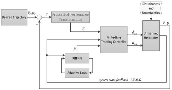
Figure 1. Overview of the control architecture.

3.1. Prescribed Performance Tracking Error Transformation

Define the original tracking errors as follows:

$$\left\{\begin{array}{c}{e}_P(t)=P(t)-P_d(t)\\ e_{\psi }(t)=\psi (t)-{\psi }_d(t)\end{array}\right.$$

(18)

Since Equation (9) is a typical inequality constraint, such form brings difficulties to the design of control schemes. To realize performance constraints as Equation (9), the above original errors will be transformed into new equivalent errors ${\overline{e}}_P(t)$ and ${\overline{e}}_{\psi }(t)$. In this paper, by designing a novel conversion function, Equation (9) can be transformed into an unconstrained form, which is beneficial to the controller design. The error transformation function can be defined as

$${\overline{e}}_{Pi}(t)=\kappa (e_{Pi}(t),{\rho }_i(t),{\sigma }_{Li}(t),{\sigma }_{Ui}(t))\hspace{1em}i=1,2,3$$

(19)

where ${\overline{e}}_{Pi}(t)$ is the new transformed tracking error of $e_{Pi}(t)$. By introducing a positive constant parameter ${\delta }_P$, ${\overline{e}}_{Pi}(t)$ can be concretely expressed as

$${\overline{e}}_{Pi}(t)={\displaystyle \frac{2e_{Pi}(t)-\left[P_{Ui}(t)+P_{Li}(t)\right]}{{\delta }_P^{-1}\left[P_{Ui}(t)-P_{Li}(t)\right]}}$$

(20)

Then, the Theorem 1 is given as follows.

Theorem 1.

If ${\overline{e}}_{Pi}(t)$ is bounded with $\left|{\overline{e}}_{Pi}(t)\right|<{\delta }_P$, the tracking error $e_{Pi}(t)$ will be confined within the preset prescribed bounds as Equation (9).

Proof. 

If the condition $\left|{\overline{e}}_{Pi}(t)\right|<{\delta }_P$ is maintained, combining Equation (16) yields

$$-{\delta }_P<{\displaystyle \frac{2e_{Pi}(t)-\left[P_{Ui}(t)+P_{Li}(t)\right]}{{\delta }_P^{-1}\left[P_{Ui}(t)-P_{Li}(t)\right]}}<{\delta }_P.$$

(21)

Since $P_{Ui}(t)>P_{Li}(t)$ and ${\delta }_P>0$, multiply both sides of Equation (21) by ${\delta }_P^{-1}\left[P_{Ui}(t)-P_{Li}(t)\right]$, one can easily obtain $P_{Li}(t)<e_{Pi}(t)<P_{Ui}(t)$.

This completes the proof of Theorem 1. □

Further, the differential of ${\overline{e}}_{Pi}(t)$ can be derived as

$${\dot{\overline{e}}}_{Pi}(t)={\displaystyle \frac{2{\dot{e}}_{Pi}(t)}{{\delta }_P^{-1}\left[P_{Ui}(t)-P_{Li}(t)\right]}}-2{\displaystyle \frac{e_{Pi}(t)\left[{\dot{P}}_{Ui}(t)-{\dot{P}}_{Li}(t)\right]+P_{Ui}(t){\dot{P}}_{Li}(t)-{\dot{P}}_{Ui}(t)P_{Li}(t)}{{\delta }_P^{-1}{\left[P_{Ui}(t)-P_{Li}(t)\right]}^2}}$$

(22)

where

$$\left\{\begin{array}{l}{\dot{P}}_{Li}(t)=-{\dot{\sigma }}_{Li}(t){\rho }_i(t)-{\sigma }_{Li}(t){\dot{\rho }}_i(t)\\ {\dot{P}}_{Ui}(t)={\dot{\sigma }}_{Ui}(t){\rho }_i(t)+{\sigma }_{Ui}(t){\dot{\rho }}_i(t)\\ {\dot{\rho }}_i(t)=-{\kappa }_i{\rho }_{i0}{\exp }^{-{\kappa }_{i}t}\end{array}\right.$$

(23)

Then, applying the above method to $e_{\psi }(t)$, the following results can be obtained

$$\left\{\begin{array}{l}{P}_{L\psi }(t)<e_{\psi }(t)<P_{L\psi }(t)\hfill \\ {\overline{e}}_{\psi }={\displaystyle \frac{2e_{\psi }(t)-\left[P_{U\psi }(t)+P_{L\psi }(t)\right]}{{\delta }_{\psi }^{-1}\left[P_{U\psi }(t)-P_{L\psi }(t)\right]}} \hfill \\ {\dot{\overline{e}}}_{\psi }={\displaystyle \frac{2{\dot{e}}_{\psi }(t)}{{\delta }_{\psi }^{-1}\left[P_{U\psi }(t)-P_{L\psi }(t)\right]}}-2{\displaystyle \frac{e_{\psi }(t)\left({\dot{P}}_{U\psi }-{\dot{P}}_{L\psi }\right)+P_{U\psi }(t){\dot{P}}_{L\psi }(t)-{\dot{P}}_{U\psi }(t)P_{L\psi }(t)}{{\delta }_{\psi }^{-1}{\left[P_{U\psi }(t)-P_{Li}(t)\right]}^2}}\hfill \end{array}\right.$$

(24)

where the relevant parameters are defined in a form similar to ${\overline{e}}_{Pi}(t)$.

To simplify the description, intermediate variables $M_{Pi}$, $N_{Pi}$, $m_{\psi }$ and $n_{\psi }$ are introduced as follows

$$\left\{\begin{array}{l}{M}_{Pi}(t)\triangleq {\displaystyle \frac{2{\delta }_P}{P_{Ui}(t)-P_{Li}(t)}}\\ N_{Pi}(t)\triangleq {\displaystyle \frac{-M_{Pi}}{P_{Ui}(t)-P_{Li}(t)}}\left[e_{Pi}(t)\left({\dot{P}}_{Ui}(t)-{\dot{P}}_{Li}(t)\right)+P_{Ui}(t){\dot{P}}_{Li}(t)-{\dot{P}}_{Ui}(t)P_{Li}(t)\right]\\ m_{\psi }(t)\triangleq {\displaystyle \frac{2{\delta }_{\psi }}{P_{U\psi }(t)-P_{L\psi }(t)}}\\ n_{\psi }(t)\triangleq {\displaystyle \frac{-m_{\psi }}{P_{U\psi }(t)-P_{L\psi }(t)}}\left[e_{\psi }(t)\left({\dot{P}}_{U\psi }(t)-{\dot{P}}_{L\psi }(t)\right)+P_{U\psi }(t){\dot{P}}_{L\psi }(t)-{\dot{P}}_{U\psi }(t)P_{L\psi }(t)\right]\end{array}\right.$$

(25)

Note that $\psi (t)=e_3^T\Theta (t)$, define ${\overline{e}}_{\Theta }=[e_{\varphi },e_{\theta },{\overline{e}}_{\psi }]$, $M_{\Theta }=diag\left(1,1,m_{\psi }\right)$ and $N_{\Theta }=n_{\psi }{e}_3$, then differentiating ${\overline{e}}_P$, ${\overline{e}}_{\Theta }$ and combining Equations (22), (24) and (25) can derive

$${\dot{\overline{e}}}_P(t)=M_{P}V+N_P-M_P{\dot{P}}_d$$

(26)

$${\dot{\overline{e}}}_{\Theta }(t)=M_{\Theta }\Pi (\Theta )\Omega +N_{\Theta }-M_{\Theta }{\dot{\Theta }}_d$$

(27)

where $M_P=diag(M_{Pi})$, $N_P={[N_{P1},N_{P2},N_{P3}]}^T$ and ${\Theta }_d$ is the ideal attitude control signal, which will be designed later.

Remark 3.

In particular, when the new transformed tracking error ${\overline{e}}_{Pi}(t)$ converges to zero, according to Equation (20), one can obtain

$$e_{Pi}(t)={\displaystyle \frac{1}{2}}\left[P_{Ui}(t)+P_{Li}(t)\right].$$

Obviously, $e_{Pi}(t)$ is still constrained within the boundaries $P_{Ui}(t)$ and $P_{Li}(t)$, and if $a=c$ and $b=d$ are selected, $P_{Ui}(t)$ and $P_{Li}(t)$ have already converged to the steady state boundaries ${\rho }_{\infty }b/a$ and $-{\rho }_{\infty }d/c$, respectively, then $e_{Pi}(t)$ will converge to zero.

3.2. Finite-Time Neural Network Disturbance Observer Design

To begin with, define the control errors as follows:

$$\left\{\begin{array}{c}{e}_V(t)=V(t)-V_d(t)\\ e_{\Omega }(t)=\Omega (t)-{\Omega }_d(t)\end{array}\right.$$

(28)

where $V_d(t)$ and ${\Omega }_d(t)$ are the virtual control to be designed below.

Simultaneous Equations (3) and (27), it follows

$$\left\{\begin{array}{l}{\dot{e}}_V(t)=g{e}_3-g{R}_3+A_{V}V+B_V{u}_{col}(t)+{\Lambda }_1{F}_1\\ {\dot{\overline{e}}}_{\Theta }(t)=M_{\Theta }\Pi (\Theta )\Omega +N_{\Theta }+{\Lambda }_2{F}_2\\ {\dot{e}}_{\Omega }(t)=-I_m^{-1}H\left(\Omega \right)I_m\Omega +A_{\Omega }\Omega +B_{\Omega }{u}_{res}+{\Lambda }_3{F}_3\end{array}\right.$$

(29)

where

$$\begin{array}{l}{\Lambda }_1={\Lambda }_3=I_3\\ {\Lambda }_2=diag\left(1,1,1-{\delta }_{\psi }^{-2}{e}_{\psi }^2\right)\\ F_1={\Lambda }_1^{-1}\left[d_1(t)-{\dot{V}}_d\right]\\ F_2=-{\Lambda }_2^{-1}{M}_{\Theta }{\dot{\Theta }}_d\\ F_3={\Lambda }_3^{-1}\left[d_2(t)-{\dot{\Omega }}_d\right]\end{array}.$$

In this study, the radial basis function RBFNN and adaptive laws are chosen to construct a finite-time NN observer for the estimation of lump disturbance $F$. The FTNNDO system is constructed as follows:

$$\left\{\begin{array}{l}{\dot{\widehat{e}}}_V(t)=g{e}_3-g{R}_3+A_{V}V+B_V{u}_{col}+{\Lambda }_1{\widehat{F}}_1(t)\\ {\dot{\widehat{e}}}_{\Theta }(t)=M_{\Theta }\Pi (\Theta )\Omega +{\Lambda }_2{\widehat{F}}_2(t)\\ {\dot{\widehat{e}}}_{\Omega }(t)=-I_m^{-1}H\left(\Omega \right)I_m\Omega +A_{\Omega }\Omega +B_{\Omega }{u}_{res}+{\Lambda }_3{\widehat{F}}_3(t)\\ {\widehat{F}}_i(t)={{\widehat{W}}_i}^T{h}_i({\chi }_i)+{\widehat{\epsilon }}_{iNN}\tanh (s_i/\varsigma )+{\iota }_{i1}{s}_i+{\iota }_{i2}{s_i}^r\end{array}\right.$$

(30)

where ${\widehat{e}}_V$, ${\widehat{e}}_{\Theta }$ and ${\widehat{e}}_{\Omega }$ are the estimates of $e_V$, ${\overline{e}}_{\Theta }$ and $e_{\Omega }$, respectively. $s_i,i=1,2,3$ are the observer errors, i.e., $s_1=e_V-{\widehat{e}}_V$, $s_2={\overline{e}}_{\Theta }-{\widehat{e}}_{\Theta }$, $s_3=e_{\Omega }-{\widehat{e}}_{\Omega }$. ${\widehat{\epsilon }}_{iNN}$ is the estimate of unknown NN error bound ${\epsilon }_{iNN}$. $\varsigma$, ${\iota }_{i1}$ and ${\iota }_{i2}$ are the designed positive constants, and $r$ is defined as $0<r=p_r/q_r$ with $p_r$ and $q_r$ being positive odd integers and satisfying $p_r<q_r$.

The structure of the FTNNDO is shown in Figure 2. There are three layers in the RBFNN: an input layer, a hidden layer with the nonlinear NN activation function $h_i({\chi }_i)$ and a linear output layer.

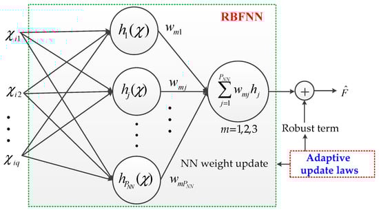
Figure 2. Structure of the FTNNDO.

The input layer $\chi$ contains the command control signals and system states related to the unknown function $F$. Severally, ${\chi }_1$ is composed of ($P$, $V$, $V_d$, $u_{col}$), ${\chi }_2$ is composed of ($\Theta$, $\Omega$, ${\Theta }_d$), and ${\chi }_3$ is composed of ($\Theta$, $\Omega$, ${\Omega }_d$, $u_{res}$). The hidden layer consists of multiple radial basis functions, which are Gaussian basis functions designed as Equation (5). By combining the robust term ${\iota }_{1}s+{\iota }_2{s}^r+{\widehat{\epsilon }}_{NN}\tanh (s/\varsigma )$ and updating the weight matrix $\widehat{W}$ between the hidden layer and the output layer, the FTNNDO can finally generate the approximation of $F$ with a very small approximate error.

The adaptive law for updating NN is designed as

$${\dot{\widehat{W}}}_i={\Gamma }_i\left[h_i({\chi }_i){s_i}^T{\Lambda }_i-{\sigma }_{iNN}{{\Gamma }_i}^{-1}{\widehat{W}}_i\right]$$

(31)

where ${\Gamma }_i$ is the NN learning gain matrix to be designed, and ${\sigma }_{iNN}>0.$

The adaptive law for updating ${\widehat{\epsilon }}_{iNN}$ is designed as

$${\dot{\widehat{\epsilon }}}_{iNN}=-{\beta }_i{\widehat{\epsilon }}_{iNN}+{s_i}^T{\Lambda }_i\tanh (s_i/\varsigma )$$

(32)

where ${\beta }_i>0.$

Combining Equations (29) and (30), the derivative of $s_i$ can be described as follows:

$$\left\{\begin{array}{c}{\dot{s}}_1={\dot{e}}_V-{\dot{\widehat{e}}}_V={\Lambda }_1{\tilde{F}}_1\\ {\dot{s}}_2={\dot{\overline{e}}}_{\Theta }-{\dot{\widehat{e}}}_{\Theta }={\Lambda }_2{\tilde{F}}_2\\ {\dot{s}}_3={\dot{e}}_{\Omega }-{\dot{\widehat{e}}}_{\Omega }={\Lambda }_3{\tilde{F}}_3\end{array}\right.$$

(33)

Obviously, ${\dot{s}}_i$ contains the information of ${\tilde{F}}_i$, which can be used to indicate the convergence of the estimation error of the lump disturbance. Defining the weight vector error as ${\tilde{W}}_i=W_i^{*}-{\widehat{W}}_i$, ${\tilde{F}}_i$ can be calculated as

$$\begin{array}{ll}{\tilde{F}}_i& =F_i-{\widehat{F}}_i\\ & ={{\tilde{W}}_i}^T{h}_i({\chi }_i)+{\epsilon }_i-{\widehat{\epsilon }}_{iNN}\tanh (s_i/\varsigma )-{\iota }_{i1}{s}_i-{\iota }_{i2}{s_i}^r\end{array}$$

(34)

Theorem 2.

Consider system Equation (29), if the FTNNDO is designed as Equation (30) and the adaptive laws are set to be Equations (31) and (32), then, all closed-loop system signals are bounded in finite time, as well as the observation errors $s_i$, ${\tilde{W}}_i$, ${\tilde{\epsilon }}_{iNN}$ and ${\tilde{F}}_i$ will converge into the disc regions with a sufficiently small radius in finite time.

Proof. 

The FTNNDO is composed of three subsystems with the same structure. Consider a Lyapunov function candidate as

$${\dot{L}}_O={\displaystyle \sum _{i=1}^n{\dot{L}}_{Oi}}\hspace{1em}n=3$$

(35)

Suppose the NN estimation error ${\epsilon }_i$ is bound, there exists a positive unknown bound ${\epsilon }_{iNN}$ such that $\left|{\epsilon }_i\right|\le {\epsilon }_{iNN}$. Define ${\tilde{\epsilon }}_{iNN}={\epsilon }_{iNN}-{\widehat{\epsilon }}_{iNN}$. For the observer subsystem, $L_{Oi}$ is described as

$$L_{Oi}={\displaystyle \frac{1}{2}}{s_i}^T{s}_i+{\displaystyle \frac{1}{2}}{\tilde{\epsilon }}_{iNN}^T{\tilde{\epsilon }}_{iNN}+{\displaystyle \frac{1}{2}}tr({{\tilde{W}}_i}^T{{\Gamma }_i}^{-1}{\tilde{W}}_i)$$

(36)

where $tr(•)$ denotes the matrix trace.

Substituting Equations (31)–(33) into Equation (36) yields

$$\begin{array}{ll}{\dot{L}}_{O_i}& ={s_i}^T{\dot{s}}_i+{\tilde{\epsilon }}_{iNN}^T{\dot{\tilde{\epsilon }}}_{iNN}+tr({{\tilde{W}}_i}^T{{\Gamma }_i}^{-1}{\dot{\tilde{W}}}_i)\\ & ={s_i}^T{\Lambda }_i\left[{{\tilde{W}}_i}^T{h}_i({\chi }_i)+{\epsilon }_i-{\epsilon }_{iNN}\tanh (s_i/\varsigma )+{\tilde{\epsilon }}_{iNN}\tanh (s_i/\varsigma )-{\iota }_{i1}{s}_i-{\iota }_{i2}{s_i}^r\right]\\ & +{\tilde{\epsilon }}_{iNN}^T\left[{\beta }_i{\widehat{\epsilon }}_{iNN}+{s_i}^T{\Lambda }_i\tanh (s_i/\varsigma )\right]-tr({{\tilde{W}}_i}^T{h}_i({\chi }_i){s_i}^T{\Lambda }_i-{\sigma }_{iNN}{{\tilde{W}}_i}^T{{\Gamma }_i}^{-1}{\widehat{W}}_i)\\ & ={s_i}^T{\Lambda }_i{{\tilde{W}}_i}^T{h}_i({\chi }_i)+{s_i}^T{\Lambda }_i\left[{\epsilon }_i-{\epsilon }_{iNN}\tanh (s_i/\varsigma )\right]-{\iota }_{i1}{s_i}^T{s}_i-{\iota }_{i2}{s_i}^T{s_i}^r\\ & +{\beta }_i{\tilde{\epsilon }}_{iNN}^T{\widehat{\epsilon }}_{iNN}-tr({\Lambda }_i{{\tilde{W}}_i}^T{h}_i({\chi }_i){s_i}^T)+tr({\sigma }_{iNN}{{\tilde{W}}_i}^T{{\Gamma }_i}^{-1}{\widehat{W}}_i)\end{array}.$$

(37)

According to ${s_i}^T{\Lambda }_i{{\tilde{W}}_i}^T{h}_i(\chi )=tr({{\tilde{W}}_i}^T{h}_i(\chi ){s_i}^T{\Lambda }_i)$, one can obtain

$$\begin{array}{ll}{\dot{L}}_{O_i}& ={s_i}^T{\Lambda }_i\left[{\epsilon }_i-{\epsilon }_{iNN}\tanh (s_i/\varsigma )\right]-{\iota }_{i1}{s_i}^T{\Lambda }_i{s}_i-{\iota }_{i2}{s_i}^T{\Lambda }_i{s_i}^r\\ & +{\beta }_i{\tilde{\epsilon }}_{iNN}^T{\widehat{\epsilon }}_{iNN}+{\sigma }_{iNN}tr({{\tilde{W}}_i}^T{{\Gamma }_i}^{-1}{\widehat{W}}_i)\\ & \le {\displaystyle \sum _{j=1}^n\left[{\Lambda }_{ij}\left|s_{ij}\right|\left|{\epsilon }_i\right|-{\Lambda }_{ij}{s}_{ij}{\epsilon }_{iNN}\tanh (s_{ij}/\varsigma )\right]}{s_i}^T\tanh (s_i/\varsigma )-{\iota }_{i1}{s_i}^T{\Lambda }_i{s}_i-{\iota }_{i2}{s_i}^T{\Lambda }_i{s_i}^r\\ & +{\beta }_i{\tilde{\epsilon }}_{iNN}^T{\widehat{\epsilon }}_{iNN}+{\sigma }_{iNN}tr({{\tilde{W}}_i}^T{{\Gamma }_i}^{-1}{\widehat{W}}_i)\\ & \le {\epsilon }_{iNN}{\displaystyle \sum _{j=1}^n{\Lambda }_{ij}\left[\left|s_{ij}\right|-s_{ij}\tanh (s_{ij}/\varsigma )\right]}-{\iota }_{i1}{s_i}^T{\Lambda }_i{s}_i-{\iota }_{i2}{s_i}^T{\Lambda }_i{s_i}^r\\ & +{\beta }_i{\tilde{\epsilon }}_{iNN}^T{\widehat{\epsilon }}_{iNN}+{\sigma }_{iNN}tr({{\tilde{W}}_i}^T{{\Gamma }_i}^{-1}{\widehat{W}}_i)\end{array}.$$

(38)

Using Lemma 3 and the inequalities as follows

$$\left\{\begin{array}{l}{\tilde{\epsilon }}_{iNN}^T{\widehat{\epsilon }}_{iNN}\le -{\displaystyle \frac{1}{2}}{\tilde{\epsilon }}_{iNN}^T{\tilde{\epsilon }}_{iNN}+{\displaystyle \frac{1}{2}}{\epsilon }_{iNN}^T{\epsilon }_{iNN}\hfill \\ tr({{\tilde{W}}_i}^T{{\Gamma }_i}^{-1}{\widehat{W}}_i)\le -{\displaystyle \frac{1}{2}}tr({{\tilde{W}}_i}^T{{\Gamma }_i}^{-1}{\tilde{W}}_i)+{\displaystyle \frac{1}{2}}tr({W_i}^{*T}{{\Gamma }_i}^{-1}{W_i}^{*})\hfill \\ 0<{\Lambda }_{ij}\le 1\hfill \end{array}\right.$$

(39)

can derive

$$\begin{array}{ll}{\dot{L}}_{Oi}& \le 0.2785n\varsigma {\epsilon }_{iNN}-{\iota }_{i1}{s_i}^T{\Lambda }_i{s}_i-{\iota }_{i2}{s_i}^T{\Lambda }_i{s_i}^r-{\displaystyle \frac{{\beta }_i}{2}}{\tilde{\epsilon }}_{iNN}^T{\tilde{\epsilon }}_{iNN}+{\displaystyle \frac{{\beta }_i}{2}}{\epsilon }_{iNN}^T{\epsilon }_{iNN}\\ & -{\displaystyle \frac{{\sigma }_{iNN}}{2}}tr({{\tilde{W}}_i}^T{{\Gamma }_i}^{-1}{\tilde{W}}_i)+{\displaystyle \frac{{\sigma }_{iNN}}{2}}tr({W_i}^{*T}{{\Gamma }_i}^{-1}{W_i}^{*})\\ & \le {\iota }_{i1}{s_i}^T{\Lambda }_i{s}_i-{\iota }_{i2}{s_i}^T{\Lambda }_i{s_i}^r-{\displaystyle \frac{{\beta }_i}{2}}{\tilde{\epsilon }}_{iNN}^T{\tilde{\epsilon }}_{iNN}-{\displaystyle \frac{{\sigma }_{i1}}{2}}{\left({\tilde{\epsilon }}_{iNN}^T{\tilde{\epsilon }}_{iNN}\right)}^{{\displaystyle \frac{r+1}{2}}}\\ & -{\displaystyle \frac{{\sigma }_{iNN}}{2}}tr({{\tilde{W}}_i}^T{{\Gamma }_i}^{-1}{\tilde{W}}_i)-{\displaystyle \frac{{\sigma }_{i2}}{2}}tr{({{\tilde{W}}_i}^T{{\Gamma }_i}^{-1}{\tilde{W}}_i)}^{{\displaystyle \frac{r+1}{2}}}\\ & +{\displaystyle \frac{{\sigma }_{i1}}{2}}{\left({\tilde{\epsilon }}_{iNN}^T{\tilde{\epsilon }}_{iNN}\right)}^{{\displaystyle \frac{r+1}{2}}}+{\displaystyle \frac{{\sigma }_{i2}}{2}}tr{({{\tilde{W}}_i}^T{{\Gamma }_i}^{-1}{\tilde{W}}_i)}^{{\displaystyle \frac{r+1}{2}}}\\ & +{\displaystyle \frac{{\beta }_i}{2}}{\epsilon }_{iNN}^T{\epsilon }_{iNN}+{\displaystyle \frac{{\sigma }_{iNN}}{2}}tr({W_i}^{*T}{{\Gamma }_i}^{-1}{W_i}^{*})+0.2785n\varsigma {\epsilon }_{iNN}\\ & \le -{\iota }_{i1}{\lambda }_{\min }\left({\Lambda }_i\right){\left|s_i\right|}^2-{\iota }_{i2}{\lambda }_{\min }\left({\Lambda }_i\right){\left|s_i\right|}^{r+1}-{\displaystyle \frac{{\beta }_i}{2}}{\left|{\tilde{\epsilon }}_{iNN}\right|}^2-{\displaystyle \frac{{\sigma }_{i1}}{2}}{\left|{\tilde{\epsilon }}_{iNN}\right|}^{r+1}\\ & -{\displaystyle \frac{{\sigma }_{iNN}}{2}}tr({{\tilde{W}}_i}^T{{\Gamma }_i}^{-1}{\tilde{W}}_i)-{\displaystyle \frac{{\sigma }_{i2}}{2}}tr{({{\tilde{W}}_i}^T{{\Gamma }_i}^{-1}{\tilde{W}}_i)}^{{\displaystyle \frac{r+1}{2}}}\\ & +{\displaystyle \frac{{\sigma }_{i1}}{2}}{\left|{\tilde{\epsilon }}_{NN}\right|}^{r+1}+{\displaystyle \frac{{\sigma }_{i2}}{2}}{\lambda }_{\max }{({{\Gamma }_i}^{-1})}^{{\displaystyle \frac{r+1}{2}}}{\left|{\tilde{W}}_i\right|}^{r+1}\\ & +{\displaystyle \frac{{\beta }_i}{2}}{\left|{\epsilon }_{iNN}\right|}^2+{\displaystyle \frac{{\sigma }_{iNN}}{2}}tr({W_i}^{*T}{{\Gamma }_i}^{-1}{W_i}^{*})+0.2785n\varsigma {\epsilon }_{iNN}\end{array}$$

(40)

Using Lemma 4 and choosing ${\gamma }_1$ and ${\gamma }_2$ as

$$\left\{\begin{array}{l}{\gamma }_1={\left({\displaystyle \frac{r+1}{2}}\right)}^{{\displaystyle \frac{r+1}{1-r}}}\\ {\gamma }_2={\left({\displaystyle \frac{r+1}{2}}\right)}^{{\displaystyle \frac{r+1}{1-r}}}{\lambda }_{\max }^{-{\displaystyle \frac{r+1}{1-r}}}({{\Gamma }_i}^{-1})\end{array}\right.$$

(41)

can obtain

$$\begin{array}{ll}{\left|{\tilde{\epsilon }}_{iNN}\right|}^{r+1}& =1^{1-r}{\left|{\tilde{\epsilon }}_{iNN}\right|}^{r+1}\\ & \le {\displaystyle \frac{1-r}{2}}{\gamma }_1+{\displaystyle \frac{r+1}{2}}{\gamma }_1^{-{\displaystyle \frac{1-r}{r+1}}}{\left|{\tilde{\epsilon }}_{iNN}\right|}^2\\ & <{\left|{\tilde{\epsilon }}_{iNN}\right|}^2+{\displaystyle \frac{1}{4}}\end{array}$$

(42)

$$\begin{array}{ll}{\lambda }_{\max }{({{\Gamma }_i}^{-1})}^{{\displaystyle \frac{r+1}{2}}}{\left|{\tilde{W}}_i\right|}^{r+1}& ={\left[{\lambda }_{\max }^{{\displaystyle \frac{r+1}{2(1-r)}}}({{\Gamma }_i}^{-1})\right]}^{1-r}{‖{\tilde{W}}_i‖}^{r+1}\\ & \le {\displaystyle \frac{1-r}{2}}{\gamma }_2{\lambda }_{\max }^{{\displaystyle \frac{r+1}{1-r}}}({{\Gamma }_i}^{-1})+{\displaystyle \frac{r+1}{2}}{\gamma }_2^{-{\displaystyle \frac{1-r}{r+1}}}{‖{\tilde{W}}_i‖}^2\\ & \le {\displaystyle \frac{1-r}{2}}{\left({\displaystyle \frac{r+1}{2}}\right)}^{{\displaystyle \frac{r+1}{1-r}}}+{\lambda }_{\max }({{\Gamma }_i}^{-1}){‖{\tilde{W}}_i‖}^2\\ & <{\displaystyle \frac{1}{4}}+{\displaystyle \frac{{\lambda }_{\max }({{\Gamma }_i}^{-1})}{{\lambda }_{\min }({{\Gamma }_i}^{-1})}}tr({{\tilde{W}}_i}^T{{\Gamma }_i}^{-1}{\tilde{W}}_i)\end{array}$$

(43)

Substituting Equations (42) and (43) into Equation (40) can obtain

$$\begin{array}{ll}{\dot{L}}_{Oi}& <-{\iota }_{i1}{\lambda }_{\min }\left({\Lambda }_i\right){\left|s_i\right|}^2-{\iota }_{i2}{\lambda }_{\min }\left({\Lambda }_i\right){\left|s_i\right|}^{r+1}-{\displaystyle \frac{{\beta }_i-{\sigma }_{i1}}{2}}{\left|{\tilde{\epsilon }}_{iNN}\right|}^2-{\displaystyle \frac{{\sigma }_{i1}}{2}}{\left|{\tilde{\epsilon }}_{iNN}\right|}^{r+1}\\ & -\left[{\displaystyle \frac{{\sigma }_{iNN}}{2}}-{\displaystyle \frac{{\sigma }_{i2}}{2}}{\displaystyle \frac{{\lambda }_{\max }({{\Gamma }_i}^{-1})}{{\lambda }_{\min }({{\Gamma }_i}^{-1})}}\right]tr({{\tilde{W}}_i}^T{{\Gamma }_i}^{-1}{\tilde{W}}_i)-{\displaystyle \frac{{\sigma }_{i2}}{2}}tr{({{\tilde{W}}_i}^T{{\Gamma }_i}^{-1}{\tilde{W}}_i)}^{{\displaystyle \frac{r+1}{2}}}\\ & +{\displaystyle \frac{{\beta }_i}{2}}{\left|{\epsilon }_{iNN}\right|}^2+{\displaystyle \frac{{\sigma }_{iNN}}{2}}tr({W_i}^{*T}{{\Gamma }_i}^{-1}{W_i}^{*})+0.2785n\varsigma {\epsilon }_{NN}+{\displaystyle \frac{{\sigma }_{i1}+{\sigma }_{i2}}{8}}\\ & <-2\min \left\{{\iota }_{i1}{\lambda }_{\min }\left({\Lambda }_i\right),{\displaystyle \frac{{\beta }_i-{\sigma }_{i1}}{2}},{\displaystyle \frac{{\sigma }_{iNN}}{2}}-{\displaystyle \frac{{\sigma }_{i2}}{2}}{\displaystyle \frac{{\lambda }_{\max }({{\Gamma }_i}^{-1})}{{\lambda }_{\min }({{\Gamma }_i}^{-1})}}\right\}\left[{\displaystyle \frac{1}{2}}{\left|s_i\right|}^2+{\displaystyle \frac{1}{2}}{\left|{\tilde{\epsilon }}_{iNN}\right|}^2+{\displaystyle \frac{1}{2}}tr({{\tilde{W}}_i}^T{{\Gamma }_i}^{-1}{\tilde{W}}_i)\right]\\ & -\min \left\{{\iota }_{i2}{\lambda }_{\min }\left({\Lambda }_i\right),{\displaystyle \frac{{\sigma }_{i1}}{2}},{\displaystyle \frac{{\sigma }_{i2}}{2}}\right\}\left[{\left|s_i\right|}^{r+1}+{\left|{\tilde{\epsilon }}_{iNN}\right|}^{r+1}+tr{({{\tilde{W}}_i}^T{{\Gamma }_i}^{-1}{\tilde{W}}_i)}^{{\displaystyle \frac{r+1}{2}}}\right]\\ & +{\displaystyle \frac{{\beta }_i}{2}}{\left|{\epsilon }_{iNN}\right|}^2+{\displaystyle \frac{{\sigma }_{iNN}}{2}}tr({W_i}^{*T}{{\Gamma }_i}^{-1}{W_i}^{*})+0.2785n\varsigma {\epsilon }_{iNN}+{\displaystyle \frac{{\sigma }_{i1}+{\sigma }_{i2}}{8}}\end{array}$$

(44)

Further, using Lemma 2 yields

$$\begin{array}{l}{\left|s_i\right|}^{r+1}+{\left|{\tilde{\epsilon }}_{iNN}\right|}^{r+1}+tr{({{\tilde{W}}_i}^T{{\Gamma }_i}^{-1}{\tilde{W}}_i)}^{{\displaystyle \frac{r+1}{2}}}\\ ={\left({\left|s_i\right|}^2\right)}^{{\displaystyle \frac{r+1}{2}}}+{\left({\left|{\tilde{\epsilon }}_{iNN}\right|}^2\right)}^{{\displaystyle \frac{r+1}{2}}}+tr{({{\tilde{W}}_i}^T{{\Gamma }_i}^{-1}{\tilde{W}}_i)}^{{\displaystyle \frac{r+1}{2}}}\\ \ge {\left({\left|s_i\right|}^2+{\left|{\tilde{\epsilon }}_{iNN}\right|}^2+tr({{\tilde{W}}_i}^T{{\Gamma }_i}^{-1}{\tilde{W}}_i)\right)}^{{\displaystyle \frac{r+1}{2}}}\end{array}$$

(45)

Then, one can obtain

$$\begin{array}{ll}{\dot{L}}_{Oi}& <-2\min \left\{{\iota }_{i1}{\lambda }_{\min }\left({\Lambda }_i\right),{\displaystyle \frac{{\beta }_i-{\sigma }_{i1}}{2}},{\displaystyle \frac{{\sigma }_{iNN}}{2}}-{\displaystyle \frac{{\sigma }_{i2}}{2}}{\displaystyle \frac{{\lambda }_{\max }({{\Gamma }_i}^{-1})}{{\lambda }_{\min }({{\Gamma }_i}^{-1})}}\right\}\left[{\displaystyle \frac{1}{2}}{\left|s_i\right|}^2+{\displaystyle \frac{1}{2}}{\left|{\tilde{\epsilon }}_{iNN}\right|}^2+{\displaystyle \frac{1}{2}}tr({{\tilde{W}}_i}^T{{\Gamma }_i}^{-1}{\tilde{W}}_i)\right]\\ & -\min \left\{{\iota }_{i2}{\lambda }_{\min }\left({\Lambda }_i\right),{\displaystyle \frac{{\sigma }_{i1}}{2}},{\displaystyle \frac{{\sigma }_{i2}}{2}}\right\}{\left({\left|s_i\right|}^2+{\left|{\tilde{\epsilon }}_{iNN}\right|}^2+tr({{\tilde{W}}_i}^T{{\Gamma }_i}^{-1}{\tilde{W}}_i)\right)}^{{\displaystyle \frac{r+1}{2}}}\\ & +{\displaystyle \frac{{\beta }_i}{2}}{‖{\epsilon }_{NN}‖}^2+{\displaystyle \frac{{\sigma }_{iNN}}{2}}tr({W_i}^{*T}{{\Gamma }_i}^{-1}{W_i}^{*})+0.2785n\varsigma {\epsilon }_{iNN}+{\displaystyle \frac{{\sigma }_{i1}+{\sigma }_{i2}}{8}}\\ & <-2\min \left\{{\iota }_{i1}{\lambda }_{\min }\left({\Lambda }_i\right),{\displaystyle \frac{{\beta }_i-{\sigma }_{i1}}{2}},{\displaystyle \frac{{\sigma }_{iNN}}{2}}-{\displaystyle \frac{{\sigma }_{i2}}{2}}{\displaystyle \frac{{\lambda }_{\max }({{\Gamma }_i}^{-1})}{{\lambda }_{\min }({{\Gamma }_i}^{-1})}}\right\}{L}_{oi}\\ & -2^{{\displaystyle \frac{r+1}{2}}}\min \left\{{\iota }_{i2}{\lambda }_{\min }\left({\Lambda }_i\right),{\displaystyle \frac{{\sigma }_{i1}}{2}},{\displaystyle \frac{{\sigma }_{i2}}{2}}\right\}{L}_{oi}^{{\displaystyle \frac{r+1}{2}}}\\ & +{\displaystyle \frac{{\beta }_i}{2}}{‖{\epsilon }_{NN}‖}^2+{\displaystyle \frac{{\sigma }_{iNN}}{2}}tr({W_i}^{*T}{{\Gamma }_i}^{-1}{W_i}^{*})+0.2785n\varsigma {\epsilon }_{iNN}+{\displaystyle \frac{{\sigma }_{i1}+{\sigma }_{i2}}{8}}\\ & <-c_{i1}{L}_{oi}-c_{i2}{L}_{oi}^{{\displaystyle \frac{r+1}{2}}}+C_i\end{array}$$

(46)

where

$$\begin{array}{l}{c}_{i1}=\min \left\{2{\iota }_{i1}{\lambda }_{\min }\left({\Lambda }_i\right),{\beta }_i-{\sigma }_{i1},{\sigma }_{iNN}-{\displaystyle \frac{{\sigma }_{i2}{\lambda }_{\max }({{\Gamma }_i}^{-1})}{{\lambda }_{\min }({{\Gamma }_i}^{-1})}}\right\}\\ c_{i2}=2^{{\displaystyle \frac{r+1}{2}}}\min \left\{{\iota }_{i2}{\lambda }_{\min }\left({\Lambda }_i\right),{\displaystyle \frac{{\sigma }_{i1}}{2}},{\displaystyle \frac{{\sigma }_{i2}}{2}}\right\}\\ C_i={\displaystyle \frac{{\beta }_i}{2}}{‖{\epsilon }_{NN}‖}^2+{\displaystyle \frac{{\sigma }_{iNN}}{2}}tr({W_i}^{*T}{{\Gamma }_i}^{-1}{W_i}^{*})+0.2785n\varsigma {\epsilon }_{iNN}+{\displaystyle \frac{{\sigma }_{i1}+{\sigma }_{i2}}{8}}\end{array}$$

Finally,

$$\begin{array}{ll}{\dot{L}}_O& ={\displaystyle \sum _{i=1}^n{\dot{L}}_{Oi}}\\ & \le -c_1{\displaystyle \sum _{i=1}^n{L}_{oi}}-c_2{\displaystyle \sum _{i=1}^n{L}_{oi}^{\frac{r+1}{2}}}+{\displaystyle \sum _{i=1}^n{C}_i}\\ & \le -c_1{L}_o-c_2{L}_o^{{\displaystyle \frac{r+1}{2}}}+C_o\end{array}$$

(47)

where

$$\begin{array}{l}{c}_1=n\min \left\{c_{i1}\right\}\\ c_2=n\min \left\{c_{i2}\right\}\\ C_o={\displaystyle \sum _{i=1}^n{C}_i}\end{array}$$

Choose

$${\iota }_{i1}>0,{\iota }_{i2}>0,{\beta }_i>{\sigma }_{i1}>0,{\sigma }_{iNN}>{\displaystyle \frac{{\lambda }_{\max }({{\mathrm{\Gamma }}_i}^{-1})}{{\lambda }_{\min }({\mathrm{\Gamma }}_i{-1}^{-1})}}{\sigma }_{i2}>0$$

According to Lemma 1, in finite time $T_r$, the bound of the FMNNDO estimation error will be very small.

$$T_r\le \max \left\{\begin{array}{l}{\displaystyle \frac{1}{{\theta }_0{c}_1(1-\frac{r+1}{2})}}\ln {\displaystyle \frac{{\theta }_0{c}_1{L_o}^{1-\frac{r+1}{2}}(0)+c_2}{c_2}},\\ {\displaystyle \frac{1}{c_1(1-\frac{r+1}{2})}}\ln {\displaystyle \frac{c_1{L_o}^{1-\frac{r+1}{2}}(0)+{\theta }_0{c}_2}{{\theta }_0{c}_2}}\end{array}\right\}$$

Moreover, the convergence regions of estimation errors are given as follows:

$$\begin{array}{l}\left|s_i\right|\le \min \left\{\sqrt{{\displaystyle \frac{2C_o}{\left(1-{\theta }_0\right)c_1}}},\sqrt{2{\left[{\displaystyle \frac{C_o}{\left(1-{\theta }_0\right)c_2}}\right]}^{{\displaystyle \frac{2}{r+1}}}}\right\}\\ \left|{\tilde{\epsilon }}_{iNN}\right|\le \min \left\{\sqrt{{\displaystyle \frac{2C_o}{\left(1-{\theta }_0\right)c_1}}},\sqrt{2{\left[{\displaystyle \frac{C_o}{\left(1-{\theta }_0\right)c_2}}\right]}^{{\displaystyle \frac{2}{r+1}}}}\right\}\\ ‖{\tilde{W}}_i‖\le \min \left\{\sqrt{{\displaystyle \frac{2C_o}{{\lambda }_{\min }({\Gamma }^{-1})\left(1-{\theta }_0\right)c_1}}},\sqrt{{\displaystyle \frac{2}{{\lambda }_{\min }({\Gamma }^{-1})}}{\left[{\displaystyle \frac{C_o}{\left(1-{\theta }_0\right)c_2}}\right]}^{{\displaystyle \frac{2}{r+1}}}}\right\}\end{array}$$

Distinctly, by choosing appropriate values of ${\iota }_{i1}$, ${\iota }_{i2}$, ${\sigma }_{i1}$, ${\sigma }_{i2}$, ${\beta }_i$, ${\sigma }_{iNN}$ and $\varsigma$, the regions can be sufficiently small. Noting that $h_i({\chi }_i)$ and $\tanh (s_i/\varsigma )$ are both bounded functions in Equation (39), hence ${\tilde{F}}_i(t)$ is also bounded with ${\varpi }_{Fi}$ and will converge to a small neighborhood ${\varpi }_i$ in finite time as

$$‖{\tilde{F}}_i(t)‖\le {\varpi }_i$$

(48)

This concludes the proof of Theorem 2. □

Remark 4.

The overall performance of the control system is closely related to the convergence rate of the observer, and a natural idea is that reducing the convergence time of observer estimation can improve the control performance and suppress the influence of external interference more quickly. Compared with previous results in [27,29,31], the proposed observer in this paper can converge faster in finite time. The hyperbolic tangent function is chosen to construct a continuous adaptive law such that the chattering phenomenon caused by the sign function in [33] can be eliminated. Different from the method in [34], which estimates the gain of the robust term for the NN approximation error as a large constant, the adaptive law designed in this paper can effectively estimate the upper bound of the NN error and compensate for the disturbance observer, thus avoiding the oscillation caused by the overestimation of the gain and improving the robustness. Moreover, the FTNNDO design and controller design can be carried out separately, so the FTNNDO in this paper can be easily integrated with other type control laws, which is very flexible.

Remark 5.

The parameters of FTNNDO mainly include NN structure parameters ( $b_{NN}$, $c_{NN}$, $P_{NN}$), adaptive law parameters (${\Gamma }_i$, ${\sigma }_{iNN}$, ${\beta }_i$, $\varsigma$) and other design parameters (${\iota }_{i1}$, ${\iota }_{i2}$, $r$). $b_{NN}$ and $c_{NN}$ can affect the performance of the Gaussian basis function $h(\chi )$. If the selected parameters are too large, $h(\chi )$ will be too sensitive to $\chi$; otherwise, the mapping ability of $h(\chi )$ will be poor. Empirically, $b_{NN}$ can be set to the maximum value of $\chi$, and $c_{NN}$ can be selected as $-b_{NN}+2b_{NN}i/(p_{NN}-1),i=0,1,\dots p_{NN}-1$. Increasing $P_{NN}$ can enhance the approximation accuracy, while reducing $P_{NN}$ can greatly reduce the NN calculation burden. Therefore, a good balance should be made through simulation training or a trial-and-error procedure. The update law parameters ${\Gamma }_i$, ${\sigma }_{iNN}$, ${\beta }_i$ and $\varsigma$ will affect the update speed of${\widehat{\epsilon }}_{iNN}$ and the NN weight matrix $\widehat{W}$. In general, the initial values of $\widehat{W}$ and ${\widehat{\epsilon }}_{iNN}$ are set to zero, while the NN learning rate ${\sigma }_{NN}$ is chosen from set $(0,1)$. The other parameters ${\iota }_{i1}$, ${\iota }_{i2}$ and $r$ affect the convergence rate of the FTNNDO, which also needs to be tuned appropriately via several simulations.

3.3. Finite-Time Tracking Controller Design and Stability Analysis

In the above sections, the prescribed performance function and FTNNDO have been developed to deal with the constrained tracking errors and the lumped disturbance of the system. Based on the above design and using the BLF, a composite finite-time tracking controller is designed to achieve the two control objectives proposed in this paper. The desired tracking controller can be obtained through the following design steps:

• Step 1: For the position tracking error dynamic in Equation (26), choose the virtual control signal $V_d$ as follows:

$$V_d=M_P^{-1}\left(-k_{P1}{\overline{e}}_P-k_{P2}{\left({\displaystyle \frac{1}{{\delta }_P^2-{\overline{e}}_{Pi}^2}}\right)}^{{\displaystyle \frac{r-1}{2}}}{\overline{e}}_P^r-N_P+M_P{\dot{P}}_d\right)$$

(49)

where $k_{P1}$ and $k_{P2}$ are positive constants to be designed.

To handle the prescribed performance, a barrier Lyapunov function $L_P$ is designed as

$$L_P={\displaystyle \frac{1}{2}}\log \left({\displaystyle \prod _{i=1}^3\frac{{\delta }_P^2}{{\delta }_P^2-{\overline{e}}_{Pi}^2}}\right)$$

(50)

where the value of ${\delta }_P$ is the same as that in the error conversion function, Equation (20).

Invoking Equations (26) and (49) and taking the derivative of $L_P$ can yield

$$\begin{array}{ll}{\dot{L}}_P& ={\displaystyle \sum _{i=1}^3\frac{{\overline{e}}_{Pi}{\dot{\overline{e}}}_{Pi}}{{\delta }_P^2-{\overline{e}}_{Pi}^2}}\\ & ={\overline{e}}_P^{T}diag\left({\displaystyle \frac{1}{{\delta }_P^2-{\overline{e}}_{Pi}^2}}\right)\left[M_P\left(V_d+e_V\right)-M_P{\dot{P}}_d+N_P\right]\\ & =-k_{P1}{\overline{e}}_P^{T}diag\left({\displaystyle \frac{1}{{\delta }_P^2-{\overline{e}}_{Pi}^2}}\right){\overline{e}}_P-k_{P2}{\overline{e}}_P^{T}diag{\left({\displaystyle \frac{1}{{\delta }_P^2-{\overline{e}}_{Pi}^2}}\right)}^{{\displaystyle \frac{r+1}{2}}}{{\overline{e}}_P}^r+{\overline{e}}_P^{T}diag\left({\displaystyle \frac{1}{{\delta }_P^2-{\overline{e}}_{Pi}^2}}\right)M_P{e}_V\\ & =-k_{P1}{\displaystyle \sum _{i=1}^3\frac{{\overline{e}}_{Pi}^2}{{\delta }_P^2-{\overline{e}}_{Pi}^2}}-k_{P2}{{\displaystyle \sum _{i=1}^3\left(\frac{{\overline{e}}_{Pi}^2}{{\delta }_P^2-{\overline{e}}_{Pi}^2}\right)}}^{{\displaystyle \frac{r+1}{2}}}+{\overline{e}}_P^{T}diag\left({\displaystyle \frac{1}{{\delta }_P^2-{\overline{e}}_{Pi}^2}}\right)M_P{e}_V\end{array}$$

(51)

• Step 2: For the velocity tracking error dynamic in Equation (28), choose the virtual control signal $u_{col}$ as follows:

$$u_{col}={B_V}^{-1}\left[-k_{V1}{e}_V-k_{V2}{e}_V^r+g{R}_3-g{e}_3-A_{V}V-{\Lambda }_1{\widehat{F}}_1-M_P^{T}diag\left({\displaystyle \frac{1}{{\delta }_P^2-{\overline{e}}_{Pi}^2}}\right){\overline{e}}_P\right]$$

(52)

where $k_{V1}$ and $k_{V2}$ are positive constants to be designed.

According to $u_{col}=R_3{\delta }_{col}$ and $R_3^T{R}_3=1$, the main rotor collective pitch can be designed as

$${\delta }_{col}=R_3^T{u}_{col}$$

(53)

where $u_{col}={\left[u_x,u_y,u_z\right]}^T$.

Considering Assumption 2, it follows that

$$R^{-1}{u}_{col}={\delta }_{col}{e}_3$$

(54)

By expanding Equation (54), one can obtain the following equations

$$\left\{\begin{array}{l}{c}_{\theta }{c}_{\psi }{u}_x+c_{\theta }{s}_{\psi }{u}_y-s_{\theta }{u}_z=0\hfill \\ \left(s_{\theta }{s}_{\varphi }{c}_{\psi }-c_{\varphi }{s}_{\psi }\right)u_x+\left(s_{\theta }{s}_{\varphi }{s}_{\psi }+c_{\varphi }{c}_{\psi }\right)u_y+c_{\theta }{s}_{\varphi }{u}_z=0\hfill \\ \left(s_{\theta }{c}_{\varphi }{c}_{\psi }+s_{\varphi }{s}_{\psi }\right)u_x+\left(s_{\theta }{c}_{\varphi }{s}_{\psi }-s_{\varphi }{c}_{\psi }\right)u_y+c_{\theta }{c}_{\varphi }{u}_z=Z_{col}{\delta }_{col}\hfill \end{array}\right.$$

(55)

Referring to [33] and choosing yaw command ${\psi }_d={\psi }_r$ can obtain

$$\left\{\begin{array}{c}{\varphi }_d=\arcsin \left({\displaystyle \frac{s_{{\psi }_d}{u}_x-c_{{\psi }_d}{u}_y}{‖u_{col}‖}}\right)\\ {\theta }_d=\arctan \left({\displaystyle \frac{c_{{\psi }_d}{u}_x+s_{{\psi }_d}{u}_y}{u_z}}\right)\end{array}\right.$$

(56)

Define the Lyapunov function $L_V$ as follows:

$$L_V={\displaystyle \frac{1}{2}}{e}_V^T{e}_V$$

(57)

Taking the derivative of $L_V$ yields

$$\begin{array}{ll}{\dot{L}}_V& =e_V^T{\dot{e}}_V\\ & =e_V^T\left[g{e}_3-g{R}_3+A_{V}V+B_V{u}_{col}(t)+{\Lambda }_1{F}_1\right]\\ & =-k_{V1}{e}_V^T{e}_V-k_{V2}{e}_V^T{e_V}^r-e_V^T{M}_P^{T}diag\left({\displaystyle \frac{1}{{\delta }_P^2-{\overline{e}}_{Pi}^2}}\right){\overline{e}}_P+e_V^T{\Lambda }_1{\tilde{F}}_1\end{array}$$

(58)

• Step 3: For the attitude error dynamic in Equation (29), choose the virtual control ${\Omega }_d$ as follows:

$${\Omega }_d={\left[M_{\Theta }\Pi (\Theta )\right]}^{-1}\left(-k_{\Theta 1}{\overline{e}}_{\Theta }-k_{\Theta 2}diag{\left(1,1,{\displaystyle \frac{1}{{\delta }_{\psi }^2-{\overline{e}}_{\psi }^2}}\right)}^{{\displaystyle \frac{r-1}{2}}}{{\overline{e}}_{\Theta }}^r-{\Lambda }_2{\widehat{F}}_2-N_{\Theta }\right)$$

(59)

Define the Lyapunov function $L_{\Theta }$ as follows:

$$L_{\Theta }={\displaystyle \frac{1}{2}}\log {\displaystyle \frac{{\delta }_{\psi }^2}{{\delta }_{\psi }^2-{\overline{e}}_{\psi }^2}}+{\displaystyle \frac{1}{2}}\left(e_{\varphi }^2+e_{\theta }^2\right)$$

(60)

Invoking Equations (27) and (59) and taking the derivative of $L_{\Theta }$ can yield

$$\begin{array}{ll}{\dot{L}}_{\Theta }& ={\displaystyle \frac{{\overline{e}}_{\psi }{\dot{\overline{e}}}_{\psi }}{{\delta }_{\psi }^2-{\overline{e}}_{\psi }^2}}+e_{\varphi }{\dot{e}}_{\varphi }+e_{\theta }{\dot{e}}_{\theta }\\ & ={\overline{e}}_{\Theta }^{T}diag\left(1,1,{\displaystyle \frac{1}{{\delta }_{\psi }^2-{\overline{e}}_{\psi }^2}}\right)\left[M_{\Theta }\Pi (\Theta )\left({\Omega }_d+e_{\Omega }\right)+N_{\Theta }+{\Lambda }_2{F}_2\right]\\ & =-k_{\Theta 1}{\overline{e}}_{\Theta }^{T}diag\left(1,1,{\displaystyle \frac{1}{{\delta }_{\psi }^2-{\overline{e}}_{\psi }^2}}\right){\overline{e}}_{\Theta }-k_{\Theta 2}{\overline{e}}_{\Theta }^{T}diag{\left(1,1,{\displaystyle \frac{1}{{\delta }_{\psi }^2-{\overline{e}}_{\psi }^2}}\right)}^{{\displaystyle \frac{r+1}{2}}}{{\overline{e}}_{\Theta }}^r\\ & +{\overline{e}}_{\Theta }^{T}diag\left(1,1,{\displaystyle \frac{1}{{\delta }_{\psi }^2-{\overline{e}}_{\psi }^2}}\right)M_{\Theta }\Pi (\Theta )e_{\Omega }+{\displaystyle \frac{{\overline{e}}_{\Theta }^T{\tilde{F}}_2}{{\delta }_{\psi }^2}}\\ & =-k_{\Theta 1}\left({\displaystyle \frac{{\overline{e}}_{\psi }^2}{{\delta }_{\psi }^2-{\overline{e}}_{\psi }^2}}+e_{\varphi }^2+e_{\theta }^2\right)-k_{\Theta 2}\left[{\left({\displaystyle \frac{{\overline{e}}_{\psi }^2}{{\delta }_{\psi }^2-{\overline{e}}_{\psi }^2}}\right)}^{{\displaystyle \frac{r+1}{2}}}+e_{\varphi }^{r+1}+e_{\theta }^{r+1}\right]\\ & +{\overline{e}}_{\Theta }^{T}diag\left(1,1,{\displaystyle \frac{1}{{\delta }_{\psi }^2-{\overline{e}}_{\psi }^2}}\right)M_{\Theta }\Pi (\Theta )e_{\Omega }+{\displaystyle \frac{{\overline{e}}_{\Theta }^T{\tilde{F}}_2}{{\delta }_{\psi }^2}}\end{array}$$

(61)

• Step 4: For the angular velocity tracking error dynamic in Equation (29), choose the control signal $u_{res}(t)$ as follows:

$$u_{res}(t)={B_{\Omega }}^{-1}\left[\begin{array}{l}-k_{\Omega 1}{e}_{\Omega }-k_{\Omega 2}{e}_{\Omega }^r-{\Pi }^T(\Theta )M_{\Theta }diag\left(1,1,{\displaystyle \frac{1}{{\delta }_{\psi }^2-{\overline{e}}_{\psi }^2}}\right){\overline{e}}_{\Theta }\\ +I_m^{-1}H\left(\Omega \right)I_m\Omega -A_{\Omega }\Omega -{\Lambda }_3{\widehat{F}}_3\end{array}\right].$$

(62)

Define the Lyapunov function $L_{\Omega }$ as follows:

$$L_{\Omega }={\displaystyle \frac{1}{2}}{e}_{\Omega }^T{e}_{\Omega }$$

(63)

Invoking Equations (29) and (62) and taking the derivative of $L_{\Omega }$ can yield

$$\begin{array}{ll}{\dot{L}}_{\Omega }& =e_{\Omega }^T{\dot{e}}_{\Omega }\\ & =e_{\Omega }^T\left[-I_m^{-1}H\left(\Omega \right)I_m\Omega +A_{\Omega }\Omega +B_{\Omega }{u}_{res}+{\Lambda }_3{F}_3(t)\right]\\ & =-k_{\Omega 1}{e}_{\Omega }^T{e}_{\Omega }-k_{\Omega 2}{e}_{\Omega }^T{e}_{\Omega }^r-e_{\Omega }^T{\Pi }^T(\Theta )M_{\Theta }diag\left(1,1,{\displaystyle \frac{1}{{\delta }_{\psi }^2-{\overline{e}}_{\psi }^2}}\right){\overline{e}}_{\Theta }+e_{\Omega }^T{\Lambda }_3{\tilde{F}}_3\end{array}$$

(64)

Then, the main result can be presented using the following theorem.

Theorem 3.

Consider system (1) with prescribed performance, the unknown external disturbances and uncertainties satisfy Assumptions 1–3. If the prescribed performance functions are designed as Equations (20)–(24), the FTNNDO is designed as Equation (30) with the adaptive laws of Equations (31) and (32), the virtual control signals are constructed as in Equations (49), (52) and (59), then we can select the control laws as Equations (53) and (62) such that the closed-loop system outputs are capable of tracking the desired trajectory in finite time with all the signals and states bounded. Meanwhile, the tracking errors $e_P(t)$ and $e_{\psi }(t)$ can be guaranteed within the prescribed performance as shown in Equations (16) and (24) in finite time.

Proof. 

For the overall system, choose the Lyapunov function $L$ as

$$L=L_P+L_V+L_{\Theta }+L_{\Omega }+L_O$$

(65)

Taking the derivative of $L$ and combining Equations (51), (58), (61), (64) and (65) can yield

$$\begin{array}{ll}\dot{L}& ={\dot{L}}_P+{\dot{L}}_V+{\dot{L}}_{\Theta }+{\dot{L}}_{\Omega }+{\dot{L}}_O\\ & =-k_{P1}{\displaystyle \sum _{i=1}^3\frac{{\overline{e}}_{Pi}^2}{{\delta }_P^2-{\overline{e}}_{Pi}^2}}-k_{P2}{{\displaystyle \sum _{i=1}^3\left(\frac{{\overline{e}}_{Pi}^2}{{\delta }_P^2-{\overline{e}}_{Pi}^2}\right)}}^{{\displaystyle \frac{r+1}{2}}}-k_{V1}{e}_V^T{e}_V-k_{V2}{e}_V^T{e_V}^r\\ & -k_{\Theta 1}\left({\displaystyle \frac{{\overline{e}}_{\psi }^2}{{\delta }_{\psi }^2-{\overline{e}}_{\psi }^2}}+e_{\varphi }^2+e_{\theta }^2\right)-k_{\Theta 2}\left[{\left({\displaystyle \frac{{\overline{e}}_{\psi }^2}{{\delta }_{\psi }^2-{\overline{e}}_{\psi }^2}}\right)}^{{\displaystyle \frac{r+1}{2}}}+e_{\varphi }^{r+1}+e_{\theta }^{r+1}\right]-k_{\Omega 1}{e}_{\Omega }^T{e}_{\Omega }-k_{\Omega 2}{e}_{\Omega }^T{e}_{\Omega }^r\\ & +e_V^T{\tilde{F}}_1+{\displaystyle \frac{1}{{\delta }_{\psi }^2}}{\overline{e}}_{\Theta }^T{\tilde{F}}_2+e_{\Omega }^T{\tilde{F}}_3+{\dot{L}}_O\end{array}$$

(66)

Using Lemma 3, Lemma 5 and Young’s inequality can obtain

$$\begin{array}{ll}\dot{L}& \le -k_{P1}{\displaystyle \sum _{i=1}^3\frac{{\overline{e}}_{Pi}^2}{{\delta }_P^2-{\overline{e}}_{Pi}^2}}-k_{P2}{{\displaystyle \sum _{i=1}^3\left(\frac{{\overline{e}}_{Pi}^2}{{\delta }_P^2-{\overline{e}}_{Pi}^2}\right)}}^{{\displaystyle \frac{r+1}{2}}}-\left(k_{V1}-{\displaystyle \frac{1}{2}}\right)e_V^T{e}_V-k_{V2}{e}_V^T{e_V}^r\\ & -\left(k_{\Theta 1}-{\displaystyle \frac{1}{2}}\right)\left({\displaystyle \frac{{\overline{e}}_{\psi }^2}{{\delta }_{\psi }^2-{\overline{e}}_{\psi }^2}}+e_{\varphi }^2+e_{\theta }^2\right)-k_{\Theta 2}{\left(\log {\displaystyle \frac{{\delta }_{\psi }^2}{{\delta }_{\psi }^2-{\overline{e}}_{\psi }^2}}+e_{\varphi }^2+e_{\theta }^2\right)}^{{\displaystyle \frac{r+1}{2}}}\\ & -\left(k_{\Omega 1}-{\displaystyle \frac{1}{2}}\right)e_{\Omega }^T{e}_{\Omega }-k_{\Omega 2}{e}_{\Omega }^T{e}_{\Omega }^r+{\displaystyle \frac{1}{2}}{‖{\tilde{F}}_1‖}^2+{\displaystyle \frac{1}{2{\delta }_{\psi }^2}}{‖{\tilde{F}}_2‖}^2+{\displaystyle \frac{1}{2}}{‖{\tilde{F}}_3‖}^2+{\dot{L}}_O\\ & <-2\min \left\{k_{P1},k_{V1}-{\displaystyle \frac{1}{2}},k_{\Theta 1}-{\displaystyle \frac{1}{2}},k_{\Omega 1}-{\displaystyle \frac{1}{2}}\right\}\left(L_P+L_V+L_{\Theta }+L_{\Omega }\right)\\ & -\min \left\{k_{P2},k_{V2},k_{\Theta 2},k_{\Omega 2}\right\}\left({L_P}^{{\displaystyle \frac{r+1}{2}}}+{L_V}^{{\displaystyle \frac{r+1}{2}}}+{L_{\Theta }}^{{\displaystyle \frac{r+1}{2}}}+{L_{\Omega }}^{{\displaystyle \frac{r+1}{2}}}\right)\\ & +{\displaystyle \frac{1}{2}}{‖{\tilde{F}}_1‖}^2+{\displaystyle \frac{1}{2{\delta }_{\psi }^2}}{‖{\tilde{F}}_2‖}^2+{\displaystyle \frac{1}{2}}{‖{\tilde{F}}_3‖}^2+{\dot{L}}_O\\ & \le -\min \left\{2k_{P1},2k_{V1}-1,2k_{\Theta 1}-1,2k_{\Omega 1}-1\right\}{L}_c\\ & -2^{{\displaystyle \frac{r+1}{2}}}\min \left\{k_{P2},k_{V2},k_{\Theta 2},k_{\Omega 2}\right\}{L_c}^{{\displaystyle \frac{r+1}{2}}}+{\dot{L}}_O\\ & +{\displaystyle \frac{1}{2}}{‖{\tilde{F}}_1‖}^2+{\displaystyle \frac{1}{2{\delta }_{\psi }^2}}{‖{\tilde{F}}_2‖}^2+{\displaystyle \frac{1}{2}}{‖{\tilde{F}}_3‖}^2\end{array}$$

(67)

Similarly, considering Equation (47) and using Lemma 3, one can obtain

$$\begin{array}{ll}\dot{L}& \le -\min \left\{2k_{P1},2k_{V1}-1,2k_{\Theta 1}-1,2k_{\Omega 1}-1,b_1\right\}(L_c+L_o)\\ & -\min \left\{2^{{\displaystyle \frac{r+1}{2}}}\min \left\{k_{P2},k_{V2},k_{\Theta 2},k_{\Omega 2}\right\},b_2\right\}{(L_c+L_o)}^{{\displaystyle \frac{r+1}{2}}}+C_S\\ & \le -{\nu }_{1}L-{\nu }_2{L}^{{\displaystyle \frac{r+1}{2}}}+C_S\end{array}$$

(68)

where $C_S={\displaystyle \frac{1}{2}}\left({‖{\tilde{F}}_1‖}^2+{\displaystyle \frac{1}{{\delta }_{\psi }^2}}{‖{\tilde{F}}_2‖}^2+{‖{\tilde{F}}_3‖}^2\right)+C_O$.

If the control parameters are designed as

$$\begin{array}{l}{k}_{P1}>0,k_{V1}>{\displaystyle \frac{1}{2}},k_{\Theta 1}>{\displaystyle \frac{1}{2}},k_{\Omega 1}>{\displaystyle \frac{1}{2}}\\ k_{P2}>0,k_{V2}>0,k_{\Theta 2}>0,k_{\Omega 2}>0\end{array},$$

according to Lemma 1, the bound of tracking errors will be very small in finite time $T_s$.

$$T_s\le \max \left\{\begin{array}{l}{T}_r+{\displaystyle \frac{1}{{\theta }_0{\nu }_1(1-\frac{r+1}{2})}}\ln {\displaystyle \frac{{\theta }_0{\nu }_1{L}^{1-\frac{r+1}{2}}(0)+{\nu }_2}{{\nu }_2}},\\ T_r+{\displaystyle \frac{1}{{\nu }_1(1-\frac{r+1}{2})}}\ln {\displaystyle \frac{{\nu }_1{L}^{1-\frac{r+1}{2}}(0)+{\theta }_0{\nu }_2}{{\theta }_0{\nu }_2}}\end{array}\right\}$$

(69)

Moreover, the convergence regions of $\left|{\overline{e}}_P\right|$, $\left|{\overline{e}}_V\right|$, $\left|{\overline{e}}_{\Theta }\right|$ and $\left|{\overline{e}}_{\Omega }\right|$ are given as follows:

$$\left|{\overline{e}}_j\right|\le \min \left\{\sqrt{{\displaystyle \frac{2C_s}{\left(1-{\theta }_0\right){\nu }_1}}},\sqrt{2{\left[{\displaystyle \frac{C_s}{\left(1-{\theta }_0\right){\nu }_2}}\right]}^{{\displaystyle \frac{2}{r+1}}}}\right\}, \mathrm{j}\in \left\{\left.P,V,\Theta ,\Omega \right\}\right.$$

Notice that $\dot{L}$ always satisfies

$$\begin{array}{c}\dot{L}\le -{\nu }_{1}L-{\nu }_2{L}^{{\displaystyle \frac{r+1}{2}}}+C_s\\ \le -{\nu }_{1}L+C_s\end{array}.$$

(70)

By multiplying both sides of Equation (70) with $e^{{\nu }_{1}t}$ and integrating the resulting inequality, one can obtain

$$L\le \left(L_0-{\displaystyle \frac{C_s}{v_1}}\right)e^{-{\nu }_{1}t}+{\displaystyle \frac{C_s}{v_1}}.$$

(71)

For analysis purposes, define

$$\overline{L}=\left(L_0-{\displaystyle \frac{C_s}{v_1}}\right)e^{-{\nu }_{1}t}+{\displaystyle \frac{C_s}{v_1}}.$$

Considering Equation (50), one can obtain

$$\left\{\begin{array}{l}{\displaystyle \frac{1}{2}}\log {\displaystyle \frac{{\delta }_P^2}{{\delta }_P^2-{\overline{e}}_{Pi}^2}}\le L_P\le \overline{L}\hfill \\ {\displaystyle \frac{1}{2}}\log {\displaystyle \frac{{\delta }_{\psi }^2}{{\delta }_{\psi }^2-{\overline{e}}_{\psi }^2}}\le L_{\Theta }\le \overline{L}\hfill \end{array}\right.$$

(72)

After straightforward algebraic manipulations for Equation (72), one can obtain

$$\left\{\begin{array}{c}\left|{\overline{e}}_{Pi}\right|\le {\delta }_P\sqrt{1-e^{-2\overline{L}}}<{\delta }_P\\ \left|{\overline{e}}_{\psi }\right|\le {\delta }_{\psi }\sqrt{1-e^{-2\overline{L}}}<{\delta }_{\psi }\end{array}\right.$$

(73)

which means that ${\overline{e}}_{Pi}$ and ${\overline{e}}_{\psi }$ remain in the follow sets for all times

$$\left\{\begin{array}{l}{\Delta }_P :=\left\{{\overline{e}}_P\in R^3:\left|{\overline{e}}_{Pi}\right|<{\delta }_P,i=1,2,3\right\}\hfill \\ {\Delta }_{\psi } :=\left\{{\overline{e}}_{\psi }\in R:\left|{\overline{e}}_{\psi }\right|<{\delta }_{\psi }\right\}\hfill \end{array}\right..$$

Given Theorem 1, it finally follows

$$\left\{\begin{array}{l}{P}_L(t)<e_P(t)<P_U(t)\hfill \\ P_{L\psi }(t)<e_{\psi }(t)<P_{U\psi }(t)\hfill \end{array}\right.,$$

which proves that the tracking errors $e_P(t)$ and $e_{\psi }(t)$ can be restricted within the designed prescribed performance in finite time.

This completes the proof of Theorem 3. □

Remark 6.

The boundedness of the control inputs will be further demonstrated. Considering Equations (52) and (62), it can be seen that the control inputs $u_{col}$ and $u_{res}$ are related to the actual tracking errors $e_V$ and $e_{\Omega }$, transformed errors ${\overline{e}}_P$ and ${\overline{e}}_{\psi }$, the system states and the FTNNDO estimations ${\widehat{F}}_1$ and ${\widehat{F}}_3$, respectively. According to the control stability analysis, ${\overline{e}}_P$, ${\overline{e}}_{\psi }$, $e_V$ and $e_{\Omega }$ are all bounded. Considering that in fact the UH states are usually bounded, if the disturbances and uncertainties of the system are bounded, then obviously the control inputs $u_{col}$ and $u_{res}$ are both bounded.

Remark 7.

The design parameters of the controller will affect the stability and tracking performance of the control system. The tracking error will decrease if $k_P$, $k_V$, $k_{\Theta }$ and $k_{\Omega }$ are increased and $r$ is reduced. However, this will increase the control energy, and the larger control effect may influence the transient performance of the control system. These parameters can be reasonably selected through trial and error in combination with simulations or flight experiments.

Remark 8.

The control laws in this paper are designed under the framework of a BLF-based backstepping method. Compared with BC, DSC and CFBC methods, the control law designed in this paper avoids the work of calculating the differential value of virtual control. According to Equations (27) and (29), the complicated extra differentiator and filtering error compensation design in most CFBC methods are completely eliminated by FTNNDO, and the controller design structure is greatly optimized. Besides, compared with the BLF-based backstepping method in [34], the newly added fractional-order control of tracking error under BLF can accelerate the convergence speed and achieve finite-time convergence.

4. Simulation Results

In this section, simulation results are presented to demonstrate the effectiveness of the proposed control method for the UH system with a prescribed performance and unknown disturbances.

The model parameters of the 6-DOF unmanned helicopter can be found in [4,33]. The initial states are randomly set by $P_0=[-1.5,6.2,0]$, $V_0=[0,-0.2,0]$, ${\Theta }_0=[0,0,-0.1]$ and ${\Omega }_0=[0,0,0]$. The desired trajectories are set to $X_d=5\sin (0.3\pi t)$, $Y_d=5\cos (0.3\pi t)$, $Z_d=5-5\exp \left(-0.2t\right)$ and ${\psi }_d=\sin (0.3\pi t)$. The external disturbances and uncertainties are chosen as

$$\left\{\begin{array}{l}{d}_1\left(t\right)={[0.1\cos (t)-0.3\sin (t),0.2\sin (4t)+0.1\cos (2t),0.1\cos (t+\pi /3)]}^T\hfill \\ d_2\left(t\right)=0.2\Omega (t)+d_1^2(t)\hfill \end{array}\right..$$

For position and heading tracking of UH, the steady-state error should be no more than 0.1, and the convergence time should be less than 5 s. The parameters of the performance functions include the basis function and scaling parameters, which are designed as

$$\left\{\begin{array}{l}{\rho }_0=1,{\rho }_{\infty }=0.1,\kappa =0.8\hfill \\ {\delta }_P=2,{\delta }_{\psi }=1,a=c=0.6,b=d=0.3\hfill \end{array}\right.$$

with ${\sigma }_L\left(0\right)={\sigma }_U\left(0\right)=\left[6, 2, 4\right]$ and ${\sigma }_{L\psi }\left(0\right)={\sigma }_{U\psi }\left(0\right)=\pi$.

FTNNDO parameters include observer parameters and NN adaptive law parameters, which are chosen as

$$\left\{\begin{array}{l}{\iota }_{i1}=10,{\iota }_{i2}=8,{\sigma }_{i1}={\sigma }_{i2}=10\hspace{1em}\hspace{1em}\hspace{1em}\hspace{1em}\hspace{1em}i=1,2,3\hfill \\ {\Gamma }_i=20,{\sigma }_{iNN}=0.7,{\beta }_i=3,\varsigma =0.01,p_{NN}=9,b_{NN}=20\hfill \end{array}\right..$$

The controller parameters are selected as $k_{P1}=2$, $k_{P2}=0.7$, $k_{V1}=1$, $k_{V2}=0.7$, $k_{\Theta 1}=1$, $k_{\Theta 2}=0.7$, $k_{\Omega 1}=1$, $k_{\Omega 2}=0.7$ and $r=3/5$.

An algorithmic procedure for the implementation of the proposed control method is given as Algorithm 1.

Algorithm 1 Implementation Procedure of the Proposed Control Method

Step 1. The UH model (1) is given.

Step 2. Define the error transformations (20) and (24).

Step 3. Define the FTNNDO (30) to approximate the lump disturbances with adaptive laws (31) and (32).

Step 4. Define the virtual control laws (49), (52), (59), the actual control laws (53) and (62).

Step 5. Compute $\dot{L}$ and make $\dot{L}\le -{\nu }_{1}L-{\nu }_2{L}^{(r+1)/2}+C_S$ holds.

Step 6. Define desired trajectories and set the initial states, external disturbances and uncertainties of the UH system (1).

Step 7. Tune the parameters of the RBFNNs and select the center and width of the Gaussian function reasonably.

Step 8. Set design parameters of prescribed performance functions, FTNNDO and the controller.

Step 9. Start the simulation and observe the tracking errors. If the tracking errors are bounded and converge to a small neighborhood, then output $P=P_d$ and $\psi ={\psi }_d$, otherwise go to Step 8.

The tracking trajectory curves are shown in Figure 3. The tracking errors with the prescribed performance are shown in Figure 4, indicating the UH can quickly and accurately track the desired trajectory in finite time less than 3.5 s with a predefined transient and steady-state bounds amplitude within 0.05, which verifies the effectiveness of the proposed controller in the paper. Besides, transformed tracking errors also lie within the designed boundary. This shows the validity of the designed prescribed performance function.

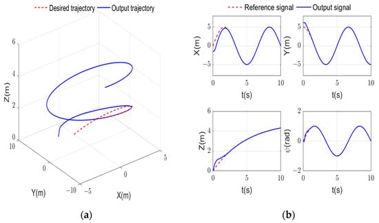
Figure 3. Tracking results. (a) 3D tracking curve; (b) tracking curves.

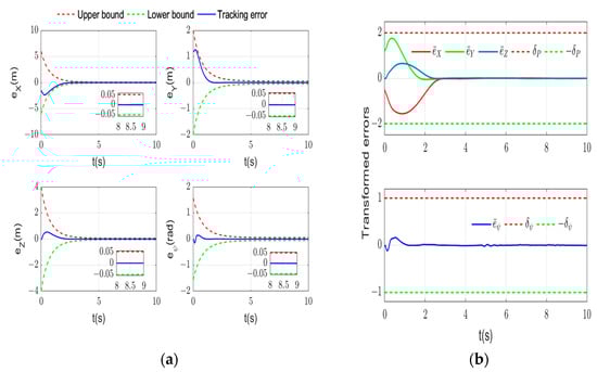
Figure 4. Tracking errors. (a) Tracking errors with the prescribed performance; (b) transformed errors.

The estimations of FTNNDO are respectively shown in Figure 5 and the estimation errors are shown in Figure 6, indicating that FTNNDO can deal well with unknown uncertainties, disturbances and derivatives of virtual control. The designed adaptive law can also effectively estimate the upper bound of NN error, as shown in Figure 7.

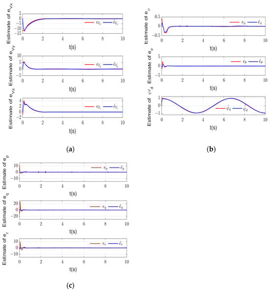
Figure 5. Estimations of FTNNDO. (a) Estimation of $e_V$; (b) estimation of $e_{\Theta }$; (c) estimation of $e_{\Omega }$.

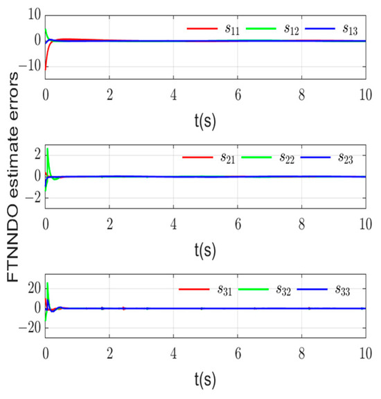
Figure 6. Estimation errors of FTNNDO.

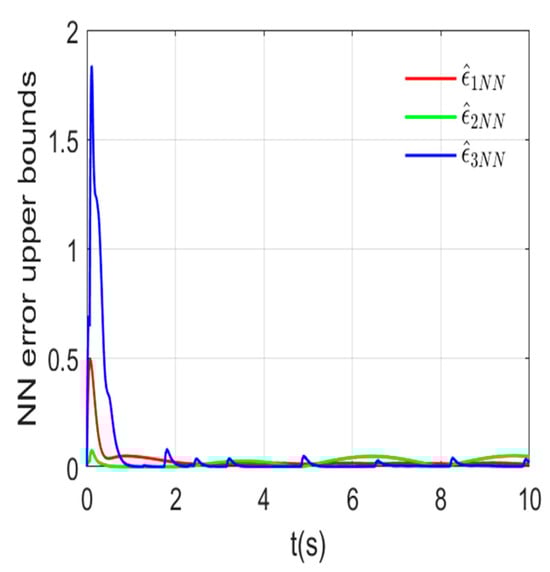
Figure 7. Estimations of NN error upper bounds.

The system states and control inputs are given in Figure 8 and Figure 9. It can be clearly observed that the all control inputs are chattering-free and bounded.

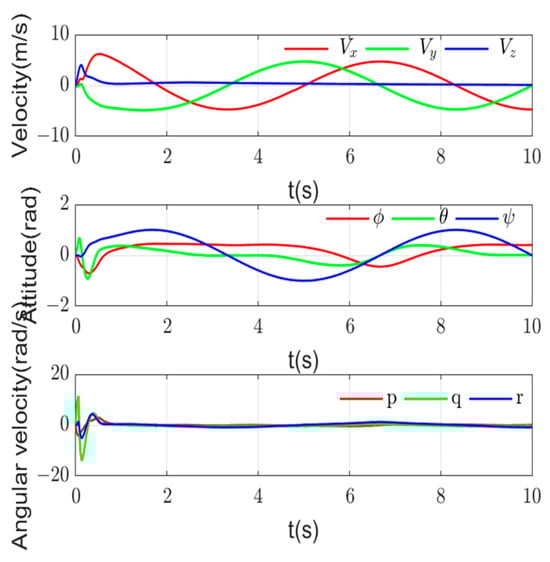
Figure 8. System states.

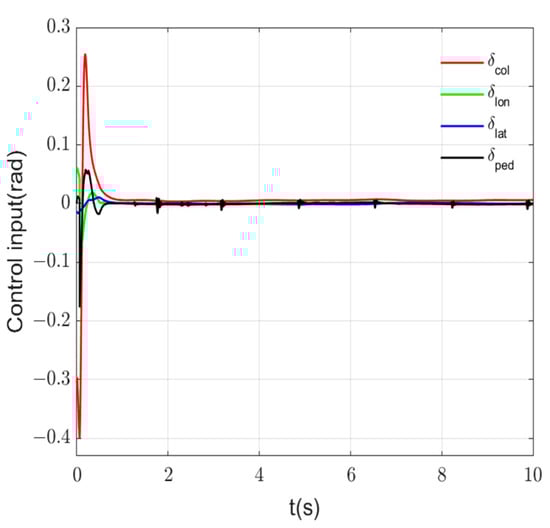
Figure 9. Control inputs.

In addition, to further demonstrate the superiority of the proposed method, two simulation tests are developed to compare the proposed method with existing ones.

• Test 1: Comparative simulation of the different prescribed performance methods

The tracking errors under the novel prescribed performance method in this paper (noted as M1) and the original one in [19,23] (noted as M2) are shown in Figure 10. It can be seen that the original method needs to set the different prescribed boundaries according to the different initial errors, while the method proposed in this paper can relax the requirement of initial errors, including initial symbols and values. The convergence time of position tracking error under the proposed method is less than 3.5 s, and the steady-state error accuracy is less than 0.01, while the convergence time under the original method is more than 5 s and the maximum steady-state error is about 0.04. Therefore, the proposed prescribed method can further improve the tracking performance.

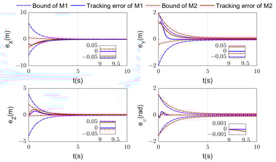
Figure 10. Tracking errors using different prescribed methods.

• Test 2: Comparative simulation of the different observer-based controllers

The DSC controller with an NDO observer (DSC-NDO) in [29], the BLF-based controller with a neural network observer (BLFC-NNDO) in [34] and the finite-time controller with a multivariable neural network observer (FTC-MNNDO) in [32] are compared with the proposed controller. The estimation results of observers are shown in Figure 11 and Figure 12. It can be seen that the proposed FTNNDO has a faster convergence rate and higher estimation accuracy than the other two observers. Meanwhile, by using the continuous hyperbolic tangent function with an adaptive gain to replace the fixed-gain sign function in [30,32,33], the estimation results under the FTNNDO are also chattering-free. The 3D tracking results and the tracking errors are shown in Figure 13. The convergence time of the proposed control method is about 3.5 s, and that of the FTC-MNNDO method is about 5.5 s, while the convergence speed of the other two asymptotic convergence methods are significantly slower. Moreover, the tracking accuracy of the proposed controller is also better than those compared schemes. Therefore, based on the FTNNDO and finite-time control laws, the control scheme proposed in this paper has more superiority.

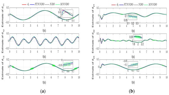
Figure 11. Observation curves. (a) Estimate of $d_1$; (b) estimate of $d_2$.

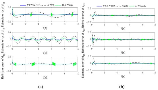
Figure 12. Estimate errors. (a) Estimate error of $d_1$; (b) estimate error of $d_2$.

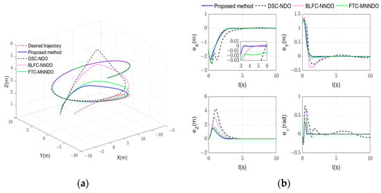
Figure 13. Tracking results. (a) 3D tracking curves; (b) tracking errors.

5. Conclusions

In this paper, an improved finite-time tracking controller is investigated for the UH system with performance constraints, model uncertainties and external perturbations. A novel prescribed performance function is designed to preset the tracking errors within prescribed boundaries, so that the transient tracking performance and steady-state accuracy can be reasonably constrained. A novel FTNNDO is proposed, which can quickly estimate the external disturbances and model uncertainties in finite time, as well eliminate the complicated differential calculation in the traditional backstepping design. Meanwhile, a continuous adaptive law is designed to dynamically tackle the NN approximate errors with unknown bounds and compensate online to improve the system robustness. Combining the novel prescribed performance function and FTNNDO, an improved tracking control controller with global finite-time convergence is developed. The stability of the proposed method is proven by introducing the BLF. All the closed-loop system signals and states are stable and bounded despite the model uncertainties and external disturbances. Compared with the existing control schemes, the proposed method has better tracking performance and robustness in finite time. The simulation results have demonstrated the effectiveness of the proposed control scheme. It is worth noting that the proposed control scheme is based on the assumption that all system states are measurable. Therefore, the future study needs to consider the unknown state under sensor failure. Meanwhile, actuator saturation can be further considered to enhance algorithm applicability.

References

- Yan, K.; Chen, M.; Wu, Q.; Zhu, R. Robust adaptive compensation control for unmanned autonomous helicopter with input saturation and actuator faults. Chin. J. Aeronaut. 2019, 32, 2299–2310. [Google Scholar] [CrossRef]
- Zhu, Y.; Xu, N.; Chen, X.; Zheng, W.X. H∞ control for continuous-time Markov jump nonlinear systems with piecewise-affine approximation. Automatica 2022, 141, 110300. [Google Scholar] [CrossRef]
- Shekhar, R.C.; Kearney, M.; Shames, I. Robust model predictive control of unmanned aerial vehicles using waysets. J. Guid. Control Dyn. 2015, 38, 1898–1907. [Google Scholar] [CrossRef]
- Fang, X.; Wu, A.; Shang, Y.; Dong, N. A novel sliding mode controller for small-scale unmanned helicopters with mismatched disturbance. Nonlinear Dyn. 2016, 83, 1053–1068. [Google Scholar] [CrossRef]
- Lai, Y.C.; Le, T.Q. Adaptive learning-based observer with dynamic inversion for the autonomous flight of an unmanned helicopter. IEEE Trans. Aerosp. Electron. Syst. 2021, 57, 1803–1814. [Google Scholar] [CrossRef]
- Gül, A.; Cakmak, E.; Karakas, A. Drone selection for forest surveillance and fire detection using interval valued neutrosophic edas method. Facta Univ.-Ser. Mech. Eng. 2024. online first. [Google Scholar] [CrossRef]
- Yang, J.H.; Hsu, W.C. Adaptive backstepping control for electrically driven unmanned helicopter. Control Eng. Pract. 2009, 17, 903–913. [Google Scholar] [CrossRef]
- Zhu, B.; Huo, W. Robust nonlinear control for a model-scaled helicopter with parameter uncertainties. Nonlinear Dyn. 2013, 73, 1139–1154. [Google Scholar] [CrossRef]
- Zhu, Y.; Wang, Z.; Liang, H.; Ahn, C.K. Neural-network-based predefined-time adaptive consensus in nonlinear multi-agent systems with switching topologies. IEEE Trans. Neural Netw. Learn. Syst. 2023, 35, 9995–10005. [Google Scholar] [CrossRef]
- Huang, Y.; Liu, W.; Li, B.; Yang, Y.; Xiao, B. Finite-time formation tracking control with collision avoidance for quadrotor UAVs. J. Franklin Inst. 2020, 357, 4034–4058. [Google Scholar] [CrossRef]
- Cao, Y.; Ren, W.; Meng, Z. Decentralized finite-time sliding mode estimators and their applications in decentralized finite-time formation tracking. Syst. Control Lett. 2010, 59, 522–529. [Google Scholar] [CrossRef]
- Zhao, L.; Jia, Y. Finite-time attitude tracking control for a rigid spacecraft using time-varying terminal sliding mode techniques. Int. J. Control 2015, 88, 1150–1162. [Google Scholar] [CrossRef]
- Bribiesca-Argomedo, F.; Krstic, M. Backstepping-forwarding control and observation for hyperbolic PDEs with Fredholm integrals. IEEE Trans. Autom. Control 2015, 60, 2145–2160. [Google Scholar] [CrossRef]
- Reddy, P.M.; Shimjith, S.R.; Tiwari, A.P.; Kar, S. Backstepping based model reference adaptive control for nuclear reactor with matched and unmatched uncertainties. Prog. Nucl. Energy 2023, 158, 104585. [Google Scholar] [CrossRef]
- Swaroop, D.; Hedrick, J.K.; Yip, P.P.; Gerdes, J.C. Dynamic surface control for a class of nonlinear systems. IEEE Trans. Autom. Control 2000, 45, 1893–1899. [Google Scholar] [CrossRef]
- Farrell, J.A.; Polycarpou, M.; Sharma, M.; Dong, W. Command filtered backstepping. IEEE Trans. Autom. Control 2009, 54, 1391–1395. [Google Scholar] [CrossRef]
- Yu, J.; Shi, P.; Zhao, L. Finite-time command filtered backstepping control for a class of nonlinear systems. Automatica 2018, 92, 173–180. [Google Scholar] [CrossRef]
- Zhao, Y.; Zhao, J.; Fu, J.; Shi, Y.; Chen, C. Rate bumpless transfer control for switched linear systems with stability and its application to aero-engine control design. IEEE Trans. Ind. Electron. 2020, 67, 4900–4910. [Google Scholar] [CrossRef]
- Bu, X. Guaranteeing prescribed output tracking performance for air-breathing hypersonic vehicles via non-affine back-stepping control design. Nonlinear Dyn. 2018, 91, 525–538. [Google Scholar] [CrossRef]
- Li, R.; Chen, M.; Wu, Q. Adaptive neural tracking control for uncertain nonlinear systems with input and output constraints using disturbance observer. Neurocomputing 2017, 235, 27–37. [Google Scholar] [CrossRef]
- Tee, K.P.; Ge, S.S.; Tay, E.H. Barrier Lyapunov functions for the control of output-constrained nonlinear systems. Automatica 2009, 45, 918–927. [Google Scholar] [CrossRef]
- He, W.; David, A.O.; Yin, Z.; Sun, C. Neural network control of a robotic manipulator with input deadzone and output constraint. IEEE Trans. Syst. Man Cybern. Syst. 2016, 46, 759–770. [Google Scholar] [CrossRef]
- Bechlioulis, C.P.; Rovithakis, G.A. Prescribed performance adaptive control for multi-input multi-output affine in the control nonlinear systems. IEEE Trans. Autom. Control 2010, 55, 1220–1226. [Google Scholar] [CrossRef]
- Han, S.I.; Lee, J.M. Improved prescribed performance constraint control for a strict feedback non-linear dynamic system. IET Control. Theory Appl. 2013, 7, 1818–1827. [Google Scholar] [CrossRef]
- Bechlioulis, C.P.; Rovithakis, G.A. Robust adaptive control of feedback linearizable MIMO nonlinear systems with prescribed performance. IEEE Trans. Autom. Control 2008, 53, 2090–2099. [Google Scholar] [CrossRef]
- Bechlioulis, C.P.; Doulgeri, Z.; Rovithakis, G.A. Neuro-adaptive force/position control with prescribed performance and guaranteed contact maintenance. IEEE Trans. Neural Netw. 2010, 21, 1857–1868. [Google Scholar] [CrossRef] [PubMed]
- Yu, J.; Shi, P.; Dong, W.; Yu, H. Observer and command-filter-based adaptive fuzzy output feedback control of uncertain nonlinear systems. IEEE Trans. Ind. Electron. 2015, 62, 5962–5970. [Google Scholar] [CrossRef]
- Chen, M.; Tao, G.; Jiang, B. Dynamic surface control using neural networks for a class of uncertain nonlinear systems with input saturation. IEEE Trans. Neural Netw. Learn. Syst. 2015, 26, 2086–2097. [Google Scholar] [CrossRef]
- Xu, B. Disturbance observer-based dynamic surface control of transport aircraft with continuous heavy cargo airdrop. IEEE Trans. Syst. Man Cybern. Syst. 2017, 47, 161–170. [Google Scholar] [CrossRef]
- Chen, L.; Zhu, Y.; Ahn, C.K. Adaptive neural network-based observer design for switched systems with quantized measurements. IEEE Trans. Neural Netw. Learn. Syst. 2023, 34, 5897–5910. [Google Scholar] [CrossRef]
- Chen, W.H.; Yang, J.; Guo, L.; Li, S. Disturbance-observer-based control and related methods—An overview. IEEE Trans. Ind. Electron. 2016, 63, 1083–1095. [Google Scholar] [CrossRef]
- Sun, H.; Guo, L. Neural network-based DOBC for a class of nonlinear systems with unmatched disturbances. IEEE Trans. Neural Netw. Learn. Syst. 2017, 28, 482–489. [Google Scholar] [CrossRef]
- Wang, D.; Zong, Q.; Tian, B.; Shao, S.; Zhang, X.; Zhao, X. Neural network disturbance observer-based distributed finite-time formation tracking control for multiple unmanned helicopters. ISA Trans. 2018, 73, 208–226. [Google Scholar] [CrossRef] [PubMed]
- Wang, X.; Wang, Q.; Sun, C. Adaptive tracking control of high-order MIMO nonlinear systems with prescribed performance. Front. Inform. Technol. Electron. 2021, 22, 986–1001. [Google Scholar] [CrossRef]
- Qian, C.; Lin, W. A continuous feedback approach to global strong stabilization of nonlinear systems. IEEE Trans. Autom. Control 2001, 46, 1061–1079. [Google Scholar] [CrossRef]
- Tong, S.; Sui, S.; Li, Y. Fuzzy adaptive output feedback control of MIMO nonlinear systems with partial tracking errors constrained. IEEE Trans. Fuzzy Syst. 2015, 23, 729–742. [Google Scholar] [CrossRef]
Disclaimer/Publisher’s Note: The statements, opinions and data contained in all publications are solely those of the individual author(s) and contributor(s) and not of MDPI and/or the editor(s). MDPI and/or the editor(s) disclaim responsibility for any injury to people or property resulting from any ideas, methods, instructions or products referred to in the content. |
© 2024 by the authors. Licensee MDPI, Basel, Switzerland. This article is an open access article distributed under the terms and conditions of the Creative Commons Attribution (CC BY) license (https://creativecommons.org/licenses/by/4.0/).