Classification Model for Real-Time Monitoring of Machining Status of Turned Workpieces

Abstract

The occurrence of tool chatter can have a detrimental impact on the quality of the workpiece. In order to improve surface quality, machining stability, and reduce tool wear cycles, it is essential to monitor the workpiece machining process in real time during the turning process. This paper presents a tool chatter state recognition model based on a denoising autoencoder (DAE) for feature dimensionality reduction and a bidirectional long short-term memory (BiLSTM) network. This study examines the feature dimensionality reduction method of the DAE, whereby the reduced-dimensional data are concatenated and input into the BiLSTM model for training. This approach reduces the learning difficulty of the network and enhances its anti-interference capability. Turning experiments were conducted on a SK50P lathe to collect the dataset for model performance validation. The experimental results and analysis indicate that the proposed DAE-BiLSTM model outperforms other models in terms of prediction and classification accuracy in distinguishing between stable machining, over-machining, and severe chatter stages in turning chatter state recognition. The overall classification accuracy reached 96.28%.

1. Introduction

The machining stages of the workpiece can be divided into three categories according to the form of the vibration signal: stable machining, excessive machining, and severe chattering. The occurrence of tool chatter can have a detrimental impact on the quality of the workpiece [1]. It is estimated that over 75% of machine failures are attributable to severe tool wear or malfunction. From an economic perspective, the cost of maintaining the condition of the tool and replacing it when necessary represents a significant proportion of the overall production costs, with estimates ranging from 3% to 12% [2]. Approximately 20% of the downtime is attributable to tool failure, whereby the tool gradually wears during the cutting process, resulting in irreversible damage to the workpiece and potentially catastrophic tool failure [3]. Consequently, the development of a tool chatter state identification system is required in order to effectively predict the machining state of the tool, optimize the tool life, improve the quality of the workpiece, and reduce the degree of tool wear.

The turning process is a widely used machining method in contemporary mechanical manufacturing. The reduction of workpiece deformation, the improvement of surface quality, and the enhancement of turning efficiency represent ongoing research hotspots in the field of turning process optimization [4]. The stability of the machining process has a significant impact on the quality and efficiency of turning operations [5]. The intense chatter generated by the cutting tool during the machining of the workpiece not only has a substantial negative impact on the surface accuracy of the machined workpiece but also severely compromises the lifespan of the machining equipment and the safety of the production process. Research on chatter monitoring and prevention addresses this critical issue, which has significant scientific research value [6]. Therefore, to improve the quality of the turning process, it is essential to conduct an in-depth study on process state monitoring and recognition.

In previous studies, researchers employed machine learning methodologies to model the relationship between tool flutter recognition and sensor signals. For example, support vector machines (SVMs) [7] and hidden Markov models (HMMs) [8] were utilized. Gao and Liao et al. [9] proposed a multi-scale statistical signal processing method based on a wavelet domain hidden Markov tree and a hybrid hidden Markov model for monitoring the wear state of turning tools. However, the accuracy and reliability of this model in identifying signal features during the transitional processing stage are deemed insufficient.

In contrast to the aforementioned research methods, neural networks have demonstrated outstanding performance in pattern recognition and feature classification. This is attributed to their internal node weight mechanisms. Neural networks learn by identifying and correcting discrepancies between predicted and actual outcomes [10]. Notable examples include convolutional neural networks (CNNs) [11], artificial neural networks (ANNs) [12,13], and long short-term memory networks (LSTMs) [14,15]. Some scholars have applied a time–frequency image of the force signal to a CNN model [16] by combining an analytical solution and the CNN model under a new transfer learning framework [17]. However, unidirectional LSTMs may be susceptible to information loss when processing long time series data. Gang et al. [18] proposed a novel unified architecture that incorporates bidirectional LSTM (BiLSTM) [19], attention mechanisms, and convolutional layers. This architecture is designated as the attention-based convolutional layer bidirectional long short-term memory (AC-BiLSTM). The results demonstrate that AC-BiLSTM outperforms other advanced text classification methods in terms of classification accuracy. Yang et al. [20] proposed a periodic defect detection method that combines convolutional neural networks (CNNs) and long short-term memory (LSTM) networks. In this approach, the convolutional neural network (CNN) is employed to extract features from defect images, which are subsequently input into the long short-term memory (LSTM) network for defect recognition. An attention mechanism is introduced to enhance the detection rate. Although convolutional neural networks (CNNs) are highly effective at extracting image features, they are less efficient at handling time series signals. This is because they are unable to fully capture the temporal dependencies within the signals. Chen et al. [21] employed deep belief networks (DBNs) to monitor tool wear, conducting experiments on datasets comprising force, vibration, and acoustic emission signals from the milling process [22,23,24]. The results indicate that this model exhibits more stable prediction performance than support vector regression (SVR) and ANN. However, the absence of effective feature dimensionality reduction techniques may result in the introduction of superfluous information or the loss of crucial features, thereby affecting the model’s predictive capabilities.

In order to facilitate the subsequent recognition and classification processes, it is common practice to incorporate an autoencoder (AE) and a denoising autoencoder (DAE) [25]. The findings of Luo et al. [26] indicated that, when the number of features exceeds a certain threshold, their contribution to the performance becomes less pronounced. Therefore, an unsupervised method is proposed to enhance classification outcomes through in-depth research and the integration of multi-level classifiers with a limited number of features per layer. By employing the denoising autoencoder (DAE) to train the network in a layer-by-layer manner, the convolution kernel is optimized to enhance performance. Kuo et al. [27] employed t-distributed stochastic neighbor embedding (t-SNE) to reduce dimensionality while preserving the local data structure in the analysis of flutter signals. t-SNE effectively reduces the dimensionality of high-dimensional data, thereby decreasing the computational load following synchronous compression. Feature dimensionality reduction involves transforming the original high-dimensional data into a low-dimensional space while retaining the primary features and structure of the data. This process aims to enhance data interpretability and algorithm efficiency while minimizing computational costs and storage requirements.

To address these issues, this paper proposes a DAE-BiLSTM model for tool chatter state recognition. The denoising autoencoder (DAE) is employed to perform feature dimensionality reduction on the signals collected by triaxial acceleration sensors. This process reduces redundant information while retaining critical information, thereby enhancing the feature extraction accuracy. Subsequently, the bidirectional long short-term memory (BiLSTM) network is employed to train the dimensionally reduced signals, effectively capturing the temporal dependencies within the signals and mitigating information loss. By processing sequence data bidirectionally, the BiLSTM enhances the model’s performance in handling long time series data. Consequently, this model ultimately enhances the accuracy of tool chatter state recognition during the turning process.

Compared to other studies under similar working conditions, the recognition method designed in this paper offers several advantages: (1) The combination of DAE and BiLSTM is relatively novel. By leveraging the characteristics of turning chatter signals over time, the BiLSTM model is utilized for flutter classification, and DAE is introduced to reduce the training difficulty of neural networks and improve the classification accuracy of the flutter state recognition model. (2) There is limited research on the specific working conditions addressed in this paper. The combination of DAE and BiLSTM algorithms achieves an overall recognition accuracy of 96.28%, which is highly effective for the working conditions discussed.

2. Turning Stability Prediction Theory Analysis

Regenerative chatter represents the principal form of turning chatter. The generation and development of chatter can have a significant impact on the quality of the machined workpieces and the safety of the equipment used in the process. In order to ensure the stability of the turning process, it is necessary to study the prediction of stability during the machining process and the use of online monitoring methods. The criteria for evaluating stability are established, and the stages of chatter development are classified according to changes in the workpiece surface quality over time. A turning chatter dynamics model was constructed, and a turning stability domain leaflet diagram was generated [28,29].

2.1. Establishment of Evaluation Criteria for Turning Stability

The purpose of establishing the turning stability evaluation standard is to select the appropriate workpiece surface. The quality of the workpiece surface directly influences chatter during processing. At present, surface evaluation standards include a geometric error, surface waviness, and surface roughness. This paper will establish the evaluation standard of turning stability by measuring the surface roughness of the workpiece and observing the surface quality of the workpiece.

In cylindrical turning, the surface roughness of the workpiece is recorded when the cutting length is 100 mm, as shown in Table 1. Combined with the data in the table, the processing can be divided into the following three stages: when Ra < 3.2 μm, the workpiece surface is free of vibration marks, and machining is in the stable processing stage; when 3.2 μm < Ra < 12.5 μm, the vibration mark on the workpiece surface is not obvious, and machining is in the over-machining stage; and when Ra > 12.5 μm, the surface of the workpiece has obvious chatter marks, and machining is in the chattering stage.

Table 1. Surface roughness values of cylindrical turning.

Distance from start (mm)	5	10	15	20	25	30
Surface roughness Ra (μm)	2.17	2.12	2.10	2.11	2.32	2.55
Distance from start (mm)	35	40	45	50	55	60
Surface roughness Ra (μm)	5.80	15.26	16.23	16.17	15.11	16.22
Distance from start (mm)	65	70	75	80	85	90
Surface roughness Ra (μm)	15.44	17.32	15.31	15.32	16.30	15.21

2.2. Turning Chatter Dynamics Modeling

In order to study the stability of turning and more accurately identify the turning chatter state, it is necessary to employ a methodology that allows for the examination of the aforementioned phenomena in a controlled environment. Prior to the commencement of machining, it is necessary to establish the dynamics model of the machine tool–tool–workpiece system. The weak link of tool stiffness of the horizontal lathe used in the test frequently manifests in the feed direction Z and the main cutting Y direction perpendicular to the base surface. Consequently, the machining system can be simplified to a two-degrees-of-freedom system, as illustrated in Figure 1a, and the corresponding transfer function is depicted in Figure 1b. In accordance with the established definition of dynamic cutting thickness, the following kinetic Equation (1) can be formulated.

$$m\ddot{z}(t)+c_z\dot{z}(t)+k_{z}z(t)={(K_p+K_q)}_z{a}_p\left[z(t-T)-z(t)\right]$$

(1)

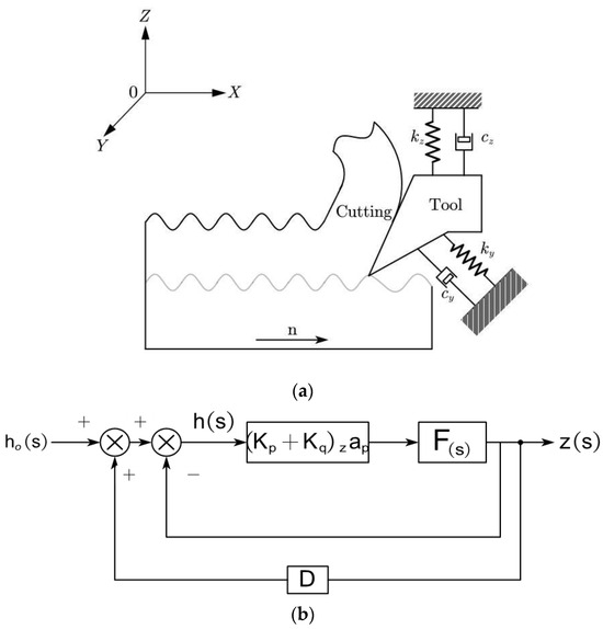
Figure 1. Machining system dynamics model. (a) Machining system dynamics diagram. (b) System transfer function.

In Equation (1), $z(t)$ is the cutting period in the Z direction; $m$, $c_z$, and $k_z$ are the modal mass, damping, and stiffness in the Z direction; $k_p$ is the cutting force coefficient in the parallel direction of the front tool face; $k_q$ is the cutting force coefficient in the vertical direction of the front tool face; and $a_p$ is the unilateral depth of the cut in mm.

2.3. Turning Stability Domain Leaflet Diagram Solution

The system modal parameters and transfer functions were employed to generate the SLD diagram depicted in Figure 2, which depicts the limited cutting depth corresponding to the turning and tool in the spindle speed range of 400~1600 rpm. The horizontal coordinate of the SLD diagram is the spindle speed $\mathrm{n}$ in rpm, while the vertical coordinate is the limited cutting depth corresponding to the speed $\mathrm{apm}$ in mm.

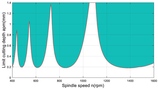
Figure 2. Cutting stable domain leaflet diagram.

The flap-shaped curve formed by the limited cutting depth represents the theoretical stability boundary of the machining system. Under the theoretical conditions, selecting the process parameters in the white area below the curve can avoid chatter, and the machining process will be stable; selecting the process parameters in the dark area above the curve boundary will excite chatter, and the machining process will have violent vibrations; and selecting the process parameters near the boundary will put the machining system in the transition machining state. Thus, a prediction model based on deep learning is designed, and the chatter signals are collected experimentally, denoised, and put into the prediction model for learning training to verify that the model makes more accurate classification at each stage.

3. Research Methods and Predictive Models

3.1. DAE

The vibration signal samples collected by the test in this paper include acceleration vibration signals in three directions, which inevitably include the fusion of complex feature information from three dimensions. The direct introduction of multi-dimensional complex sample information into the prediction model for training will lead to huge training tasks, a long training time, and even lead to non-convergence of the network. Therefore, it is necessary to reduce the dimension of the original input signal to reduce the complexity of the input samples while retaining the key signal features.

DAEs are enhanced versions of autoencoders [30]. Common types of autoencoders include stacked autoencoder, undercomplete autoencoder, regular autoencoder, and denoising autoencoder. It is challenging for the autoencoder to extract more useful features based solely on the reconstruction criterion. Therefore, the reconstruction criterion is modified to denoising; in other words, destructive noise interference signals are added to the input layer, causing partial loss of the original data values from the input sequence [31]. The training network then restores the original samples of unlost data, and the learned signal is utilized as the input throughout training. This allows for a more objective evaluation of its usefulness and enhances the robustness of the output features. The structure of the DAE network is depicted in Figure 3.

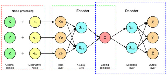
Figure 3. DAE network structure.

In the training process of the DAE network, firstly, the elements in the acceleration signal in the three directions of the input matrix $I=\{X,Y,Z\}$ are removed according to a certain proportion $q_D$, and the matrix $Ie=\{Xe,Ye,Ze\}$ containing the noise sequence is obtained, then connected to two coding layer neurons $S_{E1},S_{E2}$ to obtain the abstract features x after completing the coding process, and the expression form of the coding process function is shown in Equation (2).

$$C=f(W_{E}x+b_E)$$

(2)

In Equation (2), $f$ is the encoding function, $W_E$ is a $d^{\prime }\times d$ weight matrix, and $b_E$ is an offset vector of dimension $d^{\prime }$. The abstract feature $C$ has a minimum number of neuron nodes after encoding is completed, and in this paper, the three-dimensional input is compressed into one dimension, i.e., the abstract feature $C$ has only one neuron node. The abstract feature $C$ continues to be connected to two coding layer neurons $S_{D1},S_{D2}$, and the final output is the decoded reconstructed matrix $y=\left\{\overline{X,}\overline{Y,}\overline{Z}\right\}$. The mathematical expression of the decoding process is shown in Equation (3).

$$y=g(W_{D}C+b_D)$$

(3)

In Equation (3), $g$ is the decoding function, $W_E$ is a $d^{\prime }\times d$ weight matrix, and $b_E$ is an offset vector of dimension $d^{\prime }$. The denoising autoencoder considers the decoding reconstruction error as the network loss value and minimizes the loss as the network training goal. Define the network input $I=\{X,Y,Z\}$, output $O=\left\{\overline{X,}\overline{Y,}\overline{Z}\right\}$, sequence length $n$, and loss value $L_D$ as shown in Equation (4).

$$L_D={\displaystyle \sum _{i=1}^n-O_i\ln \left(I_i\right)}$$

(4)

When $L_D$ converges to the satisfactory interval, the training of the denoising autoencoder is completed, the encoder part is intercepted as the feature downscaling preprocessing network, and the downscaled abstract features $C$ are used as the network output. The iterative training $L_D$ descends to a satisfactory interval.

3.2. BiLSTM

In the traditional neural network model, signal transmission is based on the signal before time t for the judgment prediction. In order to make sure the predicted information contains the before and after time, two LSTM networks are used to predict the signal from the forward and reverse directions, respectively, to improve the accuracy. In the process of turning machining, the excitation process of chattering always moves from the stable machining stage to the transition machining stage, eventually developing into severe chattering, with a more fixed sequence. Based on this characteristic, if the input signals of previous and future moments are integrated for training in the LSTM network model construction, the accuracy of the model recognition can be improved in theory. The unidirectional LSTM network can only predict the output of the current moment based on the previous moment information, and in order to achieve data processing in both directions, a BiLSTM [32,33,34] structure as shown in Figure 4 needs to be used.

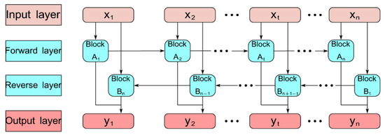
Figure 4. BiLSTM network structure.

BiLSTM adds a set of blocks with the opposite transfer direction to the hidden layer of normal LSTM, called the reverse layer, and the original blocks are called the forward layer. The forward layer has the same transfer direction as time and is responsible for processing the input data of the previous moment, while the reverse layer has the opposite transfer direction as time and is responsible for processing the input data of the future moment. The forward and reverse layers are jointly connected to the output layer, so the output expression for any moment $t$ is shown in Equation (5).

$$y_t=\mathrm{Softmax}\left(W_A{H}_{At}+W_B{H}_{Bn+1-t}+b\right)$$

(5)

In Equation (5), $H_{At}$ and $H_{Bn+1-t}$ are the hidden element outputs of the forward and reverse layers at moment $t$, respectively, $W_A$ and $W_B$ are the forward and reverse layer weights, respectively, and $b$ is the output layer bias.

3.3. DAE-BiLSTM Tool Chatter Prediction Model

A flow chart of the DAE-BiLSTM-based tool chatter prediction model is constructed from above. As shown in Figure 5, the cutting signals are collected experimentally, and the surface quality is evaluated. The model consists of two parts: DAE is responsible for the input of the vibration signal, normalization, and feature dimensionality reduction, and the BiLSTM network is responsible for training the encoded one-dimensional abstract features for state recognition. Finally, the evaluation results and model training results are combined to identify and classify the chatter states.

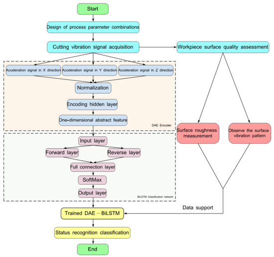
Figure 5. Flutter state identification flow chart based on the DAE-BiLSTM model.

4. Experiment Design and Network Model Training

4.1. Experimental Flow Design

The turning chatter experiment in this paper is mainly responsible for collecting the vibration signals during machining, analyzing, and denoising them. In this paper, the SK50P machine tool is taken as the experiment object to carry out the cylindrical cutting experiment on the workpiece, and the performance parameters are shown in Table 2. In this experiment, the workpiece utilized is 20MnCrS5 carburized steel, featuring a diameter of φ50 mm and a length of 500 mm. Table 3 lists the chemical components, and Table 4 lists the main performance. The tool is made of a 93-degree triangular outer lathe tool bar and TNMG160404R-S metal ceramic blades. Table 5 lists its physical characteristics. Figure 6 showcases both the workpiece and the cutting tool.

Table 2. The SK50P machine performance parameters.

Spindle Speed (r/min)	Machining Accuracy (Ra)	Maximum Cutting Diameter (mm)	Maximum Cutting Length (mm)	Two-Axis Travel (mm)
21~1620	1.6	500	820	X: 300 Z: 850

Table 3. The 20MnCrS5 chemical composition (mass fraction/%).

Designation	C	Si	Mn	Cr	S	P
20MnCrTi	0.17~0.23	0.17~0.37	1.10~1.40	0.80~1.10	0.02~0.04	≤0.025

Table 4. The 20MnCrS5 main performance.

Designation	Tensile Strength /(Mpa)	Yield Strength /(Mpa)	Elongation /(%)	Section Shrinkage /(%)	Impact Work /(J)	Impact Toughness /(J/cm2)	Hardness /(HRC)
20MnCrTi	≥1000	≥600	≥10	≥40	≥40	≥50	55

Table 5. Physical properties of the TNMG160404R-S tool.

Designation	Young’s Modulus /(Gpa)	Thermal Conductivity/(W/m·K)	Poisson’s Ratio	Density /(g/cm3)	Specific Heat /(J/kg·°C)
TNMG160404R-S	420	30	0.25	5.5	450

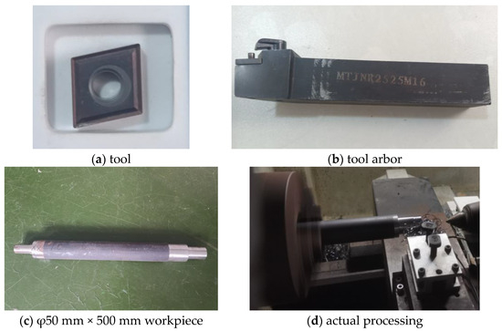
Figure 6. The TNMG160404R-S tool and 20MnCrS5 workpiece.

Therefore, a chattering signal monitoring system is composed of a CNC machine, sensor, data acquisition card, and computer, as shown in Figure 7.

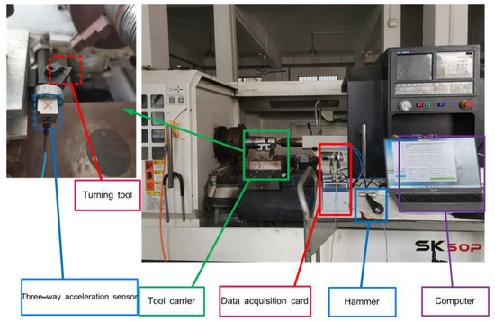
Figure 7. Machine tool test platform.

The experimental process of turning vibration machining includes three main steps: process parameter combination design, cutting vibration signal acquisition, and workpiece surface quality evaluation. Formulate the combination of the cylindrical turning process parameters, as shown in Table 6. The design of the process parameter combination in the experiment was studied from three aspects: rotational speed, feeds, and unilateral depth of cut. Three sets of rotational speeds (600 r/min, 800 r/min, and 1000 r/min); three sets of feeds (F50, F100, and F150); and nine sets of unilateral depths of cuts in each set of rotational speeds were used for a total of 81 tests. The build monitoring system was used to collect the acceleration vibration signals in three directions during the processing and preliminarily analyze the signal samples. After the workpiece is processed, the TR210 handheld surface roughness measuring instrument was used to measure the surface roughness of the machined surface. The acceleration signals and surface roughness were recorded for each set of process parameters.

Table 6. Combination of cutting test process parameters.

Group	Spindle Speed (r/min)	Cutting Depth (mm)	Theoretical State	Feed Rate (mm/min)
1	600	0.10, 0.15, 0.20	stable	F50, F100, F150
2		0.25, 0.30, 0.35	transition
3		0.40, 0.45, 0.50	severe
4	800	0.10, 0.15, 0.20	stable	F50, F100, F150
5		0.25, 0.30, 0.35	transition
6		0.40, 0.50, 0.55	severe
7	1000	0.40, 0.45, 0.50	stable	F50, F100, F150
8		0.55, 0.60, 0.65	transition
9		0.70, 0.75, 0.80	severe

To implement the DAE denoising algorithm and the DAE-BILSTM flutter classification model in the actual turning process, this study has designed a turning flutter monitoring software incorporating the aforementioned algorithms. The software is developed using MATLAB2022a’s integrated APP design tool, enabling the direct invocation of algorithms, networks, and models that are programmed and trained within the MATLAB environment. The software integrates functionalities for signal acquisition, signal analysis and preprocessing, flutter recognition, and data management, all presented through an intuitive user interface.

4.2. Analysis of the Test Results

According to the process parameter combination given in Table 6, the cylindrical cutting test of the 20MnCrS5 bar is carried out to obtain the stable, transition, and flutter vibration signals at different speeds. Table 7 shows the three machining conditions observed at 600 r/min speed, feed F50, and different depths of cuts. This provides detailed data support for the next step of model learning training. Figure 8 intercepts some time–frequency waveforms of acceleration signals in the Z direction corresponding to them and takes this as an example for analysis.

Table 7. Comparison of the surface morphology and roughness under different processing conditions.

	State	Stable Processing	Transition Processing	Severe Tremors
Indicators
Surface appearance
Process parameters		S600, F50, ap = 0.10 mm	S600, F50, ap = 0.30 mm	S600, F50, ap = 0.50 mm
Ra value (μm)		2.551	4.737	18.628

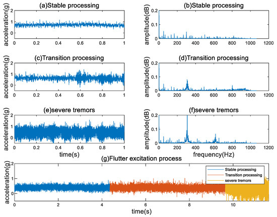
Figure 8. Time–frequency waveform of the Z direction acceleration under three processing conditions.

When the single side cutting depth is 0.1 mm, the whole turning process is stable without abnormal noise, and the time domain waveform of the acceleration signal is linear and uniform, as shown in Figure 8b. When the single side cutting depth is 0.3 mm, there is no obvious abnormal noise during the turning process. The time domain waveform of the acceleration signal is similar to that in the stable phase, but an instantaneous unstable jitter will occur randomly, as shown in Figure 8c. At the same time, the trend of the energy concentration appears on the spectrum, as shown in Figure 8d. When the unilateral cutting depth is 0.5 mm, significant abnormal vibrations start to appear in the turning process, as shown in Figure 8e, corresponding to the amplitude of the acceleration signal shown in Figure 8f increasing and continuing to shake, and significant peaks appear in the spectrum.

4.3. DAE Training Results

The DAE neural network constructed in this paper is sequentially connected with an input layer of dimension 3, a fully connected layer with dimensions 3–2–1–2–3, and a regression layer of dimension 3. According to the surface roughness measurement results, the test groups of the three processing stages can be selected, and the corresponding signals are divided into samples with an interval of 0.5 s. The vibration signal samples collected in this study contain acceleration vibration signals in three directions. However, the 3D signal features are complex, and directly introducing multi-dimensional complex sample information into the prediction model results in extensive training tasks, prolonged training times, and potential issues with network convergence. To address this, we reduce the dimensionality of the original input signal to one dimension, thereby decreasing the complexity of the input sample while preserving key signal features. Each sample is a 3 × 1066 matrix, including 1066 sampling points in three directions. The defective samples were deleted, and 3072 groups of samples were finally screened, including 1078 groups of samples in the stable processing stage, 931 groups of samples in the transitional processing stage, and 1063 groups of samples in the flutter stage. After noise reduction, these samples are divided into a training set, test set, and validation set according to 7:2:1. The training set is randomly corrupted with a 30% noise ratio. The network converges after 100 iterations. The loss values and RMSE decreases during the training process are observed as shown in Figure 9.

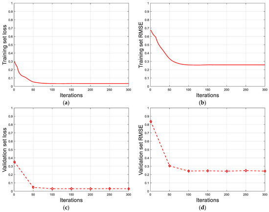
Figure 9. DAE network training results. (a) Training set loss value, final value: 0.0339. (b) Training set RMSE, final value: 0.2604. (c) Verification set loss value, final value: 0.0291. (d) Validation set RMSE, final value: 0.2411.

The RMSE index reflects the similarity between the denoised signal $\overline{F}\left(\mathrm{t}\right)$ and the original signal $F\left(t\right)$. The smaller the value is, the more complete the feature restoration of the denoised signal to the original signal is, and the better the denoising effect. The calculation method is shown in Equation (6).

$$RMSE=\sqrt{{\displaystyle \frac{1}{N}}{\displaystyle \sum _{t=1}^N{\left[F(t)-\overline{F}(t)\right]}^2}}$$

(6)

In addition, we used ANOVA (Analysis of Variance) to analyze the differences between the original signal and the reconstructed signal, thereby evaluating the effect of DAE processing. As shown in Figure 10, the median values of the original and reconstructed data are very similar, and the interquartile ranges are almost identical. The calculated p-value of 0.564 (p > 0.05) indicates that there is no significant difference between the original signal and the reconstructed signal. Therefore, the DAE performs well in signal reconstruction and is capable of retaining the features of the original signal.

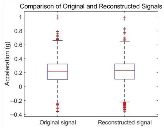
Figure 10. Comparison of the original and reconstructed signals.

Figure 11 shows the waveform comparison of the original sample, the sample after noise pollution, and the sample after reconstruction of a random sampling group of test set samples. Based on the average RMSE value of the test set at each processing stage, as shown in Table 8, the average RMSE value of the overall test set samples is 0.1075, which is consistent with the expectation of the convergence of the validation set during the training process.

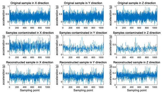
Figure 11. Comparison of sample waveforms before and after reconstruction.

Table 8. Evaluation results of the test set reconstruction samples.

Processing Stage	Stable Processing	Transition Processing	Severe Tremors	Overall Average
RMSE average	0.0672	0.1218	0.1335	0.1075

4.4. DAE-BiLSTM Model Training Results

Prior to training, the neural network requires the initialization of the parameters, known as hyperparameters. The hyperparameters that significantly impact the training performance of the BiLSTM network include batch size, number of training epochs, number of hidden units, learning rate, and gradient threshold. In this study, the hyperparameters were set as follows: the batch size was 43, the number of epochs was 22, the number of hidden units was 100, the learning rate was 0.01, and the gradient threshold was 1. The training set and corresponding labels are fed into the DAE-BiLSTM network with completed hyperparameter settings for training, and gradient descent optimization is performed using the Adam solver. Since the DAE has been pretrained and achieved the expected results, it is necessary to lock the weight parameters of the DAE part in advance and only update the parameters of the BiLSTM network. The network tends to converge after 500 iterations, and the accuracy and loss values during the learning process are collected, as shown in Figure 12.

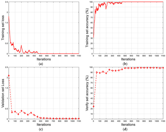
Figure 12. DAE-BiLSTM network training results. (a) Training set loss value, final value: 0.0184. (b) Training set accuracy, final value: 100%. (c) Verification set loss value, final value: 0.0655. (d) Verify set accuracy, final value: 96.14%.

5. Analysis and Discussion of the Classification Results

A total of 3072 groups of samples were selected for this experiment. The dataset was divided into a training set, test set, and validation set at a ratio of 7:2:1 to train the network. The test set completed by DAE training is fed into the DAE-BiLSTM model for training, and the prediction results are compared to the LSTM, BiLSTM, DAE-BiLSTM, and PCA-BiLSTM networks trained under the same configuration. The PCA-BILSTM model is a combination of PCA (principal component analysis) and BiLSTM. The confusion matrix of the error cases of the prediction results and the real results are shown in Figure 13.

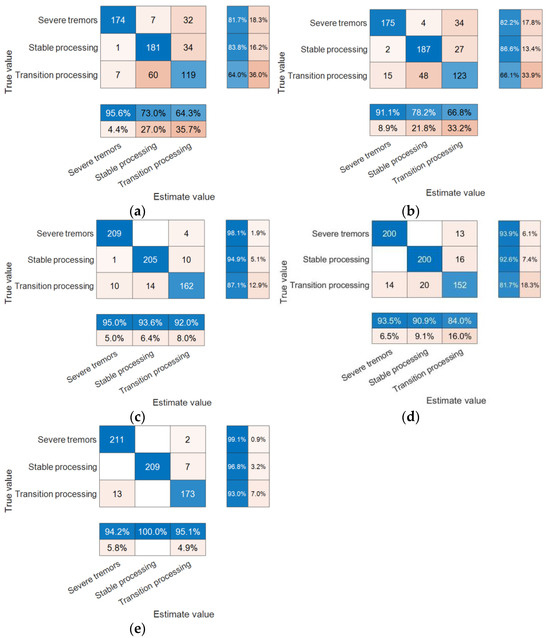
Figure 13. Classification results by network. (a) LSTM network. (b) BiLSTM network. (c) DAE-LSTM network. (d) PCA-BiLSTM network. (e) DAE-BiLSTM network.

Based on the results shown in Figure 13, the classification accuracy of the five networks for signals at different processing stages was calculated, and the results are shown in Table 9.

Table 9. Comparison of the classification accuracy of each network test set.

Serial Number	Network Model	Stable Processing	Transition Processing	Severe Tremors	Overall Accuracy
1	LSTM	83.80%	63.98%	81.69%	76.49%
2	BiLSTM	86.57%	66.13%	82.16%	78.29%
3	PCA-BiLSTM	92.58%	81.73%	93.87%	89.39%
4	DAE-LSTM	94.91%	87.10%	98.12%	93.38%
5	DAE-BiLSTM	96.76%	93.01%	99.06%	96.28%

(1)

The effect of introducing DAE on the chattering state recognition results: The comparisons of groups 1–4 and 2–5 show that the LSTM/BiLSTM network with the adding of the DAE feature reduction encoder has a more significant improvement in the classification of samples at different processing stages. The input samples after feature downscaling reduced the learning difficulty of the recognition network and improved the classification accuracy of all processing stages, and the final overall classification accuracy improved from 76.49% and 78.29% to 93.38% and 96.28%, respectively.

(2)

The effect of introducing BiLSTM on the chattering classification results: The comparisons of groups 1–2 and 4–5 show that changing the unidirectional LSTM network to a bidirectional LSTM network has a less significant contribution to the overall classification accuracy improvement, mainly improving the classification accuracy of the overprocessing stage, and finally, the classification accuracy of the transition processing stage improved from 63.98% and 87.10% to 66.13% and 93.01%, respectively. In addition, the comparison of group 3–5 shows that the overall accuracy of the DAE-BiLSTM was higher than that of the PCA-BiLSTM. This indicates that the combined effect of DAE and BiLSTM is superior to that of PCA and BiLSTM.

(3)

By comparing the classification accuracies of the four groups of different processing stages, it can be seen that the classification accuracy of each network for both the stable processing and the intense chattering stages are significantly higher than those for the transition processing stage. The transition processing stage has a short duration, few signal samples, and some characteristics of both stable processing and severe chattering, so the classification accuracy is lower than the other two stages.

In summary, the DAE-BiLSTM chattering state recognition model proposed in this paper can effectively identify the turning vibration signals of three machining states: stable machining, excessive machining, and severe chattering, with an overall classification accuracy of 96.28%. Compared to the original LSTM model, the DAE-BiLSTM model has a significantly improved performance. Therefore, it can be applied to the turning process and carry out the online recognition of chattering state during the machining process.

6. Conclusions

In this paper, the monitoring and prevention of tool chatter is explored through turning machining tests. Based on this, a tool chatter prediction model based on acceleration vibration signals is established by using a DAE-BiLSTM network, and the following conclusions are drawn by comparing and analyzing with the unoptimized LSTM network.

(1)

Through the dynamic modeling and the plotting of stable blade diagram, it is found that the different stages of turning need further online monitoring to avoid the damage of the workpiece and tool in turning.

(2)

The DAE-BiLSTM proposed in this paper can be trained to predict and classify tool chatter values with small-scale samples and successfully predict the trend of tool chatter and identify the current state of the workpiece.

(3)

By comparing the signal acquisition values at each stage, the proposed DAE-BiLSTM has more advantages in prediction and classification accuracy than the original LSTM network and improves the sensitivity of the LSTM network model in predicting the characteristics of tool chattering signals.

The algorithm developed in this paper has been applied to the actual production process at Dongfeng Motor Co., Ltd., demonstrating practical benefits for production improvement. By using our proposed DAE-BiLSTM model, Dongfeng Motor Co., Ltd. has achieved enhanced identification accuracy, enabling timely adjustment of the processing parameters. This results in reduced tool wear, lower replacement costs, shortened downtime due to tool failure, improved production efficiency, and better machining quality.

In summary, the turning chatter prediction model proposed in this paper has a high feasibility and provides a certain research basis for the signal monitoring of CNC machine tools. The present study has accomplished the model training using a single acceleration sensor signal. To enhance the model’s accuracy, future work may incorporate the use of multiple sensors to monitor the flutter states. It is suggested to further explore multi-sensor fusion technology to improve the significance and robustness of the target features. Additionally, to ensure the stability of the machining process and enable the chatter monitoring study to provide optimal decisions, closed-loop control strategies associated with the machining system should be investigated. Future research could focus on the automatic optimization of the process parameters by adjusting the speed and cutting depth, thereby preventing the excitation of turning chatter and achieving intelligent process planning.

References

- Shrivastava, Y.; Singh, B. Tool chatter prediction based on empirical mode decomposition and response surface methodology. Measurement 2021, 173, 108585. [Google Scholar] [CrossRef]
- Zhang, X.Y.; Lu, X.; Wang, S.; Wang, W.; Li, W.D. A multi-sensor based online tool condition monitoring system for milling process. In Proceedings of the 51st CIRP Conference on Manufacturing Systems (CIRP CMS), Stockholm, Sweden, 16–18 May 2018; pp. 1136–1141. [Google Scholar]
- Liu, R.; Kothuru, A.; Zhang, S.H. Calibration-based tool condition monitoring for repetitive machining operations. J. Manuf. Syst. 2020, 54, 285–293. [Google Scholar] [CrossRef]
- Zhang, Y.; Cai, W.; He, Y.; Peng, T.; Jia, S.; Lai, K.-h.; Li, L. Forward-and-reverse multidirectional turning: A novel material removal approach for improving energy efficiency, processing efficiency and quality. Energy 2022, 260, 125162. [Google Scholar] [CrossRef]
- Chukwuneke, J.L.; Izuka, C.O.; Omenyi, S.N. S-domain stability analysis of a turning tool with process damping. Heliyon 2019, 5, 6. [Google Scholar] [CrossRef] [PubMed]
- Katiyar, S.; Jaiswal, M.; Narain, R.P.; Singh, S.; Shrivastava, Y. A short review on investigation and suppression of tool chatter in turning operation. In Proceedings of the 1st International Conference on Computations in Materials and Applied Engineering (CMAE), Dehradun, India, 1–2 May 2022; pp. 1206–1210. [Google Scholar]
- Guo, J.C.; Li, A.H.; Zhang, R.F. Tool condition monitoring in milling process using multifractal detrended fluctuation analysis and support vector machine. Int. J. Adv. Manuf. Technol. 2020, 110, 1445–1456. [Google Scholar] [CrossRef]
- Gong, A.; Chen, C.; Peng, M.T. Human Interaction Recognition Based on Deep Learning and HMM. IEEE Access 2019, 7, 161123–161130. [Google Scholar] [CrossRef]
- Gao, D.; Liao, Z.R.; Lv, Z.K.; Lu, Y. Multi-scale statistical signal processing of cutting force in cutting tool condition monitoring. Int. J. Adv. Manuf. Technol. 2015, 80, 1843–1853. [Google Scholar] [CrossRef]
- Xie, Z.Y.; Li, J.G.; Lu, Y. An integrated wireless vibration sensing tool holder for milling tool condition monitoring. Int. J. Adv. Manuf. Technol. 2018, 95, 2885–2896. [Google Scholar] [CrossRef]
- Kothuru, A.; Nooka, S.P.; Liu, R. Application of deep visualization in CNN-based tool condition monitoring for end milling. In Proceedings of the 47th SME North American Manufacturing Research Conference (NAMRC), Erie, PA, USA, 10–14 June 2019; pp. 995–1004. [Google Scholar]
- Chaki, S.; Bathe, R.N.; Ghosal, S.; Padmanabham, G. Multi-objective optimisation of pulsed Nd:YAG laser cutting process using integrated ANN-NSGAII model. J. Intell. Manuf. 2018, 29, 175–190. [Google Scholar] [CrossRef]
- Muthusamy, S.; Manickam, L.P.; Murugesan, V.; Muthukumaran, C.; Pugazhendhi, A. Pectin extraction from Helianthus annuus (sunflower) heads using RSM and ANN modelling by a genetic algorithm approach. Int. J. Biol. Macromol. 2019, 124, 750–758. [Google Scholar] [CrossRef]
- Frame, J.M.; Kratzert, F.; Raney, A.; Rahman, M.; Salas, F.R.; Nearing, G.S. Post-Processing the National Water Model with Long Short-Term Memory Networks for Streamflow Predictions and Model Diagnostics. J. Am. Water Resour. Assoc. 2021, 57, 885–905. [Google Scholar] [CrossRef]
- Song, X.Y.; Liu, Y.T.; Xue, L.; Wang, J.; Zhang, J.Z.; Wang, J.Q.; Jiang, L.; Cheng, Z.Y. Time-series well performance prediction based on Long Short-Term Memory (LSTM) neural network model. J. Pet. Sci. Eng. 2020, 186, 106682. [Google Scholar] [CrossRef]
- Tran, M.Q.; Liu, M.K.; Tran, Q.V. Milling chatter detection using scalogram and deep convolutional neural network. Int. J. Adv. Manuf. Technol. 2020, 107, 1505–1516. [Google Scholar] [CrossRef]
- Unver, H.O.; Sener, B. A novel transfer learning framework for chatter detection using convolutional neural networks. J. Intell. Manuf. 2023, 34, 1105–1124. [Google Scholar] [CrossRef]
- Liu, G.; Guo, J.B. Bidirectional LSTM with attention mechanism and convolutional layer for text classification. Neurocomputing 2019, 337, 325–338. [Google Scholar] [CrossRef]
- Ma, J.Y.; Luo, D.C.; Liao, X.P.; Zhang, Z.K.; Huang, Y.; Lu, J. Tool wear mechanism and prediction in milling TC18 titanium alloy using deep learning. Measurement 2021, 173, 108554. [Google Scholar] [CrossRef]
- Liu, Y.; Xu, K.; Xu, J.W. Periodic Surface Defect Detection in Steel Plates Based on Deep Learning. Appl. Sci. 2019, 9, 3127. [Google Scholar] [CrossRef]
- Chen, Y.X.; Jin, Y.; Jiri, G. Predicting tool wear with multi-sensor data using deep belief networks. Int. J. Adv. Manuf. Technol. 2018, 99, 1917–1926. [Google Scholar] [CrossRef]
- Jáuregui, J.C.; Reséndiz, J.R.; Thenozhi, S.; Szalay, T.; Jacsó, A.; Takács, M. Frequency and Time-Frequency Analysis of Cutting Force and Vibration Signals for Tool Condition Monitoring. IEEE Access 2018, 6, 6400–6410. [Google Scholar] [CrossRef]
- Mohanraj, T.; Shankar, S.; Rajasekar, R.; Sakthivel, N.R.; Pramanik, A. Tool condition monitoring techniques in milling process—A review. J. Mater. Res. Technol. 2020, 9, 1032–1042. [Google Scholar] [CrossRef]
- Zhou, Y.Q.; Xue, W. Review of tool condition monitoring methods in milling processes. Int. J. Adv. Manuf. Technol. 2018, 96, 2509–2523. [Google Scholar] [CrossRef]
- Xing, C.; Ma, L.; Yang, X.Q. Stacked Denoise Autoencoder Based Feature Extraction and Classification for Hyperspectral Images. J. Sens. 2016, 2016, 3632943. [Google Scholar] [CrossRef]
- Luo, S.C.; Ding, Y.S.; Hao, K.R. Multistage Committees of Deep Feedforward Convolutional Sparse Denoise Autoencoder for Object Recognition. In Proceedings of the Chinese Automation Congress (CAC), Wuhan, China, 27–29 November 2015; pp. 565–570. [Google Scholar]
- Kuo, P.-H.; Lin, P.-L.; Yau, H.-T. Chatter Detection Approach Based on Wavelet Synchrosqueezing and t-Distributed Stochastic Neighbor Embedding for a Turning Process. IEEE Sens. J. 2024, 24, 9660–9670. [Google Scholar] [CrossRef]
- Altintas, Y. Analytical prediction of three dimensional chatter stability in milling. JSME Int. J. Ser. C-Mech. Syst. Mach. Elem. Manuf. 2001, 44, 717–723. [Google Scholar] [CrossRef]
- Dumanli, A.; Sencer, B. Active control of high frequency chatter with machine tool feed drives in turning. Cirp Ann.-Manuf. Technol. 2021, 70, 309–312. [Google Scholar] [CrossRef]
- Gondara, L. Medical image denoising using convolutional denoising autoencoders. In Proceedings of the 16th IEEE International Conference on Data Mining (ICDM), Barcelona, Spain, 12–15 December 2016; pp. 241–246. [Google Scholar]
- Zhuang, C.X.; Zhai, A.L.; Yamins, D. Local Aggregation for Unsupervised Learning of Visual Embeddings. In Proceedings of the IEEE/CVF International Conference on Computer Vision (ICCV), Seoul, Republic of Korea, 27 October–2 November 2019; pp. 6001–6011. [Google Scholar]
- Challa, S.K.; Kumar, A.; Semwal, V.B. A multibranch CNN-BiLSTM model for human activity recognition using wearable sensor data. Vis. Comput. 2022, 38, 4095–4109. [Google Scholar] [CrossRef]
- Ul Haq, I.; Ullah, A.; Khan, S.U.; Khan, N.; Lee, M.Y.; Rho, S.; Baik, S.W. Sequential Learning-Based Energy Consumption Prediction Model for Residential and Commercial Sectors. Mathematics 2021, 9, 605. [Google Scholar] [CrossRef]
- Wang, J.J.; Wen, G.L.; Yang, S.P.; Liu, Y.Q. Remaining Useful Life Estimation in Prognostics Using Deep Bidirectional LSTM Neural Network. In Proceedings of the Prognostics and System Health Management Conference (PHM-Chongqing), Chongqing, China, 26–28 October 2018; pp. 1037–1042. [Google Scholar]
Disclaimer/Publisher’s Note: The statements, opinions and data contained in all publications are solely those of the individual author(s) and contributor(s) and not of MDPI and/or the editor(s). MDPI and/or the editor(s) disclaim responsibility for any injury to people or property resulting from any ideas, methods, instructions or products referred to in the content. |
© 2024 by the authors. Licensee MDPI, Basel, Switzerland. This article is an open access article distributed under the terms and conditions of the Creative Commons Attribution (CC BY) license (https://creativecommons.org/licenses/by/4.0/).