Abstract
To improve the accuracy of offshore wind power foundation corrosion rate prediction and grasp the operation status of equipment in time, an offshore wind power foundation corrosion rate prediction model based on an improved spotted hyena optimization (SHO) algorithm is proposed in this paper. Firstly, in order to reduce the modeling workload of the offshore wind power foundation corrosion prediction model, kernel principal component analysis (KPCA) is used to extract the principal elements of the offshore wind power foundation corrosion rate. Secondly, for the problems in the SHO algorithm, it is easy to fall into local optimums, and the solution accuracy is not high; the SHO algorithm is improved by the convergence factor and Levy flight strategy, which gives the SHO algorithm stronger global search ability and convergence speed. Finally, based on the improved SHO algorithm, an offshore wind power base corrosion rate prediction model is established by optimizing the penalty parameter and kernel function parameter. Simulation results show that the average relative error, root mean square error, and global maximum relative error assimilation coefficient of the combined prediction model in this paper are 2.86%, 0.15, 3.74%, and 0.995, respectively, which are better than other corrosion prediction models.
1. Introduction
With the popularization of industrialization, traditional fossil energy as a non-renewable energy source can no longer meet the increasing energy demand [1,2]. The environmental pollution caused by fossil energy needs to be solved by the society. Therefore, it is a consensus among all sectors of society to realize the energy transition and develop non-polluting and renewable green energy sources to ease the energy pressure and reduce environmental pollution. As a renewable clean energy, wind energy has great development potential [3,4,5]. With the increasing maturity of offshore wind power technology, offshore wind power costs have dropped significantly, especially the “carbon peak” and “carbon neutral” dual-carbon target program. It is expected that more and more offshore wind farm construction projects will be implemented [6].
However, the environment in which offshore wind turbines are located is far more complex and harsh than onshore wind power. The harsh corrosive environments such as high salinity in the surface atmosphere, alternating wet and dry conditions in the seawater immersion at the submerged zone, and the attachment of marine organisms can cause serious corrosion hazards to the monopile foundations of offshore wind turbines [7,8]. The environmental loads on the monopile foundation are also much higher than those on land. In addition, the overturning bending moment caused by the towering structure of the wind turbine also exerts huge alternating tensile stresses on the monopile foundation. The corrosion, stress, and fatigue interact with each other, so the monopile foundation faces severe safety risks [9]. Therefore, researching an offshore wind power foundation corrosion rate prediction method to grasp the health state of the foundation is crucial for the operational safety of offshore wind turbines.
Monopile foundation is the most commonly used type of turbine foundation in offshore wind farms. Peralta S., Sasmito A. P., and Kumral M. focus on the hydrodynamic problems and structural strength problems that floating offshore wind turbine structures may encounter under wave and wind load, numerically analyze the pitting corrosion fatigue of floating offshore wind turbine foundations, and describe the influence of corrosion damage on the fatigue limit capacity of offshore wind turbine substructures [10]. Yang G., Chai Y., and Wang D. et al. combined the structural characteristics of offshore wind turbine monopile foundations, the corrosion environment, corrosion mechanism, and corrosion behavior of the different parts of offshore wind turbine monopile foundations located in different marine corrosive environment zones, which were analyzed and summarized [11]. For the characteristics of the various types of corrosion risks, corresponding corrosion protection measures are given. Regarding corrosion rate prediction method research, the literature [12] puts forward a kind of corrosion prediction model in the reinforcement of the concrete structures of offshore wind farms. Through indoor and outdoor experiments, machine learning, theoretical analysis, etc., the corrosion law, reaction mechanism, and judging method of steel structure are systematically researched. The above results are significant for studying offshore wind power foundation corrosion, but the model structure is complex, and it is easy to fall into the local optimal solution in the training process. L. Chen, J. Yang, and X. Lu proposed a genetic algorithm to predict the corrosion rate of metal in a place in South China [13]. Y. Jiang, H. Li, G. Yang, C. Zhang, and K. Zhao established a corrosion rate prediction model of the grounding networks by taking six influencing factors, such as resistivity, water content, salt content, and so on, as input parameters [14]. The corrosion sample capacity in the above literature is less than 100, which is a typical small sample, and the use of a BP neural network is not appropriate. For small sample data, the support vector machine fitting effect is better; the literature [15] uses the artificial bee colony algorithm to optimize the SVM parameters, the establishment of the grounding network corrosion rate prediction model, and corrosion test data to verify the practicality of the model. H. Zhao, Z. Li, S. Zhu, and Y. Yu used the extended memory factor to establish a grounding network corrosion prediction model [16]. However, the optimization algorithm has high requirements for data due to its complex structure, and the parameters of the SVM model are difficult to determine to achieve the expected results, and the algorithm has to be optimized [17,18].
The corrosion rate prediction methods for offshore wind foundations have rarely been studied. J. H. Xu, X. W. Wang, and J. J. Yang combined the structural characteristics, the corrosion environment, the corrosion mechanism, and the corrosion behavior of different parts of the foundation located in different marine corrosive environment zones, which were analyzed and summarized, and they especially analyzed the various types of corrosion risks caused by the sealing failure of the inner compartment and transition section of monopile foundation [19]. The existing studies are not comprehensive enough to analyze the influencing factors of offshore wind power foundation corrosion, and most of them are based on a single point of view and do not adequately consider the influence of various influencing factors. As a result, it is difficult to model them, which results in errors in the prediction of offshore wind power foundation corrosion. Secondly, the feature extraction of offshore wind power foundation corrosion factors as well as the data processing methods need to be improved, and the accuracy of corrosion rate prediction is yet to be further improved [17,20]. The modeling methods proposed by the above scholars all have unique advantages. Still, they are limited by the limitations of the optimization algorithm itself, which may result in the inability to accurately predict the corrosion rate for multi-factor and high-dimensional problems. In summary, the current research has the following three problems. Firstly, it is difficult to balance prediction accuracy and training time. Secondly, the screening methods for corrosive principal factors are usually based on linear problem mapping, which does not consider that the independent variables are related to each other, resulting in a poor explanatory relationship between the independent variables and the dependent variable. Thirdly, the regression algorithms used have high requirements for the number and quality of samples. At the same time, the realistically obtained corrosion data are very limited, and these algorithms have poorer predictive effects on small samples.
To improve the accuracy of the offshore wind power foundation corrosion rate prediction and to grasp the health status of the foundation, an offshore wind power foundation corrosion rate prediction model is established based on KPCA-ISHO-LSSVM. The contributions are as follows:
- (1)
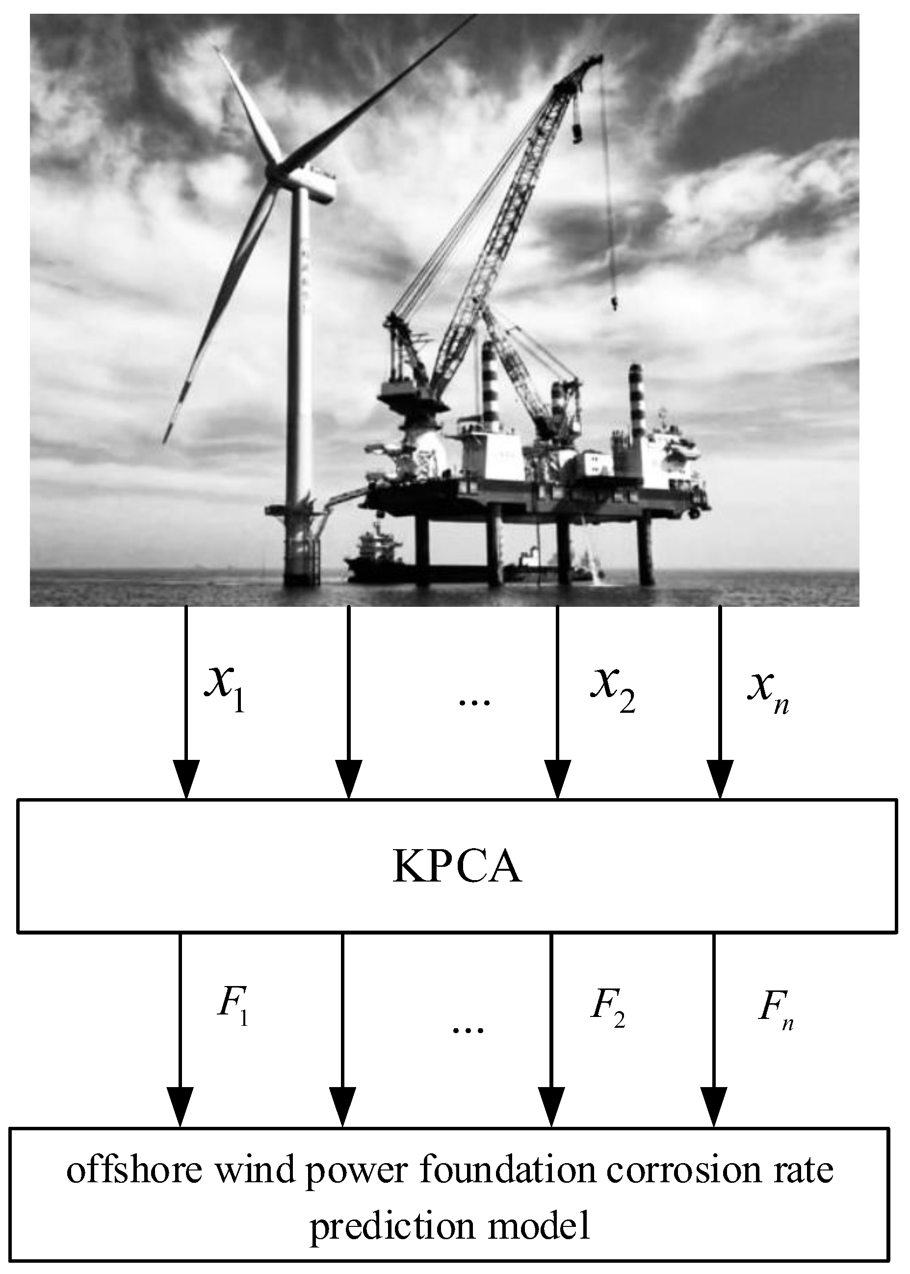
- The main elements of the offshore wind power foundation corrosion rate are extracted using kernel principal component analysis, which reduces the modeling workload of the offshore wind power foundation corrosion prediction model.
- (2)
- The improvement of the spotted hyena algorithm by the nonlinear adjustment of convergence factor and Lévy flight strategy, which accelerates the convergence speed of the algorithm and improves the optimization ability.
- (3)
- Based on the improved spotted hyena algorithm, the least squares support vector machine’s penalty parameter and kernel function parameter are optimized, and the offshore wind power foundation corrosion rate prediction model is established.
The organization of this paper is as follows: Section 1 analyzes the corrosion characteristics of offshore wind power foundations; Section 2 introduces the kernel principal component analysis method; Section 3 introduces the spotted hyena optimization algorithm improvement strategy; Section 4 introduces the corrosion rate prediction model for offshore wind power foundation based on ISHO-LSSVM; Section 5 is the simulation verification; and Section 6 is the conclusion.
2. Corrosion Characteristics of Offshore Wind Power Foundations
Single offshore wind turbine foundations and conduit frame foundations are mostly composed of steel structures, and the pile foundation of the high pile cap foundation is often made of steel pipe piles [21], as shown in Figure 1. The transition section and connection with the pile foundation are also often made of steel structures. It can be said that steel is the most important material used for offshore wind turbine foundations. The foundation stands tall in the marine environment and has strong corrosiveness to steel, similar to general marine structures. Its most prominent feature is the marine corrosion problem of steel. The corrosion resistance varies greatly with different exposure conditions. It is usually divided into five zones [22]. The presence of salt particles or salt mist in the marine atmospheric region leads to much greater corrosion in this area than inland areas. The splash zone has sufficient oxygen supply, sufficient sunlight, and a large amount of salt particles. During the process of dry–wet alternation and under the impact of waves, local corrosion is more severe, making it the area with the most severe corrosion.
Figure 1.
The offshore wind power foundation.
However, the wind turbine foundation, as the supporting structure of the wind turbine, is different from harbor structures or offshore platform structures, as it combines the characteristics of high-rise structures and power machine foundations [23]. The large overturning moment with the uncertain direction of the wind turbine foundation results in significant alternating tensile stress. At the same time, the structural components of the foundation not only bear the load of the marine environment but also the dynamic load generated during the operation of the wind turbine. The interweaving effect of stress and corrosion, as well as fatigue and corrosion, is more prominent. Once local damage occurs to the anti-corrosion protection system in important parts (such as the foundation node of the jacket), it is extremely easy to cause structural damage. Therefore, there is a higher demand for the reliability and corrosion rate prediction of anti-corrosion protection measures during the lifespan of wind turbine foundations.
3. Kernel Principal Component Analysis
In order to eliminate the effect of different magnitudes in the data set, the original data are normalized to obtain the new data set. The normalization formula is as follows [21]:
where is the normalized data; is the original data of an eigenvector; and are the maximum and minimum values of the eigenvector, respectively.
Mapping the new dataset to gain high-dimensional space , , the covariance matrix in the high-dimensional space is as follows [19]:
Let the kernel function be , where . Using the kernel function, the characteristic polynomial of the covariance can be simplified to obtain the following:
where α is a column vector of dimension n.
The cumulative contribution of each factor c is calculated, and the main influence factor can be determined by extracting the q main elements with higher contribution, and the formula for h is as follows [18]:
Usually, the requirement is satisfied when the cumulative contribution c is greater than 85% [14]. Using Equation (4) to determine the principal components, for any sample x, the reconstructed nonlinear sample Fi can be obtained by performing a high-dimensional mapping of its eigenvalue α and eigenvector ui as follows:
4. Spotted Hyena Optimization Algorithm Improvement Strategy
4.1. Spotted Hyena Optimization Algorithm
In 2018, the Indian scholar Gaurav Dhiman proposed the spotted hyena optimizer (SHO). The predatory process of the spotted hyena populations involves four stages. The principle of the SHO is as follows:
(1) Encirclement process: The spotted hyena is able to acutely perceive the location, which is as follows [14]:
where Dh is the distance; t is the number of iterations; Pp is the position of the prey; P(t) is the position; B is the swing factor; r1 is a uniformly distributed random number; r1 ∈ [0, 1].
The spotted hyena individual position update formula is as follows [6]:
where E is the convergence factor, r2 has the same meaning as r1, h is the control factor, and NI is the maximum number of iterations.
(2) Hunting process: The spotted hyenas belong to a group of animals and complete the hunt by trusting each other and exchanging information to determine the location of prey. This process is as follows [15]:
where Ph is the first optimal position; and Ch is the set containing N optimal solutions. Where the expression for N is as follows:
where M is a random vector in between [0.5, 1]; nos defines the number of feasible solutions.
(3) The process of attacking prey (local search): When hunting is completed, it starts to attack the prey, and the condition of attacking the prey is reached. The mathematical expression of this process is as follows:
where Ph(t + 1) is the preserved optimal solution.
(4) Search process (global search): The spotted hyena searches for the prey according to the position in the set of optimal solutions Ch. When the convergence factor is satisfied, it will spread out to search for the prey with a better position, which is a mechanism that facilitates the SHO to carry out global search.
Compared with other optimization algorithms, SHO has fewer parameters, simple operation, good stability, and higher solution accuracy. However, its optimization ability relies on the two random parameters B and E to regulate, and during the optimization process, the SHO also suffers from falling into local optimums and insufficient solution accuracy.
4.2. Nonlinear Adjustment of Convergence Factors
When the SHO is iteratively calculated, the control factor h adopts a linearly decreasing adjustment strategy, but in fact, the change in h is nonlinear; in order to better reflect the algorithm’s optimization process, this paper introduces a nonlinear adjustment strategy as follows [24,25,26]:
where e is the natural logarithm, Q is the attenuation coefficient, and the larger Q is, the more h attenuates.
Through the improvement, the control factor h realizes a nonlinear decrease from five to zero. At the beginning of the algorithm iteration, h is slowly decreasing, which is better decaying compared to the original control factor, and is favorable for the algorithm to perform the global search. In the late iteration, the improved h decays faster, which makes the population closer to the optimal solution.
4.3. Levi’s Flight Strategy
Lévy flight is a kind of non-Gaussian stochastic process, which is more stochastic and can explain certain stochastic phenomena in nature [22]. This kind of step size adjustment can not only increase the population diversity, but also help the population to reach the global optimal solution. Therefore, the introduction of the Lévy flight strategy in the optimization algorithm is conducive to increasing the population diversity and expanding the search range.
To enhance the optimization performance, the Lévy flight strategy is introduced in the SHO and acts on the stochastic factors r1 and r2 of the SHO as follows [15]:
The swing factor is defined as Equation (17):
The convergence factor is defined as Equation (18):
where Levy is the search path.
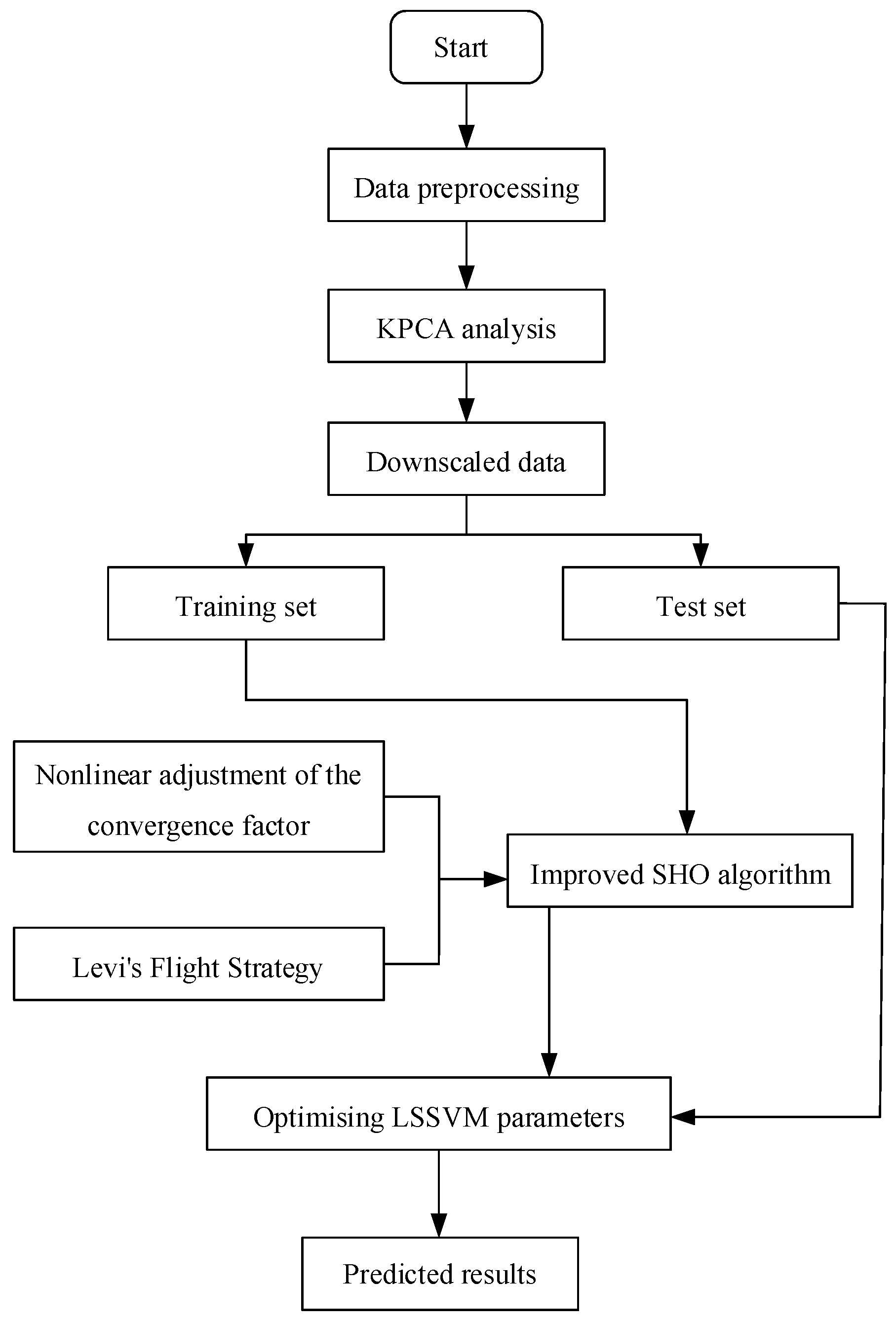
5. Corrosion Rate Prediction Model for Offshore Wind Power Foundation Based on ISHO-LSSVM
LSSVM is a machine learning method for solving nonlinear regression problems. LSSVM is characterized by the small number of samples required and high regression accuracy, and is now widely used to solve nonlinear regression problems [23].
For the acquired data sample set , where is the input quantity and is the output quantity. The objective function of LSSVM to solve the optimization problem is as follows:
where is the nonlinear mapping; is the hyperplane weight vector; b is the bias factor; C is the penalty coefficient; and is the slack variable.
Introducing the Lagrangian operator , the Lagrangian function is obtained as follows:
The partial derivatives of Equation (20) are solved, and then the substitutions in the partial derivatives are made to finally obtain the expression of the classification function of the LSSVM:
The penalty parameter C and the kernel function parameter are two very important parameters of LSSVM, which have a great influence on the regression fitting effect of LSSVM. In order to obtain a better fitting effect, it is necessary to find the optimization of C and . The ISHO-LSSVM prediction model is used to predict the current system state.
The corrosive environment of offshore wind power operation is very harsh; the high humidity and high salinity of the sea surface atmospheric area, the dry and wet alternation of the splash zone and tidal zone, and the seawater immersion and seabed attachment of the submerged area, and other harsh corrosive environments will cause serious corrosion hazards to the monopile foundation of the offshore wind turbine, and the environmental load of the monopile foundation is much higher than that of land, and its corrosion rate affects a large number of factors with a certain degree of correlation between the various factors. In order to reduce the modeling workload of the offshore wind turbine foundation corrosion prediction model, KPCA is used to process the corrosion rate influencing factors of the offshore wind turbine foundation, downsizing the sample data in high dimensional space, eliminating the spatial correlation and redundancy of data, and extracting the main data of the main nonlinear characteristics of the principal elements. Using the convergence factor nonlinear adjustment and Lévy flight strategy to improve SHO and improve the performance of SHO’s optimization, and using ISHO to optimize the parameters of LSSVM to establish the offshore wind power base corrosion rate prediction model based on the KPCA-ISHO-LSSVM, the modeling process is shown in Figure 2.
Figure 2.
Corrosion rate prediction model for offshore wind power foundation.
The steps for forecasting are as follows:
- (1)
- Obtain sample data. According to the factors affecting the corrosion rate of offshore wind power foundations, the relevant data are collected.
- (2)
- Normalization. To eliminate the error affected by the different scales of the influencing factors, the sample data are normalized to obtain the data set .
- (3)
- KPCA dimensionality reduction. KPCA is used to downsize the data set to obtain the reconstructed indexes .
- (4)
- ISHO parameter optimization. Use ISHO to optimize C and of LSSVM. The process of ISHO can be seen in Figure 3.
- (5)
- Set the initial values and search ranges of penalty parameters C and kernel function parameters, and set the population size of the spotted hyena.
- (6)
- Calculate the current optimal position and check if there are any spotted hyena individuals that are beyond the boundaries and adjust them if any.
- (7)
- Calculate the individual fitness value of the spotted hyena after the position update and compare it with the fitness value of the previous generation to retain the best position of the spotted hyena.
- (8)
- Update the group of spotted hyenas until the spotted hyena position under the individual optimal fitness value is searched.
- (9)
- If the algorithm reaches the termination condition, output the best spotted hyena position, i.e., the optimal solution of C and ; otherwise repeat steps (5) to (9).
- (10)
- The optimal solution of C and is assigned to LSSVM, which is utilized to predict the corrosion rate of offshore wind power foundations.
Figure 3.
Optimization flow chart of ISHO.
After the prediction is completed, the prediction model needs to be evaluated, and in this paper, the average relative error, the root mean square error, the global maximum relative error, and the coefficient of determination are used to make a comprehensive evaluation of the prediction effect of the model, and their calculation formulas are as follows:
where N is the sample capacity of the test set, is the actual value of corrosion rate, is the predicted value of corrosion rate, and is the average value of corrosion rate.
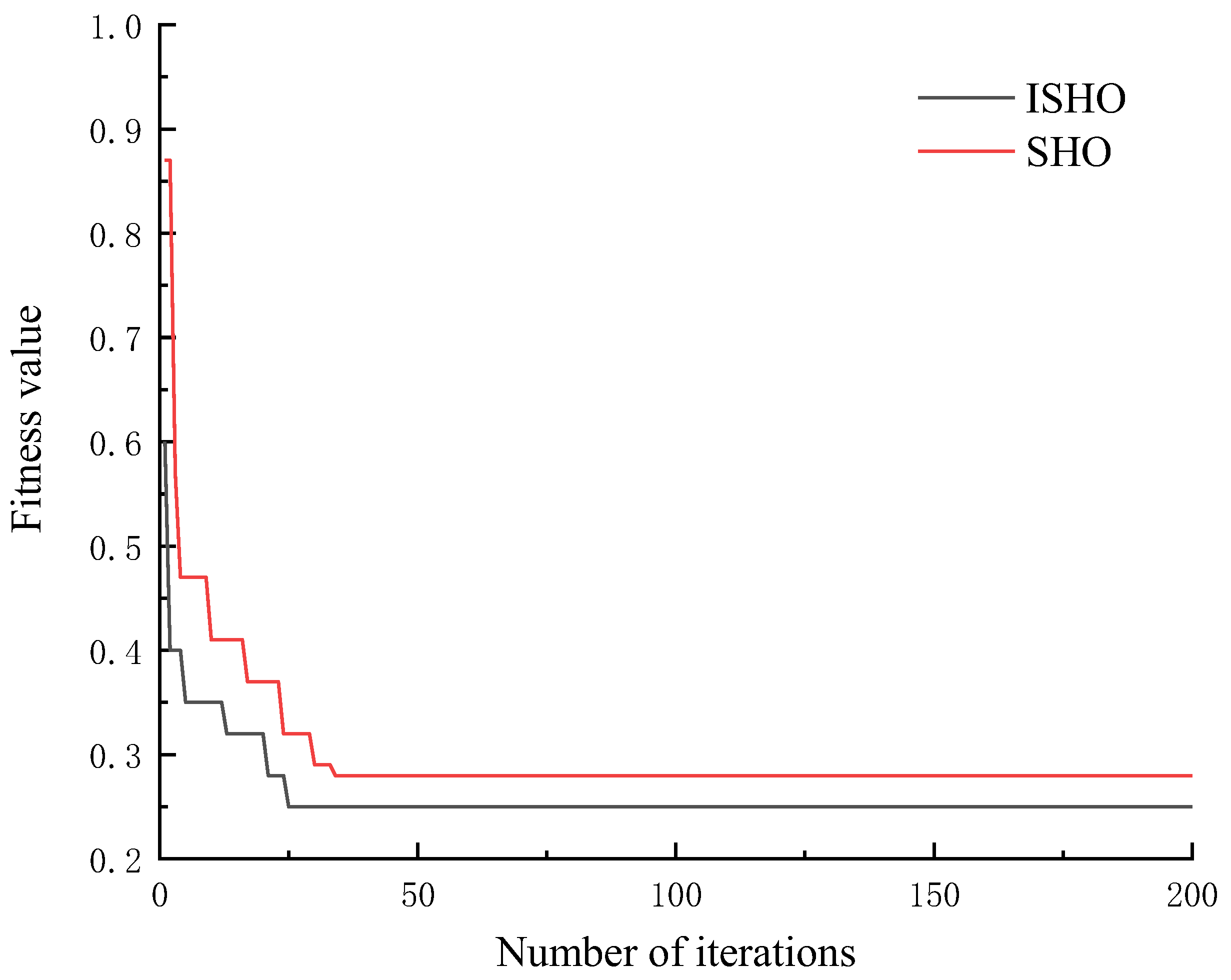
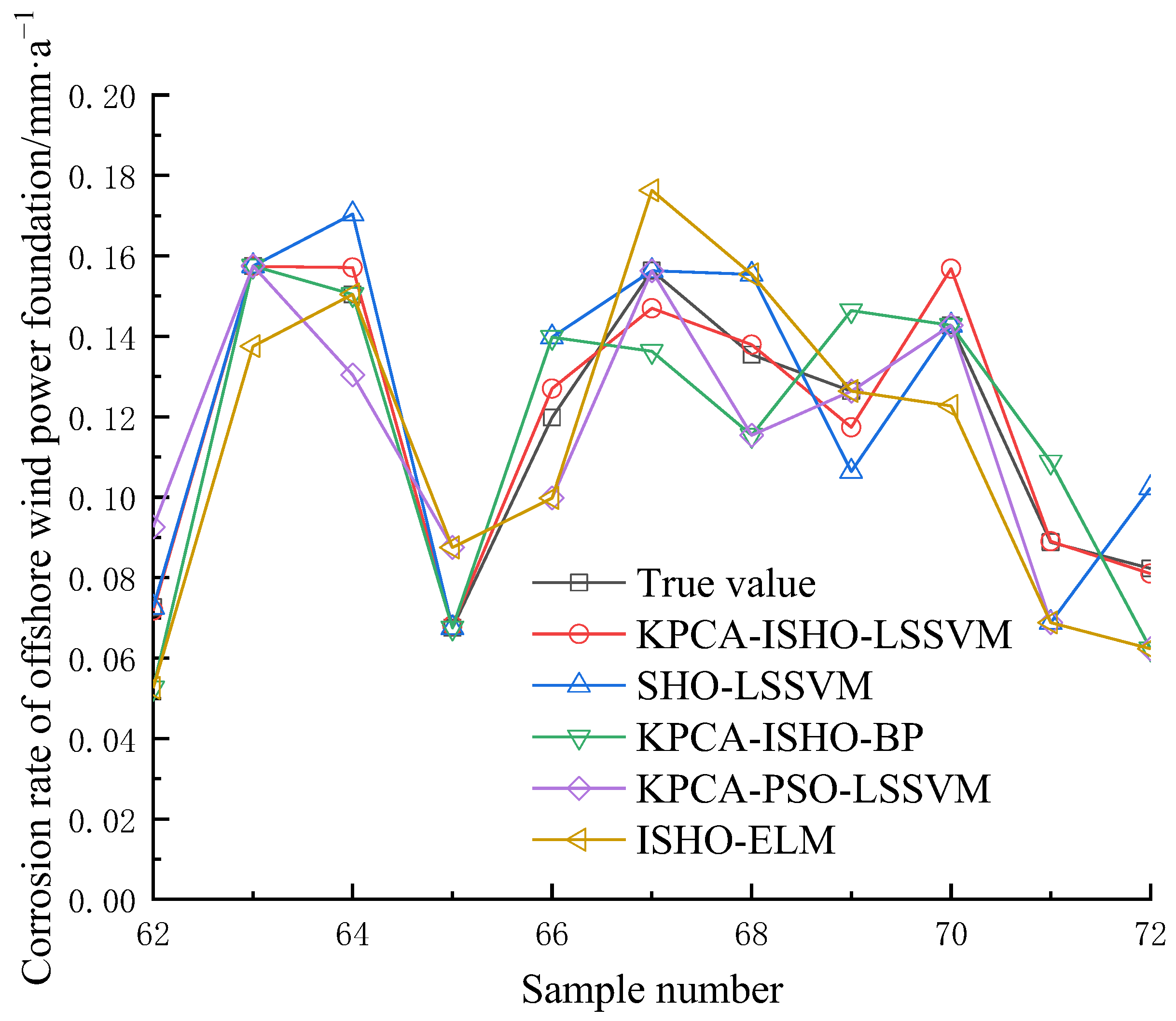
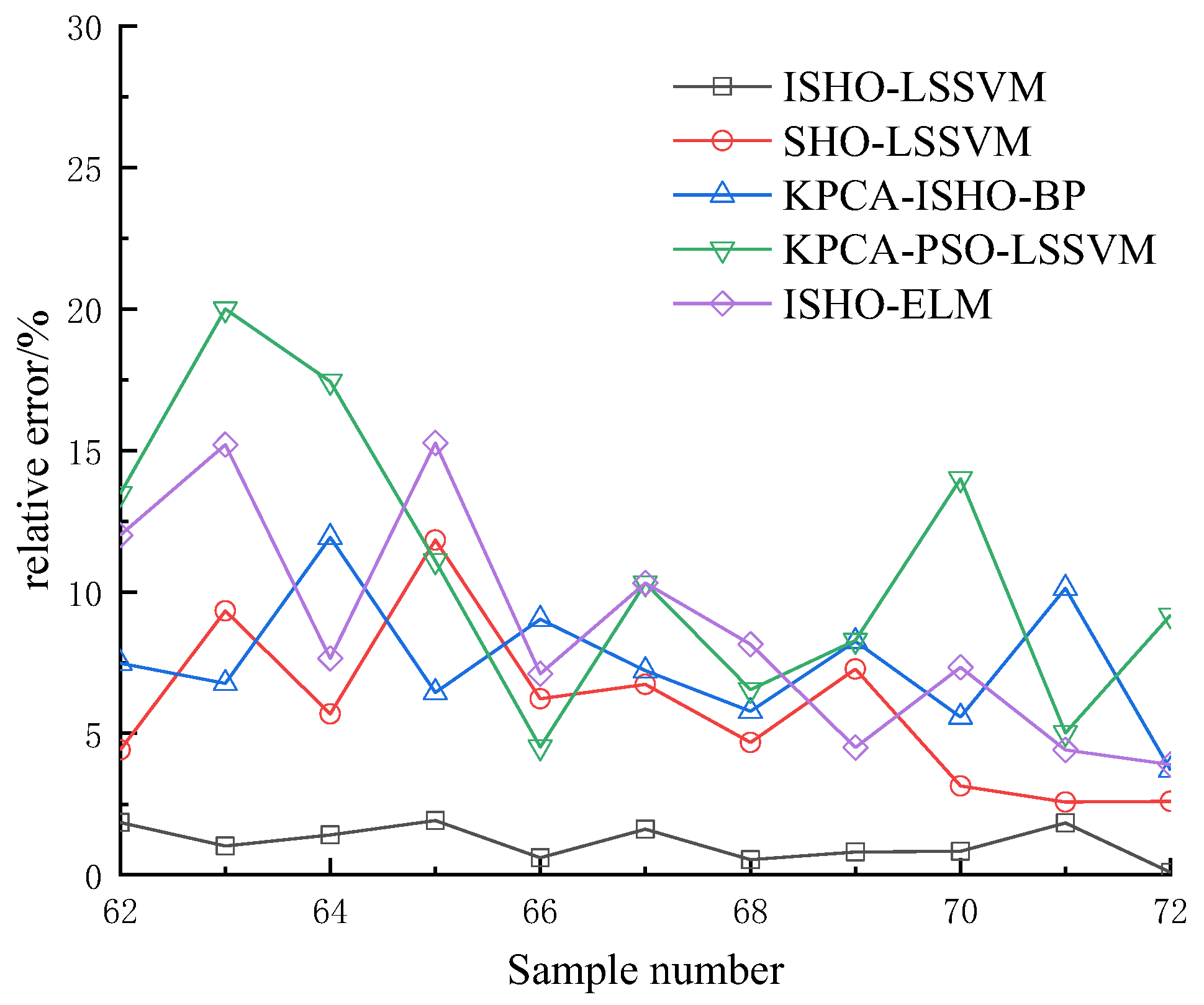
6. Experimental Verification and Analysis
To verify the effectiveness of the proposed approach, simulation analysis is carried out based on the actual collected data. Based on the data provided by the project “Aguiyang Engineering Corporation Limited Key Scientific Research Project (YJ2023-13)”, seawater data were collected from 15 offshore wind farms and 72 sets of sample data are shown in Table A1. The 72 sets of data were normalized based on Equation (1) due to the large magnitude differences between the different types of influencing factors. KPCA was used to calculate the cumulative contribution of each factor. The results of KPCA algorithm processing are shown in Table 1. The first 60 groups are regarded as the training set, while the last 10 groups are the test set, which can effectively evaluate and validate the generalization performance of models or algorithms based on this data while ensuring that the data are fully utilized.
Table 1.
Results of KPCA analyses.
According to the basic principle of the preferential selection of the kernel principal components of influencing factors using KPCA, if the sum of the contribution rates of some influencing factors exceeds 85%, these factors can be used instead of all the factors for the corrosion rate prediction study. As can be seen in Table 1, the cumulative contribution rate of PH value, , , , and has reached more than 85%. Therefore, these five influencing factors are selected as the key indicators of offshore wind power foundation corrosion for the next prediction study. According to the coefficient matrix of the principal components to reorganize the data, the sample data were reorganized from the previous eleven-dimensional data to five-dimensional data. The reorganized sample data are shown in Table A2.
Using the training set for training, the of the samples is used as the fitness function of the optimization objective, and the improved SHO algorithm is applied to optimize the C and of the LSSVM, with the initial values of the C and set to 100 and 1, respectively, and the search ranges are both [0, 1000]. The iteration curves of the ISHO and the SHO are shown in Figure 4.
Figure 4.
Iterative curve of ISHO and SHO.
In Figure 4, the fitness value of each algorithm decreases with the increase in iteration number, but ISHO can achieve the minimum mean square error in fewer iterations. SHO also achieves a better fitness value in fewer iterations, but the ability to find the optimal solution is still inferior to that of ISHO. The initial fitness value of ISHO is lower than that of SOA, which indicates that after the optimization of Lévy’s flight strategy, the initial positional quality of the population has been improved. ISHO reaches the minimum fitness value after 25 iterations, when the corresponding optimal solutions C and are 58.47 and 2.16, respectively.
The optimal values C = 58.47 and = 2.16 found by ISHO are assigned to LSSVM to predict the test set data. To further validate the superiority of the offshore wind power base corrosion rate prediction method based on the KPCA-ISHO-LSSVM model, comparative analyses are conducted with the KPCA-SHO-LSSVM, KPCA-ISHO-BP, KPCA-PSO-LSSVM, and ISHO-ELM models. The settings of SHO and LSSVM in the SHO-LSSVM model are consistent with this study; the settings of KPCA and ISHO in the KPCA-ISHO-BP model are consistent with this study, and the BP network structure is 3-9-1; the settings of KPCA and LSSVM in the KPCA-PSO-LSSVM model are consistent with this study, and the PSO parameters of the search space dimension are 2, the weight factor is 2, and the acceleration factor is 0.9 and 0.4, respectively; and the ISHO-ELM model settings are consistent with this study, and the ELM model network structure is 10-28-1. The prediction results are shown in Figure 5 and Table 2.
Figure 5.
Corrosion rate prediction results of offshore wind power foundation with different prediction methods.
Table 2.
Results of model evaluation indicators.
In Figure 5, the SHO-LSSVM model shows the highest prediction error, primarily due to its longer computation time and vulnerability to dimensional explosion and catastrophe. In addition, the prediction accuracy of the ISHO-ELM model is slightly worse compared to KPCA-PSO-LSSVM and KPCA-ISO-BP. This is related to the poor mapping effect of the ELM model in dealing with high-dimensional data, which does not retain the hidden variable information well and cannot express the nonlinear dependencies well, resulting in biased prediction results. Compared with KPCA-SHO-LSSVM, KPCA-ISO-BP, KPCA-PSO-LSSVM, and ISHO-ELM, the predicted values of the improved pre-prediction method in this paper match the actual values better. This indicates that by using the kernel function to map the sample data into the high-dimensional space and finding its subspace in the high-dimensional space for dimensionality reduction, the main element extraction accuracy is higher, effectively reducing the redundancy of the data features and improving the prediction effect of the model. Comparing the prediction effect before and after the improvement of the algorithm, it can be seen that the improved algorithm has higher prediction accuracy, improves the speed and accuracy of the model solution, and does not fall into the situation of local optimization.
To make a reasonable evaluation of the prediction accuracy of the combination model proposed in this study, this combination model is comprehensively compared with other common models, and the error changes are shown in Figure 6.
Figure 6.
Comparison of prediction errors of various models.
Through comparison, it can be found in Figure 6 that the errors of each group of the prediction results of the combined model proposed in this study are smaller than the other five models. The maximum relative error is less than 4%, which proves that its generalization ability is relatively good. The results of the various types of prediction errors and the coefficients of determination of the models of the five prediction models are shown in Table 2.
In Table 2, for the training set data, the ISHO-LSSVM model has a smaller error, a larger coefficient of determination, and a better training effect than the other models. For the test set data, the , , and index of the ISHO-LSSVM model are smaller than the other three prediction models, in which the average relative error is 2.86%, which is 54.7% less than that of the SHO-LSSVM model, which shows that the model prediction accuracy is higher; the and are 0.15 and 3.74%, respectively, which are 80.5% and 62.5% less than the SHO-LSSVM model. It can be seen that the volatility of the model prediction is smaller; from the coefficient of determination, the coefficient of determination of the ISHO-LSSVM model is 0.995, which is larger than that of the other three models. In summary, the corrosion rate prediction method of offshore wind power based on KPCA-ISHO-LSSVM proposed in this paper can further improve the corrosion rate prediction accuracy, and verify the correctness and superiority of the proposed corrosion rate prediction model.
7. Conclusions
In this paper, an offshore wind power foundation corrosion rate prediction method is proposed. The principal elements of offshore wind power foundation corrosion rate are extracted using the kernel principal component analysis, and the new dataset is mapped to a high-dimensional space by mapping function, which reduces the modeling workload of the offshore wind power foundation corrosion prediction model. The SHO algorithm is improved by the convergence factor nonlinear adjustment and Lévy flight strategy, and the penalty parameters and kernel function parameters of the least squares support vector machine are optimized based on the improved spotted hyena algorithm. The simulation results are as follows:
(1) With the KPCA approach, it is found that for the offshore wind power foundation, , , , and are some of the factors that have the greatest impact on corrosion. The data dimensionality reduction, under the premise of guaranteeing the prediction accuracy, effectively simplifies the network structure of the corrosion rate prediction model, greatly reducing its arithmetic volume and speeding up the calculation speed.
(2) The SHO algorithm is improved by the convergence factor nonlinear adjustment and Lévy flight strategy, and it is used to optimize the LSSVM model, which improves the convergence speed and prediction accuracy. The algorithm reaches the minimum fitness value after 25 iterations. The average relative error, root mean square error, and global maximum relative error homogenization coefficients of the combined prediction model in this paper are 2.86%, 0.15, 3.74%, and 0.995, respectively, which are better than those of the other corrosion prediction models.
With the approach proposed in this paper, we can grasp the foundation’s health state for offshore wind turbines’ operational safety. Due to the complexity and variability of the marine environment, more factors affect the corrosion rate of the substrate, and certain indicators are difficult to measure and quantify. In future research, the matrix corrosion data will be analyzed and predicted based on comprehensive indicators to improve the accuracy of the corrosion rate prediction further. At the same time, after obtaining accurate corrosion rate prediction results, it is necessary to carry out subsequent corrosion prevention design. The development of anti-corrosion measures will be studied in the future.
Author Contributions
Conceptualization, F.Z. (Fan Zhang) and F.Z. (Feng Zhang); methodology, F.Z. (Feng Zhang) and H.M.; software, H.W. and H.Z.; validation, H.Z.; formal analysis, F.Z. (Feng Zhang); investigation, H.Z.; writing—original draft preparation, F.Z. (Fan Zhang), F.Z. (Feng Zhang), H.M., H.W. and H.Z. All authors have read and agreed to the published version of the manuscript.
Funding
This research is funded by the Guiyang Engineering Corporation Limited Key Scientific Research Project (Yj2023-13).
Data Availability Statement
The original contributions presented in the study are included in the article, further inquiries can be directed to the corresponding authors.
Conflicts of Interest
Author Feng Zhang was employed by the Power China GuiYang Engineering Corporation Limited. The remaining authors declare that the research was conducted in the absence of any commercial or financial relationships that could be construed as a potential conflict of interest.
Nomenclature
| the normalized data | |
| the original data of an eigenvector | |
| , | the maximum and minimum values of the eigenvector, respectively |
| α | the column vector of dimension n |
| Dh | the distance |
| t | the number of iterations |
| Pp | the position of the prey |
| P(t) | the position |
| B | the swing factor |
| r1 | a uniformly distributed random number |
| E | the convergence factor |
| h | the control factor |
| NI | the maximum number of iterations |
| Ph | the first optimal position |
| Ch | the set containing N optimal solutions |
| M | the random vector |
| Ph(t + 1) | the preserved optimal solution |
| e | the natural logarithm |
| Q | the attenuation coefficient |
| the nonlinear mapping | |
| the hyperplane weight vector | |
| b | the bias factor |
| C | the penalty coefficient |
| the slack variable | |
| N | the sample capacity of the test set |
| the actual value of corrosion rate | |
| the predicted value of corrosion rate | |
| the average value of corrosion rate |
Appendix A
Table A1.
Seventy-two sets of raw sample data.
Table A1.
Seventy-two sets of raw sample data.
| Sample No. | PH Value | ||||||||||
|---|---|---|---|---|---|---|---|---|---|---|---|
| 1 | 7.91 | 2238.26 | 348.16 | 206.55 | 129.82 | 1.31 | 44.45 | 1327.28 | 323.16 | 116.83 | 0.24 |
| 2 | 7.66 | 2036.13 | 379.93 | 200.26 | 203.27 | 7.13 | 31.90 | 1260.06 | 301.21 | 135.37 | 0.73 |
| 3 | 7.66 | 2126.99 | 324.64 | 230.65 | 204.24 | 3.75 | 38.32 | 1235.92 | 282.76 | 139.21 | 0.66 |
| 4 | 7.11 | 2079.74 | 280.90 | 184.18 | 112.17 | 5.86 | 32.61 | 1095.35 | 275.83 | 109.75 | 0.14 |
| 5 | 8.20 | 2203.06 | 356.86 | 180.34 | 75.95 | 3.32 | 34.89 | 1200.45 | 272.87 | 126.43 | 0.07 |
| 6 | 8.05 | 2092.34 | 352.99 | 194.56 | 71.73 | 2.72 | 33.33 | 1110.04 | 277.56 | 148.75 | 0.11 |
| 7 | 8.42 | 2093.29 | 378.85 | 199.96 | 149.55 | 3.72 | 37.33 | 1110.89 | 270.35 | 135.10 | 0.40 |
| 8 | 7.58 | 2251.04 | 307.69 | 200.04 | 139.15 | 4.67 | 44.29 | 1182.38 | 268.61 | 166.55 | 0.11 |
| 9 | 8.25 | 2009.35 | 350.50 | 215.10 | 213.20 | 8.32 | 33.81 | 1185.95 | 251.53 | 164.80 | 0.39 |
| 10 | 7.23 | 2269.88 | 289.54 | 187.51 | 160.54 | 6.79 | 41.89 | 1005.79 | 275.46 | 132.85 | 0.23 |
| 11 | 8.36 | 2150.76 | 389.83 | 227.22 | 196.36 | 7.99 | 42.12 | 1337.89 | 278.20 | 115.25 | 0.31 |
| 12 | 8.45 | 2165.70 | 388.05 | 226.22 | 152.89 | 5.51 | 41.42 | 1121.73 | 332.87 | 177.63 | 0.14 |
| 13 | 7.06 | 2041.95 | 338.46 | 235.14 | 88.61 | 8.40 | 35.78 | 1206.93 | 313.07 | 128.07 | 0.50 |
| 14 | 8.39 | 2034.41 | 315.73 | 223.75 | 70.53 | 2.45 | 35.02 | 1143.15 | 272.08 | 112.30 | 0.46 |
| 15 | 7.11 | 2014.69 | 344.74 | 219.18 | 205.04 | 9.49 | 41.48 | 1161.25 | 295.00 | 173.66 | 0.01 |
| 16 | 8.17 | 2158.54 | 347.08 | 214.58 | 128.94 | 3.54 | 34.61 | 1099.25 | 309.11 | 148.48 | 0.15 |
| 17 | 8.11 | 2045.60 | 305.14 | 224.61 | 80.67 | 9.38 | 33.86 | 1348.56 | 290.87 | 112.99 | 0.10 |
| 18 | 7.38 | 2072.77 | 375.27 | 212.90 | 165.36 | 8.94 | 42.57 | 1000.23 | 293.01 | 139.10 | 0.41 |
| 19 | 8.26 | 2346.29 | 299.24 | 180.61 | 137.91 | 5.15 | 31.60 | 1051.99 | 271.93 | 137.06 | 0.56 |
| 20 | 8.32 | 2342.69 | 379.39 | 197.19 | 197.74 | 5.77 | 44.45 | 1026.08 | 329.00 | 168.69 | 0.12 |
| 21 | 7.58 | 2229.56 | 347.49 | 238.50 | 93.39 | 7.74 | 36.24 | 1211.59 | 319.43 | 144.41 | 0.19 |
| 22 | 7.11 | 2117.48 | 300.45 | 181.01 | 164.68 | 5.66 | 34.89 | 1142.87 | 271.17 | 128.07 | 0.41 |
| 23 | 7.29 | 2174.76 | 365.91 | 192.76 | 101.16 | 2.72 | 41.88 | 1182.86 | 251.45 | 112.10 | 0.56 |
| 24 | 7.13 | 2304.59 | 340.51 | 222.32 | 178.80 | 3.57 | 42.64 | 1137.51 | 257.50 | 174.07 | 0.35 |
| 25 | 7.79 | 2066.46 | 300.06 | 175.50 | 105.44 | 6.86 | 43.55 | 1178.54 | 291.39 | 119.55 | 0.11 |
| 26 | 8.29 | 2090.58 | 352.56 | 209.19 | 145.48 | 5.40 | 35.14 | 1127.39 | 275.18 | 135.26 | 0.56 |
| 27 | 8.15 | 2025.40 | 318.88 | 195.57 | 152.68 | 7.32 | 39.50 | 1013.45 | 303.50 | 167.91 | 0.58 |
| 28 | 7.86 | 2252.02 | 366.31 | 234.50 | 161.86 | 4.54 | 41.84 | 1025.18 | 301.61 | 160.49 | 0.57 |
| 29 | 8.25 | 2221.12 | 352.78 | 181.18 | 86.58 | 9.05 | 43.93 | 1310.35 | 271.39 | 179.89 | 0.24 |
| 30 | 7.07 | 2121.29 | 304.09 | 177.98 | 171.63 | 9.42 | 30.59 | 1239.06 | 329.98 | 164.17 | 0.17 |
| 31 | 7.28 | 2057.52 | 384.06 | 238.16 | 105.97 | 6.11 | 37.01 | 1259.99 | 275.26 | 143.48 | 0.40 |
| 32 | 7.15 | 2078.03 | 354.04 | 201.38 | 197.13 | 5.86 | 30.92 | 1304.22 | 300.91 | 183.60 | 0.39 |
| 33 | 7.95 | 2096.11 | 351.18 | 210.37 | 127.33 | 3.08 | 35.87 | 1302.04 | 323.26 | 103.43 | 0.19 |
| 34 | 8.29 | 2076.18 | 377.74 | 185.71 | 183.33 | 6.28 | 44.90 | 1066.20 | 267.38 | 174.57 | 0.47 |
| 35 | 7.20 | 2258.74 | 356.25 | 198.95 | 179.97 | 2.54 | 34.81 | 1264.56 | 293.88 | 181.48 | 0.32 |
| 36 | 7.46 | 2110.75 | 332.17 | 228.98 | 173.39 | 5.22 | 34.56 | 1316.49 | 321.35 | 168.06 | 0.21 |
| 37 | 7.98 | 2043.77 | 339.98 | 171.12 | 127.01 | 4.81 | 43.45 | 1330.64 | 297.69 | 123.32 | 0.55 |
| 38 | 7.99 | 2346.96 | 294.51 | 220.46 | 174.67 | 2.11 | 34.16 | 1190.28 | 268.59 | 108.87 | 0.28 |
| 39 | 7.89 | 2340.17 | 321.24 | 231.59 | 110.50 | 8.58 | 32.79 | 1336.60 | 294.30 | 126.18 | 0.10 |
| 40 | 8.24 | 2173.86 | 285.35 | 232.50 | 162.94 | 3.69 | 44.44 | 1290.95 | 274.93 | 160.94 | 0.19 |
| 41 | 7.42 | 2130.65 | 368.97 | 215.50 | 156.55 | 4.38 | 32.93 | 1197.14 | 260.17 | 181.86 | 0.12 |
| 42 | 7.11 | 2263.43 | 367.82 | 197.49 | 135.18 | 8.17 | 30.92 | 1018.90 | 266.40 | 134.82 | 0.17 |
| 43 | 7.17 | 2070.97 | 386.19 | 233.17 | 77.63 | 3.45 | 30.76 | 1216.82 | 273.08 | 155.66 | 0.46 |
| 44 | 7.80 | 2276.86 | 320.24 | 229.05 | 179.89 | 9.24 | 41.16 | 1023.68 | 322.32 | 173.73 | 0.41 |
| 45 | 7.21 | 2046.12 | 288.48 | 171.78 | 149.41 | 9.95 | 38.02 | 1129.15 | 301.83 | 118.52 | 0.25 |
| 46 | 8.19 | 2251.92 | 364.10 | 228.78 | 212.03 | 7.75 | 33.58 | 1096.08 | 267.93 | 161.85 | 0.13 |
| 47 | 7.20 | 2265.67 | 351.33 | 208.22 | 146.93 | 9.97 | 34.25 | 1251.08 | 255.02 | 147.07 | 0.21 |
| 48 | 8.09 | 2263.75 | 388.69 | 172.11 | 144.19 | 6.15 | 40.47 | 1272.56 | 304.71 | 112.48 | 0.24 |
| 49 | 7.67 | 2297.51 | 321.39 | 229.37 | 75.48 | 3.97 | 41.28 | 1264.80 | 267.92 | 104.53 | 0.10 |
| 50 | 7.81 | 2043.87 | 314.92 | 191.69 | 70.78 | 5.84 | 31.59 | 1174.21 | 303.64 | 138.71 | 0.57 |
| 51 | 8.19 | 2129.47 | 287.58 | 234.90 | 173.18 | 9.87 | 39.36 | 1172.94 | 315.14 | 128.88 | 0.20 |
| 52 | 7.53 | 2104.12 | 346.24 | 198.08 | 207.96 | 9.84 | 36.55 | 1234.40 | 258.62 | 126.66 | 0.55 |
| 53 | 7.67 | 2036.26 | 388.39 | 200.50 | 144.44 | 3.95 | 32.09 | 1340.48 | 269.20 | 101.94 | 0.46 |
| 54 | 8.48 | 2030.80 | 386.03 | 208.92 | 107.70 | 6.28 | 34.10 | 1113.40 | 285.19 | 176.82 | 0.27 |
| 55 | 8.14 | 2161.99 | 372.01 | 228.92 | 71.83 | 5.12 | 38.02 | 1147.17 | 309.01 | 104.46 | 0.52 |
| 56 | 7.53 | 2238.30 | 356.86 | 230.48 | 106.66 | 9.99 | 43.21 | 1016.68 | 258.10 | 118.04 | 0.16 |
| 57 | 7.32 | 2293.92 | 376.84 | 205.78 | 142.10 | 8.67 | 36.28 | 1067.72 | 284.13 | 129.92 | 0.17 |
| 58 | 7.74 | 2032.72 | 330.86 | 228.04 | 176.36 | 7.27 | 42.01 | 1257.12 | 250.49 | 155.79 | 0.19 |
| 59 | 7.14 | 2251.72 | 328.00 | 189.51 | 88.31 | 9.81 | 35.57 | 1169.14 | 278.13 | 116.77 | 0.24 |
| 60 | 7.08 | 2091.21 | 349.00 | 215.91 | 201.05 | 3.67 | 41.83 | 1316.71 | 291.07 | 167.70 | 0.28 |
| 61 | 8.29 | 2117.25 | 358.03 | 212.61 | 120.57 | 6.68 | 44.92 | 1002.34 | 321.71 | 140.49 | 0.12 |
| 62 | 8.41 | 2127.78 | 284.88 | 181.71 | 159.75 | 8.55 | 41.45 | 1110.21 | 258.29 | 184.98 | 0.18 |
| 63 | 7.74 | 2313.92 | 345.67 | 225.29 | 122.94 | 2.31 | 34.14 | 1079.63 | 256.49 | 102.50 | 0.28 |
| 64 | 7.93 | 2031.73 | 343.09 | 197.34 | 109.36 | 8.47 | 40.11 | 1175.68 | 304.94 | 163.11 | 0.15 |
| 65 | 7.84 | 2333.33 | 301.16 | 200.82 | 206.99 | 4.05 | 39.85 | 1098.16 | 255.61 | 155.94 | 0.49 |
| 66 | 7.45 | 2011.62 | 382.75 | 178.74 | 99.49 | 3.77 | 33.53 | 1192.98 | 304.10 | 125.90 | 0.60 |
| 67 | 8.35 | 2113.42 | 336.93 | 236.25 | 165.39 | 9.06 | 44.75 | 1121.94 | 309.74 | 114.10 | 0.24 |
| 68 | 7.98 | 2314.67 | 331.24 | 218.33 | 97.02 | 6.41 | 40.35 | 1125.20 | 299.20 | 138.92 | 0.21 |
| 69 | 7.58 | 2226.41 | 305.70 | 208.50 | 77.43 | 2.31 | 33.74 | 1228.85 | 301.13 | 148.67 | 0.11 |
| 70 | 7.77 | 2326.32 | 327.45 | 185.25 | 198.94 | 4.25 | 30.83 | 1139.43 | 305.80 | 126.63 | 0.26 |
| 71 | 8.32 | 2297.34 | 303.43 | 177.62 | 186.81 | 7.62 | 32.86 | 1256.10 | 322.48 | 117.24 | 0.25 |
| 72 | 8.46 | 2010.86 | 352.25 | 193.70 | 142.60 | 2.80 | 41.04 | 1335.83 | 315.15 | 104.43 | 0.29 |
Table A2.
Sample data after reorganization.
Table A2.
Sample data after reorganization.
| Sample No. | PH Value | ||||
|---|---|---|---|---|---|
| 1 | 3.8667 | 1.4723 | 1.5334 | 1.7113 | 1.1347 |
| 2 | 0.9639 | 3.3851 | −0.5092 | 1.3585 | 1.9899 |
| 3 | 3.2178 | 1.2275 | 4.5877 | 1.8631 | 1.8452 |
| 4 | 3.6379 | 1.3956 | 3.2653 | 2.6756 | 0.0835 |
| 5 | 2.6605 | 1.4138 | 0.8012 | −0.3450 | −1.6430 |
| 6 | −0.7152 | 0.6434 | 1.2457 | 4.5684 | −0.2847 |
| 7 | 2.7125 | 1.4111 | 1.3295 | −0.0465 | 3.1502 |
| 8 | 1.4475 | 1.4377 | 1.0151 | −0.3530 | 1.6834 |
| 9 | 1.3440 | 2.3981 | 1.2038 | 0.6798 | 3.9931 |
| 10 | 1.5487 | 1.4955 | 3.8252 | 3.5191 | 1.3049 |
| 11 | 1.1278 | 4.4259 | 4.0803 | −0.0458 | 2.4452 |
| 12 | 1.8761 | 1.9738 | 1.8543 | 0.8789 | −0.1415 |
| 13 | 1.0710 | 1.3474 | −0.8690 | 1.4715 | −0.6221 |
| 14 | −0.5449 | 1.8240 | 0.2439 | 0.7325 | 3.3775 |
| 15 | 2.5506 | 1.3922 | 1.2119 | 4.1506 | 1.1611 |
| 16 | 1.9410 | 1.0044 | 1.0387 | 1.9385 | 3.7135 |
| 17 | −1.1983 | 4.2355 | 3.8587 | 1.5143 | 3.8503 |
| 18 | 1.4657 | 2.8330 | 4.5500 | −1.4133 | 2.1842 |
| 19 | 1.6368 | 0.4111 | 1.2701 | 3.8163 | 3.2054 |
| 20 | −0.0681 | 2.0270 | 0.5875 | 0.1574 | 1.4655 |
| 21 | 1.3528 | 3.6093 | 1.6547 | 1.6997 | 3.5525 |
| 22 | 1.0196 | −0.9618 | 1.1812 | 2.3189 | 1.0002 |
| 23 | −0.6334 | 3.4965 | 1.7354 | −1.2712 | −0.1615 |
| 24 | 0.8840 | 2.5330 | 1.4664 | 0.1676 | 0.4845 |
| 25 | 1.2855 | −0.7190 | 3.6406 | 1.8047 | 1.4044 |
| 26 | 1.5093 | 1.9563 | 2.5178 | 1.0232 | 2.3792 |
| 27 | 0.1170 | 4.1509 | 3.6051 | 1.8205 | 0.1858 |
| 28 | 4.3603 | 3.4290 | 1.9341 | 1.1619 | 1.8012 |
| 29 | 1.3271 | 2.0159 | 1.7142 | 3.0885 | 1.3008 |
| 30 | 4.1483 | 1.9901 | −1.7808 | 1.4474 | 1.9034 |
| 31 | 1.2267 | 1.3241 | 4.0494 | 0.5719 | 1.5424 |
| 32 | 1.5910 | 4.1414 | 1.4887 | 1.9710 | 2.0941 |
| 33 | 1.0090 | 1.3422 | 2.2230 | 2.5956 | 4.3108 |
| 34 | −0.5153 | 1.4028 | 0.8700 | 2.4284 | 0.4382 |
| 35 | −0.5839 | 1.3993 | 0.3940 | −0.5932 | 1.2052 |
| 36 | 3.3077 | 2.4555 | 0.5273 | 1.6901 | 4.3718 |
| 37 | 1.8809 | 0.3851 | 1.3116 | 1.4645 | 3.8325 |
| 38 | −1.2419 | −0.8737 | 0.4045 | 0.4332 | −1.3403 |
| 39 | 4.5197 | 2.4452 | −0.5362 | 1.8641 | −1.3256 |
| 40 | 2.9916 | −0.3838 | −1.4375 | 3.9473 | −1.2102 |
| 41 | 1.8133 | 1.6818 | 1.4645 | −1.0576 | 1.5785 |
| 42 | 1.5323 | 1.9895 | −0.4454 | 2.5103 | 2.9246 |
| 43 | 0.3773 | 3.2531 | 0.1623 | −1.2305 | 1.5117 |
| 44 | 1.7237 | 1.5461 | 1.2343 | 2.9519 | 1.2744 |
| 45 | 2.7996 | 1.1701 | 1.3667 | 1.7061 | 1.5965 |
| 46 | 3.3535 | 0.6347 | 2.3013 | 1.3888 | 1.9898 |
| 47 | 3.5015 | 1.8914 | 1.7656 | 3.3636 | 1.9091 |
| 48 | −0.4978 | 1.8224 | −1.1664 | 4.2226 | 1.4734 |
| 49 | 1.8082 | −0.0855 | −0.6743 | −0.1832 | −0.7854 |
| 50 | 2.8001 | 0.7136 | 2.7971 | 1.4468 | 0.2061 |
| 51 | −0.1693 | 1.0677 | 1.5799 | 0.9540 | 4.1168 |
| 52 | 1.3731 | 3.9771 | −1.0960 | 3.4502 | −0.9775 |
| 53 | −0.9404 | 4.7953 | 3.3717 | 1.3110 | 4.7877 |
| 54 | 3.4656 | 1.5696 | 3.8690 | 1.3556 | 1.9154 |
| 55 | 1.3066 | 0.3734 | 4.6552 | −0.9089 | 3.8551 |
| 56 | 1.3848 | 1.0737 | −0.7851 | 0.0726 | −1.2623 |
| 57 | −0.5064 | 1.3327 | 1.1752 | 1.0100 | 1.0897 |
| 58 | −0.8443 | −0.0952 | −0.0844 | 1.4798 | 1.7999 |
| 59 | −0.6794 | −0.3741 | 0.2110 | 3.2230 | 4.0719 |
| 60 | 3.7750 | 2.2032 | 0.6601 | 1.9699 | 3.4242 |
| 61 | 1.9985 | 1.5485 | 3.8154 | 1.8493 | 4.4840 |
| 62 | −0.5110 | 1.2685 | 1.9218 | −1.0822 | 2.1844 |
| 63 | 1.1061 | 1.2407 | 2.2131 | 0.9143 | 1.3326 |
| 64 | 3.4188 | 1.3210 | 1.1136 | 2.6456 | −0.6040 |
| 65 | −1.5663 | 1.3232 | 2.1802 | 1.3925 | 0.3722 |
| 66 | 1.5363 | −0.3021 | −0.2141 | −0.4896 | 1.6825 |
| 67 | 2.7397 | 1.9967 | 1.3049 | −0.1274 | 0.7298 |
| 68 | 1.4288 | 2.7448 | 1.7961 | 1.9226 | 1.0469 |
| 69 | 1.2406 | 3.8171 | 0.1451 | 1.8871 | −0.2190 |
| 70 | 1.4798 | 1.1895 | 3.9302 | 1.0689 | 1.3047 |
| 71 | 1.1092 | 1.7501 | 1.8874 | 4.0020 | −0.2864 |
| 72 | −1.0091 | 1.0085 | 1.0856 | 0.6599 | 2.6047 |
References
- Ariae, A.R.; Jahangiri, M.; Fakhr, M.H.; Shamsabadi, A.A. Simulation of biogas utilization effect on the economic efficiency and greenhouse gas emission: A case study in Isfahan, Iran. Int. J. Renew. Energy Dev. 2019, 8, 149–160. [Google Scholar] [CrossRef]
- Siampour, L.; Vahdatpour, S.; Jahangiri, M.; Mostafaeipour, A.; Goli, A.; Shamsabadi, A.A.; Atabani, A. Techno-enviro assessment and ranking of Turkey for use of home-scale solar water heaters. Sustain. Energy Technol. Assess. 2020, 43, 100948. [Google Scholar] [CrossRef]
- Yang, L.; Li, H.; Zhang, H.; Wu, Q.; Cao, X. Stochastic-Distributionally Robust Frequency-Constrained Optimal Planning for an Isolated Microgrid. IEEE Trans. Sustain. Energy 2024. [Google Scholar] [CrossRef]
- Alayi, R.; Jahangiri, M.; Guerrero, J.W.G.; Akhmadeev, R.; Shichiyakh, R.A.; Zanghaneh, S.A. Modelling and reviewing the reliability and multi-objective optimization of wind-turbine system and photovoltaic panel with intelligent algorithms. Clean Energy 2021, 5, 713–730. [Google Scholar] [CrossRef]
- Chui, K.T.; Gupta, B.B.; Vasant, P. A genetic algorithm optimized RNN-LSTM model for remaining useful life prediction of turbofan engine. Electronics 2021, 10, 285. [Google Scholar] [CrossRef]
- Wang, Y.; Wang, D.; Tang, Y. Clustered hybrid wind power prediction model based on ARMA, PSO-SVM, and clustering methods. IEEE Access 2020, 8, 17071–17079. [Google Scholar] [CrossRef]
- Peng, W.; Wang, J.; Ying, S. Short-term load forecasting model based on attention-LSTM in electricity market. Power Syst. Technol. 2019, 43, 1745–1751. [Google Scholar] [CrossRef]
- Liu, J.; Pan, C.; Lei, F.; Hu, D.; Zuo, H. Fault prediction of bearings based on LSTM and statistical process analysis. Reliab. Eng. Syst. Saf. 2021, 214, 107646. [Google Scholar] [CrossRef]
- Yang, Y.; Zhang, M.; Dai, Y. A fuzzy comprehensive CSSVR model-based health status evaluation of radar. PLoS ONE 2019, 14, e0213833. [Google Scholar] [CrossRef]
- Peralta, S.; Sasmito, A.P.; Kumral, M. Reliability effect on energy consumption and greenhouse gas emissions of mining hauling fleet towards sustainable mining. J. Sustain. Min. 2016, 15, 85–94. [Google Scholar] [CrossRef]
- Yang, G.; Chai, Y.; Wang, D.; Yan, K.; He, X. Optimal configuration of microgrid with gravity energy storage based on improved algorithm. In Proceedings of the IEEE Conference on Electrical Engineering and Mechatronics Technology, Qingdao, China, 2–4 July 2021; pp. 650–655. [Google Scholar] [CrossRef]
- Fu, Y.; Liu, Y.; Huang, L.-L.; Ying, F.; Li, F. Collection System Topology for Deep-Sea Offshore Wind Farms Considering Wind Characteristics. IEEE Trans. Energy Convers. 2022, 37, 631–642. [Google Scholar] [CrossRef]
- Chen, L.; Yang, J.; Lu, X. Research on Time Series Prediction Model for the Trend of Corrosion Rate. In Proceedings of the 2021 IEEE Asia Conference on Information Engineering (ACIE), Sanya, China, 29–31 January 2021; pp. 78–81. [Google Scholar] [CrossRef]
- Jiang, Y.; Li, H.; Yang, G.; Zhang, C.; Zhao, K. Machine Learning-Driven Ontological Knowledge Base for Bridge Corrosion Evaluation. IEEE Access 2023, 11, 144735–144746. [Google Scholar] [CrossRef]
- Wan, J.; Shi, M.; Liang, Y.; Qin, L.; Deng, L. Prediction Method of Large-Diameter Ball Valve Internal Leakage Rate Based on CNN-GA-DBN. IEEE Sens. J. 2023, 23, 20321–20329. [Google Scholar] [CrossRef]
- Zhao, H.; Li, Z.; Zhu, S.; Yu, Y. Valve internal leakage rate quantification based on factor analysis and wavelet-BP neural network using acoustic emission. Appl. Sci. 2020, 10, 5544. [Google Scholar] [CrossRef]
- Zhang, C.; He, Y.; Jiang, S.; Wang, T.; Yuan, L.; Li, B. Transformer fault diagnosis method based on self-powered RFID sensor tag DBN and MKSVM. IEEE Sens. J. 2019, 19, 8202–8214. [Google Scholar] [CrossRef]
- Yu, Y.; Sun, D. Research on Corrosion Rate Prediction of Buried Pipeline Based on KPCA-Improved PSO-BP Neural Network Model. In Proceedings of the 2023 4th International Conference on Mechatronics Technology and Intelligent Manufacturing (ICMTIM), Nanjing, China, 26–28 May 2023; pp. 557–562. [Google Scholar] [CrossRef]
- Xu, J.H.; Wang, X.W.; Yang, J.J. Short-term load density prediction based on CNN-QRLightGBM. Power Syst. Technol. 2020, 44, 3409–3416. [Google Scholar] [CrossRef]
- Wen, L.; Li, X.; Gao, L.; Zhang, Y. A new convolutional neural network-based data-driven fault diagnosis method. IEEE Trans. Ind. Electron. 2018, 65, 5990–5998. [Google Scholar] [CrossRef]
- Qu, Y.; Zhao, X. Application of LSTM neural network in forecasting foreign exchange price. J. Phys. Conf. Ser. 2019, 1237, 042036. [Google Scholar] [CrossRef]
- Li, J.; Liu, T.; Wang, X.; Yu, J. Automated asphalt pavement damage rate detection based on optimized GA-CNN. Autom. Construct. 2022, 136, 104180. [Google Scholar] [CrossRef]
- Wang, Y.; Gao, C.; Liu, X. Using LSSVM model to predict the silicon content in hot metal based on KPCA feature extraction. In Proceedings of the 2011 Chinese Control and Decision Conference (CCDC), Mianyang, China, 23–25 May 2011; pp. 1967–1971. [Google Scholar] [CrossRef]
- Yamashita, H. Convergence to a second-order critical point by a primal-dual interior point trust-region method for nonlinear semidefinite programming. Optim. Methods Softw. 2022, 37, 2190–2224. [Google Scholar] [CrossRef]
- Kuang, J.; Long, Z. Prediction model for corrosion rate of low-alloy steels under atmospheric conditions using machine learning algorithms. Int. J. Miner. Metall. Mater. 2024, 31, 337–350. [Google Scholar] [CrossRef]
- Shirazi, A.Z.; Mohammadi, Z. A hybrid intelligent model combining ANN and imperialist competitive algorithm for prediction of corrosion rate in 3C steel under seawater environment. Neural Comput. Appl. 2017, 28, 3455–3464. [Google Scholar] [CrossRef]
Disclaimer/Publisher’s Note: The statements, opinions and data contained in all publications are solely those of the individual author(s) and contributor(s) and not of MDPI and/or the editor(s). MDPI and/or the editor(s) disclaim responsibility for any injury to people or property resulting from any ideas, methods, instructions or products referred to in the content. |
© 2024 by the authors. Licensee MDPI, Basel, Switzerland. This article is an open access article distributed under the terms and conditions of the Creative Commons Attribution (CC BY) license (https://creativecommons.org/licenses/by/4.0/).