Prediction in Catalytic Cracking Process Based on Swarm Intelligence Algorithm Optimization of LSTM

Abstract

Deep learning can realize the approximation of complex functions by learning deep nonlinear network structures, characterizing the distributed representation of input data, and demonstrating the powerful ability to learn the essential features of data sets from a small number of sample sets. A long short-term memory network (LSTM) is a deep learning neural network often used in research, which can effectively extract the dependency relationship between time series data. The LSTM model has many problems such as excessive reliance on empirical settings for network parameters, as well as low model accuracy and weak generalization ability caused by human parameter settings. Optimizing LSTM through swarm intelligence algorithms (SIA-LSTM) can effectively solve these problems. Group behavior has complex behavioral patterns, which makes swarm intelligence algorithms exhibit strong information exchange capabilities. The particle swarm optimization algorithm (PSO) and cuckoo search (CS) algorithm are two excellent algorithms in swarm intelligent optimization. The PSO algorithm has the advantage of being a simple algorithm with fast convergence speed, fewer requirements on optimization function, and easy implementation. The CS algorithm also has these advantages, using the simulation of the parasitic reproduction behavior of cuckoo birds during their breeding period. The SIM-LSTM model is constructed in this paper, and some hyperparameters of LSTM are optimized by using the PSO algorithm and CS algorithm with a wide search range and fast convergence speed. The optimal parameter set of an LSTM is found. The SIM-LSTM model achieves high prediction accuracy. In the prediction of the main control variables in the catalytic cracking process, the predictive performance of the SIM-LSTM model is greatly improved.

1. Introduction

In China, the catalytic cracking process has been vigorously developed in recent years [1]. The catalytic cracking unit as the core production unit for gasoline and diesel in refineries is an important source of revenue for refineries [2]. The informatization of catalytic cracking processes has been greatly developed with the assistance of distributed control systems (DCS) [3]. Using big data processing technology to mine and analyze the accumulated large amount of catalytic cracking operation data and predict the main control variables can improve the stable and safe operation of catalytic cracking units [4,5]. In recent years, research on the effective prediction of process parameters based on deep networks has received widespread attention [6]. LSTM can effectively extract the dependency relationship between time series data [7].

Li et al. [8] proposed a multi-parallel cyclic reservoir (MP-CRJ) with jumps by using data at different time scales to train the echo state network (ESN) neural network, which can reduce the spatial complexity brought by parallel ESN and relatively improve the dynamic diversity of the reserve pool. The actual factory data applied to methanol production can improve prediction accuracy while maintaining prediction speed. Based on principal component analysis (PCA) and the backpropagation (BP) neural network, Liu proposed the PCA-BP prediction model for predicting railway passenger volume. The linear correlation between influencing factors was eliminated through principal component analysis. The PCA-BP neural network improved the accuracy of railway passenger volume prediction [9]. Tao et al. [10] used the TreNet model to predict the future trend of multi-mode fusion and obtained current time series features through Convolutional Neural Network (CNN) learning and time series trend features through LSTM learning. This method has stronger feature extraction and learning ability, and can be used to learn local and global contextual features for predicting time series trends. Chen and Yu [11] proposed a prediction method combining a sparse autoencoder and BP neural network. This method extracted nonlinear features through a sparse autoencoder and used the extracted features as the input of a supervised learning model BP neural network to predict the index return. Sun and Wei [12] adopted the mixed structure of CNN and LSTM to predict the duration of futures prices and positive and negative trends by using the original data series and local trend series. Deng et al. [13] constructed a deep autoencoder by limiting the Boltzmann machine to encode high-dimensional data into low-dimensional space. Then, the regression model of a low-dimensional coding sequence and stock price based on the BP neural network was established. Compared with the original high-dimensional data, the model can reduce the calculation cost and improve the prediction accuracy by using the encoding data. Guo et al. [14] extracted the interdependence between sequence information by combining a fully connected network, Bi-LSTM and CNN, to predict the train running time of complex data sets.

There is also a lot of research progress in the deep network prediction of the catalytic cracking process. Yang et al. [15] developed a special neural network structure to deal with input variables at different time scales. Taking into account the collection characteristics of various variables and the time continuity of large process manufacturing units, the gasoline output prediction model of the catalytic cracking unit was constructed. The new model has better performance than the traditional LSTM network, which contributes to the intelligent upgrade of the FCC process. Tian et al. [16] proposed a data-driven and knowledge-based fusion method (DL-SDG), which used the LSTM with an attention mechanism and convolution layer to predict the future trend of key variables for the prediction and early warning of abnormal conditions in the catalytic cracking process. Yang et al. [17] developed a new FCC hybrid prediction framework by integrating the data-driven deep neural network with the lumped dynamics model with physical significance. The new hybrid model showed good prediction performance in all evaluation criteria, realizing rapid prediction and optimization of FCC and other complex reaction processes.

In nature, many organisms have limited survival capabilities, so they use specific group behaviors to solve problems that individual individuals cannot solve. Group behavior has complex behavioral patterns, which enable groups to exhibit strong information exchange capabilities [18]. In recent years, many scholars hope to achieve better research results by introducing the natural phenomenon of animal group behavior into the field of computer science [19]. With their continuous development, some swarm intelligence algorithms have been developed, such as the particle swarm optimization algorithm, cuckoo search algorithm, and ant colony algorithm. Liu et al. [20] proposed a neural network model optimization method for LSTM based on adaptive hybrid mutation particle swarm optimization (AHMPSO) and attention mechanism (AM). The prediction accuracy of chemical oxygen demand of key characteristics in a wastewater treatment plant was improved. The root mean square error (RMSE) decreased by 7.803–19.499%, the mean absolute error (MAE) decreased by 9.669–27.551%, the mean absolute percentage error (MAPE) decreased by 8.993–25.996%, and the determination coefficient (R²) increased by 3.313–11.229%. Xiao et al. [21] proposed a fault diagnosis method based on cuckoo search algorithm optimization based on back propagation neural network to improve the accuracy of mechanical rolling bearing fault diagnosis. The fault recognition accuracy of the backpropagation neural network optimized by the CS algorithm is 96.25%. In this paper, the PSO algorithm and CS algorithm are used to optimize the LSTM model. Compared with the results in the previous literature, the optimized PSO-LSTM model and CS-LSTM model showed high predictive performance in the prediction of the main control variables in the catalytic cracking process. R² increased significantly, while MAPE, RMSE, and MAE decreased significantly.

In this paper, the missing value processing, outlier processing, noise processing, and Z-Scores standardization processing are carried out for the data of control parameters and related variables to remove the impact of different dimensions on the data. By using Spearman’s rank correlation coefficient analysis and R-type clustering analysis, feature selection is performed on variables to effectively reduce data dimensionality. The prediction model of LSTM contains many network parameters, such as kernel function, learning rate, number of neurons, etc., which will affect the prediction accuracy of the LSTM model. Because these parameters are too dependent on the experience setting, their prediction accuracy is unstable. At the same time, with the different parameter settings, the length of training time of the LSTM model will also change. The problem of selecting parameters manually can be solved by using the particle swarm optimization algorithm to search some network parameters of the LSTM model. Aiming at problems such as low accuracy and weak generalization ability caused by manual parameter settings, this paper uses PSO and CS with a wide search range and fast convergence speed to optimize some super parameters of LSTM to construct the PSO-LSTM model and CS-LSTM model, respectively, and find out the optimal parameter set for LSTM, so as to better improve the prediction accuracy of the model. The organizational structure of the paper is as follows. In Section 2, the framework of the SIA-LSTM method is introduced in detail. Section 3 shows the excellent performance of the LSTM model optimized by the swarm intelligence algorithm in industrial applications. Section 4 summarizes this paper.

2. Research Method

The SIA-LSTM method is composed of three parts: (1) data preprocessing; (2) feature selection; (3) optimization of LSTM using swarm intelligence algorithms. The framework of SIA-LSTM method is shown in Figure 1.

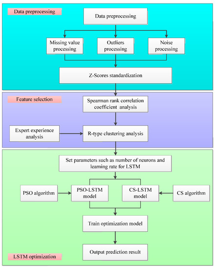
Figure 1. The framework of SIA-LSTM method.

In the data processing part, the missing value processing, outlier processing, noise processing, and Z-Scores standardization processing are carried out for the data of control parameters and related variables to remove the impact of different dimensions on the data.

In the feature selection part, Spearman’s rank correlation coefficient analysis and R-type clustering analysis are performed on the preprocessed variables. By calculating Spearman’s correlation coefficient and R-type clustering analysis results, feature selection is performed on the variables, successfully achieving the goal of dimensionality reduction.

In the optimization of LSTM using swarm intelligence algorithm part, the PSO algorithm and CS algorithm, which have a wide search range and fast convergence speed, are used to optimize some super parameters of LSTM. PSO-LSTM model and CS-LSTM model are constructed to find the optimal parameter set for LSTM, so as to better improve the prediction accuracy of the model.

Given the missing values, outliers, and noises in the data set, and different dimensions affecting the data analysis results, this paper conducts data preprocessing and Z-Scores standardization on the data set. Excessive variables can lead to a waste of computational resources and hinder the accuracy of prediction models, requiring feature selection. Many network parameters of the LSTM prediction model can affect the prediction accuracy of the LSTM model. However, these parameters are too dependent on empirical settings, resulting in unstable prediction accuracy. This problem is effectively solved by optimizing LSTM using PSO algorithm and CS algorithm.

2.1. Data Preprocessing

2.1.1. Missing Value Processing

Missing values are undesirable and unavoidable for statisticians and data collectors. Some statistical analysis methods are able to delete the observation record with a missing value directly. When there are fewer missing values, there will be no significant problems. However, when the number of missing values is large, a large amount of information will be lost directly and may lead to wrong conclusions, so a more systematic missing value analysis is needed.

A missing value has a certain regularity, and its missing mode can be roughly divided into the following three manners: missing completely at random, missing at random, and missing not at random. A large number of variables are involved in the process of data mining. When only one variable value is missing, the whole variable set should not be deleted. By describing and diagnosing the missing value, the severity of the missing value is evaluated. The correlation matrix, mean value, and covariance matrix with the missing value are estimated. The expected maximization method or regression algorithm is used to replace the missing values [22].

2.1.2. Outlier Processing

Outliers refer to the observed values that deviate from the whole sample population in the data set. The existence of outliers will reduce the normality of the data and the fitting ability of the model. In the process of data mining, these outliers need to be identified and processed. The detection methods of outliers mainly include cluster analysis, three sigma principle, simple statistics, boxplot method, and t test.

Cluster analysis is to group similar data observations into the same cluster. It mainly includes distance analysis method and density analysis method. Density analysis can discover clusters of any shape. The main idea of this method is that data in a certain region, as long as the density of data points is greater than the preset threshold value, will be divided into clusters similar to it, while data observations less than the threshold value are regarded as outliers. Outliers can be found by using this method [23].

2.1.3. Noise Processing

Noise data refer to the possible deviation or error of measured value relative to actual value when measuring variables. These data will affect the accuracy and effectiveness of subsequent analysis operations. Noise points can be identified by using data smoothing techniques, regression analysis, cluster analysis, and box-splitting methods.

Data smoothing is used to eliminate noise in signals. Kalman filtering is one of the most widely used filtering methods [24]. It can estimate the state of the dynamic system from a series of data with measurement noise, and predict the information of the current state of the system according to the previous state of the system, as shown in Equations (1) and (2).

$$y_L\left(l|l-1\right)=E_L\times y_L\left(l-1|l-1\right)+A_L\times v_L\left(l\right)+w_L\left(l\right)$$

(1)

$$H_L\left(l|l-1\right)=E_L\times H_L\left(l-1|l-1\right)\times E_L^{\prime }+P_L$$

(2)

Among them, y_L(l|l − 1) is the predicted value of the current state of the system; y_L(l − 1|l − 1) is the optimal value in the previous state of the system; H_L(l|l − 1) is the covariance corresponding to state y_L(l|l − 1); H_L(l − 1|l − 1) is the covariance corresponding to y_L(l − 1|l − 1); w_L(l) is the process noise, and its covariance is P_L; v_L(l) is the control variable of the current state; A_L is the control input matrix; E_L is the state transition matrix.

Through the current state composed of the system-predicted values and measured values C_L(l), the optimal estimate of the current state of the system T_L(l|l) is calculated, as shown in Equation (3).

$$T_L\left(l|l\right)=T_L\left(l|l-1\right)+B_L\left(l\right)\times \left(C_L\left(l\right)-D_L\times T_L\left(l|l-1\right)\right)$$

(3)

Among them, C_L(l) is the measured value of the system, and C_L(l) = D_L × y_L + u_L(l); D_L is the observation matrix; u_L is the observation noise, and its covariance is S_L; J_L(l) is the Kalman gain, as shown in Equation (4).

$$J_L\left(l\right)=\left(H_L\left(l|l-1\right)\times D_L^{\prime }\right)/\left(D_L\times H_L\left(l|l-1\right)\times D_L^{\prime }+S_L\right)$$

(4)

The covariance of the optimal estimated value under the updated state l is shown in Equation (5).

$$H_L\left(l|l-1\right)=\left(I_L-J_L\left(l\right)\right)\times H_L\left(l-1|l-1\right)$$

(5)

In the case of a single model and single measurement, I_L = 1. When the system is in the l + 1 state, H_L(l|l − 1) is the H_L(l − 1|l − 1) in Equation (2) [25].

2.1.4. Standardized Processing

Differences in order of magnitude can lead to larger orders of magnitude occupying a dominant position and slow iteration convergence speed. Therefore, it is necessary to preprocess the data to eliminate effects with different dimensions. The standardization of data processing involves converting the original data into a small specific interval, such as 0–1 or −1 to 1, through certain mathematical transformations to eliminate differences in the properties, orders of magnitude, and dimensions, making it easy to comprehensively analyze and compare indicators of different units or orders of magnitude. Z-Scores standardization is used to eliminate the influence of dimensions, as shown in Equation (6) [26].

$$x_{ij}^{*}=\left\{\begin{array}{c}\frac{x_{ij}-\overline{x_j}}{S_j} S_j\ne 0\\ \\ 0 S_j=0 \end{array}\right. \left(\begin{array}{c}i=1,2,\cdots ,n\\ j=1,2,\cdots ,n\end{array}\right)$$

(6)

where S_j is the standard deviation of the data, ${\overline{x}}_j$ is the mean of the data.

2.2. Feature Selection

According to the experience of experts, a feature selection method based on correlation analysis and R-type clustering analysis is proposed, which can effectively solve the problem of low correlation of some closely related variables in industrial production.

2.2.1. Spearman’s Rank Correlation Coefficient Analysis

Correlation analysis is to explore the degree and direction of correlation between variables with specific similar relationships, and to study whether there is a certain similar relationship between variables. The study of correlation analysis mainly focuses on the degree of closeness between two variables, which is a statistical method to study random variables. Correlation analysis studies the relationships and properties between variables. It is the fundamental work before data mining.

In feature selection methods, the Pearson or Spearman rank correlation coefficient is often used to quantify the dependence and monotonicity between two sets of data. The Pearson correlation coefficient is shown in Equation (7) [27].

$$r=\frac{{{\displaystyle \sum }}_{i=1}^n\left(x_i-\overline{x}\right)\left(y_i-\overline{y}\right)}{\sqrt{{{\displaystyle \sum }}_{i=1}^n{\left(x_i-\overline{x}\right)}^2}\sqrt{{{\displaystyle \sum }}_{i=1}^n{\left(y_i-\overline{y}\right)}^2}}$$

(7)

where $x_i$ and $y_i$ are the variable values, $n$ is the sample size.

The value of the Pearson correlation coefficient mainly depends on the size and degree distribution of the network. Especially for large-scale networks, it will converge to zero, which seriously hinders the quantitative comparison of different networks. Spearman’s rank correlation coefficient is a non-parametric measure, which is used when the data show an abnormal distribution between two variables. It is defined as the Pearson correlation coefficient between two rank random variables, recording the difference between the positive rank and the negative rank of each data point. For data samples with a sample size of n, x_i, and y_i are sorted from small to large and converted into rgx_i and rgy_i, where rgx_i and rgy_i are the ranks of x_i and y_i. If the rank after arrangement is the same, the Pearson correlation coefficient is calculated according to Equation (7). Otherwise, r is calculated according to Equation (8). The value ranges from −1 to 1.

$$r=1-\frac{6\sum d_i^2}{n\left(n^2-1\right)}$$

(8)

where d_i is the rank difference between x_i and y_i.

2.2.2. R-Type Clustering Analysis

R-type system clustering analysis uses the average inter-group distance method to cluster variables with high similarity, reducing variable dimensions and making data analysis easier [28]. The flowchart of the R-type clustering method is shown in Figure 2.

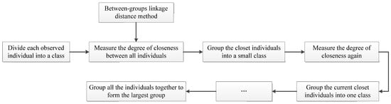
Figure 2. The flow chart of R-type clustering method.

2.3. LSTM Model

The main characteristics of LSTM neural network include the use of gate mechanism to improve the problem of recurrent neural network (RNN) being unable to transmit historical information for a long time, solve the problem of gradient vanishing and exploding during long sequence training, and achieve long-term time series learning [29]. It consists of input gate, output gate, and forgetting gate, which can selectively learn input information and store valuable information in memory units [30]. LSTM is widely used in various fields such as unmanned driving, intelligent robots, speech recognition, and other fields. The structure of LSTM is shown in Figure 3.

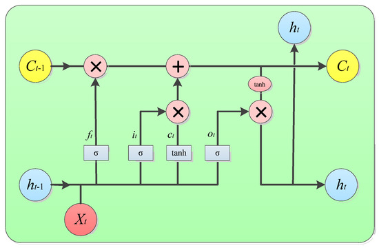
Figure 3. Structure diagram of LSTM neural network.

In Figure 3, c_t is the cell status update value at time t; h_t−1 and h_t respectively represent the output at time t − 1 and time t; C_t−1 and C_t respectively represent the cell state at time t − 1 and t; X_t is the input at time t; o_t, i_t and f_t represent output gate, input gate, and forgetting gate, respectively; o_t, i_t and f_t are all matrices with the element value range of [0, 1]; tanh and σ are activation functions. Equations (9)–(15) show the information transmission process of LSTM neural network.

$$tanh\left(x\right)=\frac{sinh\left(x\right)}{cosh\left(x\right)}$$

(9)

$$\sigma \left(x\right)=\frac{1}{1+e^{-x}}$$

(10)

$$h_t=o_t\times tanh\left(C_t\right)$$

(11)

$$C_t=f_t\times C_{t-1}+i_t\times c_t$$

(12)

$$f_t=\sigma \left(w_f·\left[h_{t-1},X_t\right]+b_f\right)$$

(13)

$$i_t=\sigma \left(w_i·\left[h_{t-1},X_t\right]+b_i\right)$$

(14)

$$o_t=\sigma \left(w_o·\left[h_{t-1},X_t\right]+b_0\right)$$

(15)

Among them, w_o, w_i, and w_f respectively represent the weight matrix of the three gates; b_o, b_i, and b_f respectively represent the bias terms of the three gates; σ is sigmoid function, which is an S-type function that can map the output results of real numbers within the [0, 1] interval. The value range of the tanh function is (−1, 1) [31].

Based on the above LSTM structure diagram and derived equations, the input of the LSTM neural network at time t is determined by the input X_t at the current time and the output h_t−1 at time t − 1. The cell status update value c_t at time t is determined by the input gate i_t, which is used to select useful information to update the unit state C_t. The forgetting gate f_t is used to control the cell state at t − 1 time and filter storage information. The joint effect of input gate i_t and forgetting gate f_t is to forget worthless information and update useful information to obtain the unit state C_t at time t. The output gate o_t is used to control the cell state C_t at time t. Firstly, the tanh function is used to map the value of the cell state C_t to the (−1, 1) interval, and then the input gate o_t is used to analyze the output h_t at time t.

2.4. Optimization of LSTM Prediction Model by Particle Swarm Optimization

The PSO algorithm can be described as that every bird in the population is a possible solution to the problem to be optimized, and it is called “particle”. All particles will be evaluated using fitness values determined by a function to be optimized [32]. PSO first initializes the state of the particles, obtaining a set of random parameter information. Then, the particles continuously update their positions through the use of local optimal solutions (P_best) and global optimal solutions (G_best) during continuous motion, and obtain the optimal parameter set after iteration. P_best and G_best respectively represent the optimal position of the particle fitness value of the whole population in the iteration process of spatial position. In the process of iteration, its speed and position are updated by Equations (16) and (17).

$$s_{kd}^{\left(l+1\right)}=g_c·s_{kd}^{\left(l\right)}+e_1·f_1·\left(h_{kd}^{\left(l\right)}-a_{kd}^{\left(l\right)}\right)+e_2·f_2·\left(h_{kd}^{\left(l\right)}-a_{kd}^{\left(l\right)}\right)$$

(16)

$$a_{kd}^{\left(l+1\right)}=a_{kd}^{\left(l\right)}+s_{kd}^{\left(l+1\right)}$$

(17)

Among them, $a_{kd}^{\left(l\right)}$ is the current position vector of the particle; $h_{kd}^{\left(l\right)}$ is the optimal position for individual particles; $s_{kd}^{\left(l\right)}$ is the velocity vector of particle motion; f₁ and f₂ are random numbers between (0,1); e₁ and e₂ are the acceleration factors of particles; g_c is the inertia factor [33].

The LSTM prediction model contains many network parameters, such as kernel function, learning rate, number of neurons, etc., which will affect the prediction accuracy of the LSTM model. Because these parameters are too dependent on the empirical setting, their prediction accuracy is unstable. At the same time, with the different parameter settings, the length of training time of LSTM model will also change [34]. The problem of selecting parameters manually can be solved by using particle swarm optimization algorithm to search some network parameters of LSTM model [35]. Aiming at the problems such as low accuracy and weak generalization ability of the model caused by manual parameter settings, this paper uses the PSO algorithm with a wide search range and fast convergence speed to optimize some super parameters of LSTM, build the PSO-LSTM model, and find the optimal parameter set for LSTM, so as to better improve the model prediction accuracy. Figure 4 shows the flow chart of PSO-LSTM model.

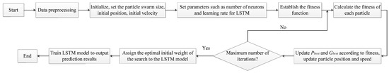
Figure 4. The flow chart of PSO-LSTM.

The specific steps of PSO-LSTM prediction model construction are as follows:

Step 1: Data preprocessing. The variable data are collected and the training set and testing set of the model are obtained through data preprocessing.

Step 2: Initialize parameters. Initialize the parameters of PSO, such as learning factor, number of iterations and particles, and so on. At the same time, the optimization range of LSTM parameters such as learning rate, time step, batch processing capacity, and number of hidden layer units is set.

Step 3: Evaluate particles. The mean values of MAE and RMSE between the real and predicted values of the test set in the LSTM model are taken as the particle fitness values. The obtained value is compared with the initial value P_best and G_best to obtain the optimal P_best and G_best.

Step 4: Update the position and velocity of the particles.

Step 5: Determine the termination condition. If the number of iterations reaches the preset value, stop searching and output the optimal parameter group. If not, return to Step 3 for iterative optimization.

After initializing the velocity and position of particles, PSO algorithm iteratively updates its position to obtain the optimal solution of the model. PSO algorithm has advantages such as good robustness and fast convergence speed for multi-dimensional space function optimization and multi-objective optimization, and is suitable for some hyperparameter optimization in neural networks, providing a theoretical basis for model combination. The PSO-LSTM prediction model optimized by particle swarm optimization algorithm achieves the best prediction effect by continuously iterating and searching for the optimal value of parameters within the given parameter range.

2.5. Optimization of LSTM Prediction Model by Cuckoo Algorithm

Cuckoo search algorithm is a simulation of the parasitic reproduction behavior of cuckoo birds during their breeding period. Cuckoo nests that lay eggs by means of parasitic brood rearing are a solution to the optimization problem, which needs to be updated by cuckoos’ flight. The process of cuckoos’ nest search represents the updated operation of solution. Cuckoo birds use unique Lévy flights and random walks to find new nests [36].

The CS algorithm is based on the following rules:

Rule 1: Each cuckoo lays only one egg at a time, and a nest is randomly selected for hatch;

Rule 2: From randomly selected bird nests, the nest with the best quality eggs is reserved for the next generation;

Rule 3: The number of nests is fixed, the probability that the original owner found the alien eggs is P_a, and P_a ∈ [0, 1]. When the original owner finds the eggs, they will throw them away or abandon the nest, and find another place to rebuild the nest [37].

Aiming at problems such as low accuracy and weak generalization ability of the LSTM model caused by manual parameter settings, this section adopts CS algorithm with good global and local search ability and fast convergence speed to optimize some super parameters of LSTM, build CS-LSTM model, and find the optimal parameter set for LSTM, so as to better improve the prediction accuracy of the model. Figure 5 shows the flow chart of CS-LSTM model.

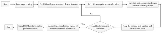
Figure 5. The flow chart of CS-LSTM.

The specific steps of CS-LSTM prediction model construction are as follows:

Step 1: Data preprocessing. Collect variable data and obtain the training and testing sets of the model through data preprocessing.

Step 2: Initialize parameters. Initialize the parameters of CS, such as learning factor, iteration number, and so on. At the same time, the optimization range of LSTM parameters such as learning rate, time step, batch processing capacity, and number of hidden layer units is set.

Step 3: Set the dimension D of the solution of the actual problem. The maximum number of iterations is L; Cuckoo population size N in the algorithm; C The probability of a cuckoo bird’s egg being discovered is f_a. By randomly generating n cuckoo nest locations, $p_i^{\left(t\right)}$, i = 1, 2, …, n, calculate the fitness value, and determine and save the current optimal nest location G_best.

Step 4: Update the current nest position, calculate and compare the fitness values of the child nest and the parent nest, and save the nest position with better fitness value to the next generation, $p_i^{\left(t\right)}$, i = 1, 2, …, n.

Step 5: Compare the value of the optimal fitness function of the previous generation and update the position G_best of the optimal solution of this generation. Judge whether the algorithm meets the convergence condition. If it meets the convergence condition, output the optimal position G_best; otherwise, jump back to Step 4 and repeat the optimization iteration until L iterations are completed [38].

Step 6: Determine the termination condition. If met, then stop the search, and output the optimal parameter set. If not, then return for iterative optimization.

2.6. Predictive Performance Evaluation Index

This paper mainly selects four indicators as the model evaluation indicators, namely, determination coefficient, mean absolute error, root mean square error, and mean absolute percentage error, so as to evaluate the prediction effect of the model more comprehensively and accurately. The calculation formula is as follows:

(1)

Determination coefficient

R² is the coefficient of determination, which measures how well the predicted value fits the real value. R² ranges from (0 to 1), and the closer it is to 1, the better model fitting is.

(2)

Mean absolute error

The mean absolute error can be obtained by directly calculating the mean value of the residual error, which represents the mean value of the absolute error between the predicted and observed values. The mean absolute error is a linear fraction in which all observed individual differences are weighted over the mean. The calculation formula is shown in Equation (18).

$$MAE=\frac{1}{n}{\displaystyle \sum }_{i=1}^n\left|p_i-r_i\right|$$

(18)

(3)

Root mean square error

The root mean square error is the square root of the expected value of the difference between the estimated value and the true value of the data. The root mean square error refers to the sum of the squares of the distances between each data deviation from the true value, which is then averaged and squared. The smaller the index, the higher the accuracy. The calculation formula is shown in Equation (19).

$$RMSE=\sqrt{\frac{1}{n}{\displaystyle \sum }_{i=1}^n{\left(p_i-r_i\right)}^2}$$

(19)

(4)

Mean absolute percentage error

The mean absolute percentage error is the percentage value, that is, the expected value of the relative error loss, which is the percentage of the absolute error and the true value. In model prediction, the smaller the mean absolute percentage error, the better the accuracy of the model. The calculation formula is shown in Equation (20).

$$MAPE=\frac{100}{n}{\displaystyle \sum }_{i=1}^n\left|\frac{r_i-p_i}{r_i}\right|$$

(20)

Among them, n is the number of samples; r_i is the actual value; p_i is the predicted value.

3. Industrial Applications

3.1. Process Description

The case in this paper comes from a catalytic cracking unit of a petrochemical enterprise. Over two years, 347,520 observations are collected every 3 min. The collection time of all variables in the device is the same. Figure 6 shows the process of the catalytic cracking unit [26]. It mainly consists of R-1 reactor, R-2 regenerator, B-1 raw material buffer tank, C-1 fractionation column, C-2 diesel stripper, C-3 absorption column, C-4 desorption column, C-5 stabilization column, and C-6 reabsorption column. S-1 is the buffer tank. B-2 is the oil and gas separator at the top of the fractionation tower. B-3 is the top return tank of the absorption tower. B-4 is the stabilizer top return tank. P-1, P-2, …, P-8 are pumps. E-1, E-2, …, E-6 are heating devices. The output includes OUTPUT1 light diesel, OUTPUT2 liquefied gas, OUTPUT3 stable gas, OUTPUT4 dry gas, and OUTPUT5 rich absorption oil.

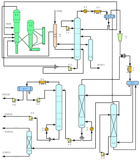
Figure 6. The flow chart of the catalytic cracking unit.

The training set and test set of the LSTM model, PSO-LSTM model, and CS-LSTM model are constructed by the main control variables. The test set is predicted by learning the complex relationships between the variables of the training set and their long-term sequence memory. In the prediction of the main control variable, the variable after feature selection is selected as the input variable, and the main control variable is the prediction variable. In this paper, representative cases of reaction temperature (TIC1001) prediction and liquid level at the bottom of the fractionator (LIC2001) prediction are selected for an explanation.

As one of the main control parameters of the catalytic cracking process, the reaction temperature can have a significant impact on the depth of the reaction, which can change the quality and yield of the product. The liquid level at the bottom of the fractionating column is an important parameter for the whole column operation. The change in liquid level at the bottom of the column reflects the state of material balance and heat balance of the whole column, which has a significant impact on the operation of the entire column.

3.2. Data Preprocessing of Main Control Variables

When a few variables in the data set have missing values, the missing values are replaced by the expectation maximization method. The Kalman filtering method is used to smooth the data and Z-Scores standardization is carried out on all variables to eliminate the effect of different dimensionality. The standard deviation of the converted data is one and the mean is zero.

3.3. Feature Selection of TIC1001 and LIC2001

After communicating with field experts, and comprehensively considering mechanism analysis, process principles, and practical working experience, 20 variables related to reaction temperature are selected [16,39]. There are many variables in the catalytic cracking process; however, excessive variables can make data analysis more difficult. Only variables related to TIC1001 are considered. The Spearman rank correlation values between TIC1001 and its related variables are shown in Table 1, and the R-type clustering results between TIC1001 and its related variables are shown in Figure 7.

Table 1. Main variables related to TIC1001.

Variable Tag Number	Variable Description	The Spearman Rank Correlation Coefficient Value with TIC1001
TIC1001	Reaction temperature	1.000
FI2065	Riser feed rate	0.131
FIC2014	Flow rate of oil slurry entering the fractionator (back under the column)	0.289
PDIC1002	Regenerative inclined tube slide valve pressure drop	0.283
FIC1002	Flow of riser oil recycled slurry	0.148
FIC1035	Quench water entering the riser	−0.185
FIC2004	Flow of reflux oil entering the fractionator	0.138
FIC2013	Flow rate of oil slurry entering the fractionator (back on the column)	0.352
ZSQSJF	Coke discharge amount	0.006
PI1056	Reaction pressure	0.238
PIC1011	Regeneration pressure	0.248
FIC1027	Flow of burning oil to coking tank	0.033
TIC2006	Raw material preheating temperature	0.168
LZI1002	Circulating inclined pipe slide valve position	0.054
TZI1001	Valve position of the regenerated catalyst slide valve	0.160
FIC1006	Riser pre-lift steam volume	0.274
FIQ2062	Flue gas oxygen content	0.155
LIC1003	Reactor stripping section control material level	0.216
AI1001	Oxygen content in flue gas	−0.084
LZI1003	Waiting spool valve position	0.272

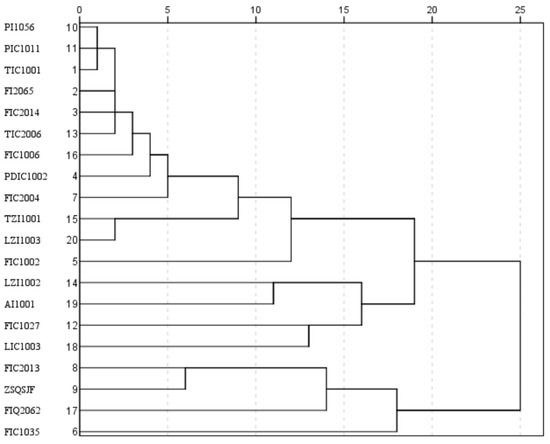
Figure 7. R-type clustering results of main variables related to TIC1001.

The Spearman rank correlation coefficient values between TIC1001 and its related variables in Table 1 and the R-type clustering results between TIC1001 and its related variables in Figure 7 intuitively reflect the relationship between reaction temperature and its related variables. The vertical axis in Figure 7 shows the clustering order between variables, and the horizontal axis shows that these variables can be divided into several categories when given different distances. Based on the Spearman rank correlation coefficient values between TIC1001 and its related variables, R-type clustering results between TIC1001 and its related variables, and expert experience, 12 variables are obtained through feature selection, as shown in Table 2. Through feature selection, the dimensionality of data variables is effectively reduced.

Table 2. After feature selection main variables related to TIC1001.

Variable Tag Number	Variable Description	The Spearman Rank Correlation Coefficient Value with TIC1001
TIC1001	Reaction temperature	1.000
FIC1035	Quench water entering the riser	−0.185
FIC2013	Flow rate of oil slurry entering the fractionator (back on the column)	0.352
FIC2014	Flow rate of oil slurry entering the fractionator (back under the column)	0.289
PDIC1002	Regenerative inclined tube slide valve pressure drop	0.283
PI1056	Reaction pressure	0.238
PIC1011	Regeneration pressure	0.248
TIC2006	Raw material preheating temperature	0.168
TZI1001	Regenerative spool valve position	0.160
FIC1006	Riser pre-lift steam volume	0.274
LIC1003	Reactor stripping section control material level	0.216
LZI1003	Waiting spool valve position	0.272

After communicating with field experts, and comprehensively considering mechanism analysis, process principles, and practical working experience, 19 variables related to the liquid level at the bottom of the fractionator are selected. The Spearman rank correlation values between LIC2001 and its related variables are shown in Table 3, and the R-type clustering results between LIC2001 and its related variables are shown in Figure 8.

Table 3. Main variables related to LIC2001.

Variable Tag Number	Variable Description	The Spearman Rank Correlation Coefficient Value with LIC2001
LIC2001	Liquid level at the bottom of the fractionator	1.000
FIC1002	Flow of riser oil recycled slurry	0.132
FIC2013	Flow rate of oil slurry entering the fractionator (back on the column)	−0.057
FIC2014	Flow rate of oil slurry entering the fractionator (back under the column)	−0.010
FIC2015	Oil slurry flow back to the column	0.080
FIC2029	Stirring steam at the bottom of the fractionator	0.328
FIC2027	Steam stripping capacity of diesel column	0.010
FIC2016	Oil slurry outflow	0.134
LIC2019	Liquid level of crude steam tank	0.239
LIC3011	Liquid level of oil gas separator at the outlet of the gas compressor	0.132
FIC3018	Flow rate of condensed oil returning to the fractionator	−0.094
PI2052	Top pressure of fractionating column	0.086
TI2064	Bottom temperature of fractionating column	0.121
LIC3012	Boundary position of oil gas separator at the outlet of the gas compressor	0.056
TIC2011	Temperature of returning oil to the fractionation column	0.129
TIC2004	Top temperature of fractionating column	0.098
FIC2011	Light diesel outlet flow rate	−0.046
FI2076	Recycle water in reaction-regeneration and fractionation zones	0.331
TIC2065	Inlet temperature of aftercooler at top of fractionating column	−0.072

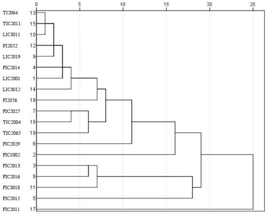
Figure 8. R-type clustering results of main variables related to LIC2001.

The Spearman rank correlation coefficient values between LIC2001 and its related variables in Table 3 and the R-type clustering results between LIC2001 and its related variables in Figure 8 intuitively reflect the relationship between the liquid level at the bottom of the fractionator and its related variables. The vertical axis in Figure 8 shows the clustering order between variables, and the horizontal axis shows that these variables can be divided into several categories when given different distances. Based on the Spearman rank correlation coefficient values between LIC2001 and its related variables, R-type clustering results between LIC2001 and its related variables, and expert experience, 12 variables are obtained through feature selection, as shown in Table 4.

Table 4. After feature selection main variables related to LIC2001.

Variable Tag Number	Variable Description	The Spearman Rank Correlation Coefficient Value with LIC2001
LIC2001	Liquid level at the bottom of the fractionator	1.000
FI2076	Recycle water in reaction–regeneration and fractionation zones	0.331
FIC1002	Flow of riser oil recycled slurry	0.132
FIC2015	Oil slurry flow back to the column	0.080
FIC2029	Stirring steam at the bottom of the fractionator	0.328
FIC2016	Oil slurry outflow	0.134
LIC2019	Liquid level of crude steam tank	0.239
LIC3011	Liquid level of oil gas separator at the outlet of the gas compressor	0.132
PI2052	Top pressure of fractionating column	0.086
TI2064	Bottom temperature of fractionating column	0.121
TIC2011	Temperature of returning oil to the fractionation column	0.129
TIC2004	Top temperature of fractionating column	0.098

3.4. Prediction Cases of TIC1001 and LIC2001

In the prediction of the main control variable reaction temperature, 11 variables after feature selection are selected as input variables, as shown in Table 2. In the prediction, 2400 continuous time series data are selected, including 2000 data for the training set and 400 data for the testing set. The prediction results of the TIC1001 training set and testing set are shown in Figure 9 and Figure 10, respectively. TIC1001 temperature control is in the normal range of 500~530 °C. The real value and model predicted value of TIC1001 in part of the testing set are given in Table 5. The evaluation of the prediction results under different indicators of TIC1001 is shown in Table 6.

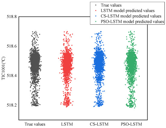
Figure 9. TIC1001 predicted results of training set.

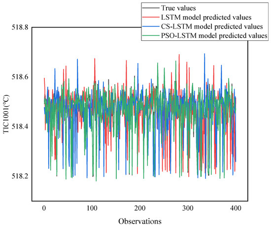
Figure 10. TIC1001 predicted results of testing set.

Table 5. The real value and model predicted value of TIC1001.

Serial Number	True Value	LSTM Predicted Value	CS-LSTM Predicted Value	PSO-LSTM Predicted Value
1	518.4715	518.4719	518.4663	518.47864
2	518.48592	518.4889	518.52124	518.47784
3	518.52107	518.5277	518.52972	518.5116
4	518.54446	518.4467	518.44537	518.53778
5	518.47006	518.4611	518.47433	518.47382
6	518.34621	518.3352	518.33233	518.33148
7	518.51147	518.5091	518.48543	518.50787
8	518.51864	518.5393	518.53835	518.53748
9	518.44836	518.4701	518.46449	518.46399
10	518.51106	518.51162	518.51159	518.51453
11	518.51893	518.51366	518.51106	518.51447
12	518.63592	518.6215	518.62973	518.63531
13	518.53461	518.54041	518.55927	518.55499
14	518.45267	518.455991	518.45023	518.44873
15	518.34756	518.34983	518.33497	518.34521
16	518.49772	518.50447	518.48826	518.50415
17	518.47403	518.47928	518.47861	518.47754
18	518.45139	518.45863	518.46292	518.43738
19	518.43175	518.4392	518.43299	518.43323
20	518.49549	518.49602	518.49654	518.49078
21	518.46788	518.4635	518.46619	518.46613
22	518.44101	518.45896	518.45237	518.45972
23	518.52609	518.22284	518.52621	518.52869
24	518.53516	518.52293	518.53354	518.52106
25	518.49449	518.49096	518.49106	518.49304
26	518.54595	518.54837	518.54469	518.54761
27	518.49366	518.4978	518.49191	518.50014
28	518.4342	518.43156	518.4324	518.42725
29	518.47716	518.458026	518.47475	518.47064
30	518.52508	518.52144	518.52146	518.52246

Table 6. Evaluation of prediction results for different indicators of TIC1001.

Model	LSTM	CS-LSTM	PSO-LSTM
R2	0.9554	0.9836	0.9867
MAE	0.0147	0.0087	0.0081
RMSE	0.0186	0.0110	0.0104
MAPE	0.0028%	0.0017%	0.0016%

As shown in Figure 9, Figure 10, and Table 6, TIC1001 achieves good prediction results in both the training and testing sets of the PSO-LSTM model and the CS-LSTM model. The predicted value curve of the PSO-LSTM model is close to the true value, with the R² value of 0.9867, MAE value of 0.0081, RMSE value of 0.0104, and MAPE value of 0.0016%. The R² index of the PSO-LSTM model increased by 3.17%, the MAE decreased by 44.90%, the RMSE decreased by 44.09%, and the MAPE decreased by 42.86%, achieving good model prediction results. The predicted value curve of the CS-LSTM model is also close to the true value, with the R² value of 0.9836, MAE value of 0.0087, RMSE value of 0.0110, and MAPE value of 0.0017%. The R² index of the CS-LSTM model increased by 2.95%, the MAE decreased by 40.82%, the RMSE decreased by 40.86%, and the MAPE decreased by 39.29%, achieving good model prediction results. In the comparison of prediction results among different models, it can be seen that the PSO-LSTM model has relatively better prediction results and smaller errors.

In the prediction of the main control variable liquid level at the bottom of the fractionator, 11 variables after feature selection are selected as input variables, as shown in Table 4. In the prediction, 2400 continuous time series data are selected, including 2000 data for the training set and 400 data for the testing set. The prediction results of the LIC2001 training set and testing set are shown in Figure 11 and Figure 12, respectively. The liquid level of LIC2001 is controlled in the normal range of 40~80%. The real value and model predicted value of LIC2001 in part of the testing set are given in Table 7. The evaluation of the prediction results under different indicators of LIC2001 is shown in Table 8.

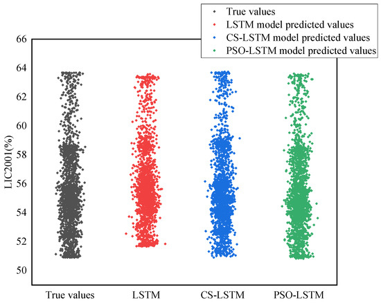
Figure 11. LIC2001 predicted results of training set.

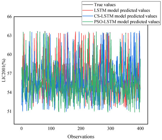
Figure 12. LIC2001 predicted results of testing set.

Table 7. The real value and model predicted value of LIC2001.

Serial Number	True Value	LSTM Predicted Value	CS-LSTM Predicted Value	PSO-LSTM Predicted Value
1	51.77899	51.8564	51.648031	52.011272
2	54.42288	54.19416	54.276474	54.370945
3	55.83517	55.75066	55.898516	55.892471
4	51.06081	51.36805	51.346381	51.283443
5	58.54155	58.54901	58.494977	58.5271
6	55.622	56.65013	56.627747	56.147087
7	58.37823	58.80294	58.732814	58.726921
8	50.90714	51.36358	51.272394	51.258907
9	55.59414	55.4164	55.439137	55.931633
10	53.43696	53.33577	53.330453	53.332516
11	54.915	54.9453	54.165844	55.125683
12	57.81279	58.5052	58.97047	58.566498
13	54.87991	55.40459	55.68013	55.324322
14	62.65866	63.42329	63.511147	63.100113
15	59.06907	59.22119	59.732464	59.053585
16	55.23773	55.55943	55.737644	55.512531
17	51.0186	51.33752	51.415874	51.292053
18	55.90675	56.83082	56.073032	56.31971
19	60.75861	60.20554	60.223503	60.835606
20	63.23134	63.87065	63.75391	63.45153
21	50.98838	52.85928	52.117191	51.537224
22	63.10177	63.40903	63.266612	63.344803
23	52.47703	52.78905	52.090408	52.989368
24	61.91469	61.70058	62.762131	62.360985
25	57.05719	57.95876	57.159863	57.101185
26	54.73388	54.75581	54.753345	54.747967
27	54.84255	54.829076	54.82662	54.836576
28	55.17831	55.235021	55.20784	55.181977
29	54.57612	54.511195	54.55252	54.446237
30	54.4342	54.03102	54.54358	54.533562

Table 8. Evaluation of prediction results for different indicators of LIC2001.

Model	LSTM	CS-LSTM	PSO-LSTM
R2	0.9637	0.9887	0.9945
MAE	0.4733	0.2533	0.1386
RMSE	0.5585	0.3115	0.1220
MAPE	0.8368%	0.4523%	0.2491%

As shown in Figure 11, Figure 12, and Table 8, LIC2001 achieves good prediction results in both the training and testing sets of the PSO-LSTM model and the CS-LSTM model. The predicted value curve of the PSO-LSTM model is close to the true value, with the R² value of 0.9945, MAE value of 0.1386, RMSE value of 0.1220, and MAPE value of 0.2491%. The R² index of the PSO-LSTM model increased by 3.20%, the MAE decreased by 70.72%, the RMSE decreased by 78.16%, and the MAPE decreased by 70.23%, achieving good model prediction results. The predicted value curve of the CS-LSTM model is also close to the true value, with the R² value of 0.9887, MAE value of 0.2533, RMSE value of 0.3115, and MAPE value of 0.4523%. The R² index of the CS-LSTM model increased by 2.60%, the MAE decreased by 46.48%, the RMSE decreased by 44.23%, and the MAPE decreased by 45.95%, achieving good model prediction results. In the comparison of prediction results among different models, it can be seen that the PSO-LSTM model has better prediction results and smaller errors.

In comparison with the research results of related research literature, the multiple-level LSTM (ML-LSTM) was used to predict the yield of FCC gasoline [15]. The RMSE and R² values of the ML-LSTM model are 0.5851 and 0.4384, respectively. The results of R² and RMSE in this paper are better. In the AHMPSO-AM-LSTM model, to predict the chemical oxygen demand of key characteristics in the wastewater treatment plant, the RMSE decreased by 7.803–19.499%, MAE decreased by 9.669–27.551%, MAPE decreased by 8.993–25.996%, and R² increased by 3.313–11.229% [20]. In contrast, the RMSE, MAE, and MAPE of the model in this paper are reduced more.

4. Conclusions

In this paper, the missing value processing, outlier processing, noise processing, and Z-Scores standardization processing are carried out for the data of control parameters and related variables to remove the impact of different dimensions on the data. Twelve variables related to TIC1001 and 12 variables related to LIC2001 are obtained. A novel SIA-LSTM method is proposed. The PSO-LSTM model and CS-LSTM model are constructed by using the PSO algorithm and CS algorithm with a wide search range and fast convergence speed to optimize some LSTM super parameters. Compared with the prediction results of the LSTM model, R², RMSE, MAE, and MAPE indexes of the PSO-LSTM model and CS-LSTM model show excellent prediction performance. In the prediction of reaction temperature, the R² index of the PSO-LSTM model increased by 3.17%, the MAE decreased by 44.90%, the RMSE decreased by 44.09%, and the MAPE decreased by 42.86%. The R² index of the CS-LSTM model increased by 2.95%, the MAE decreased by 40.82%, the RMSE decreased by 40.86%, and the MAPE decreased by 39.29%. In the prediction of the liquid level at the bottom of the fractionator, the R² index of the PSO-LSTM model increased by 3.20%, the MAE decreased by 70.72%, the RMSE decreased by 78.16%, and the MAPE decreased by 70.23%. The R² index of the CS-LSTM model increased by 2.60%, the MAE decreased by 46.48%, the RMSE decreased by 44.23%, and the MAPE decreased by 45.95%. Both the PSO-LSTM model and CS-LSTM model proposed in this paper have high accuracy and feasibility in predicting the main control variables of the catalytic cracking process.

The potential research directions in the future will include the further optimization and improvement of prediction algorithms to achieve rapid and effective identification and prediction of major control states in industrial production. Further research will be conducted to combine predictive models with early warning models to reduce the occurrence of safety accidents.

References

- Cui, Z.; Tian, W.; Wang, X.; Fan, C.; Guo, Q.; Xu, H. Safety integrity level analysis of fluid catalytic cracking fractionating system based on dynamic simulation. J. Taiwan Inst. Chem. Eng. 2019, 104, 16–26. [Google Scholar] [CrossRef]
- Huang, M.; Zheng, Y.; Li, S. Distributed economic model predictive control for an industrial fluid catalytic cracking unit ensuring safe operation. Control Eng. Pract. 2022, 126, 105263. [Google Scholar] [CrossRef]
- Xiong, S.; Zhou, L.; Dai, Y.; Ji, X. Attention-based long short-term memory fully convolutional network for chemical process fault diagnosis. Chin. J. Chem. Eng. 2023, 56, 1–14. [Google Scholar] [CrossRef]
- Agudelo, C.; Anglada, F.; Cucarella, E.; Moreno, E. Integration of techniques for early fault detection and diagnosis for improving process safety: Application to a Fluid Catalytic Cracking refinery process. J. Loss Prev. Process Ind. 2013, 26, 660–665. [Google Scholar] [CrossRef]
- Taira, G.R.; Park, S.W.; Zanin, A.C. Fault detection in a fluid catalytic cracking process using bayesian recurrent neural network. IFAC-PapersOnLine 2022, 55–57, 715–720. [Google Scholar] [CrossRef]
- Shah, P.; Choi, H.K.; Kwon, J.S.I. Achieving optimal paper properties: A layered multiscale kMC and LSTM-ANN-based control approach for kraft pulping. Processes 2023, 11, 809. [Google Scholar] [CrossRef]
- Kim, H.J.; Baek, S.W. Application of wearable gloves for assisted learning of sign language using artificial neural networks. Processes 2023, 11, 1065. [Google Scholar] [CrossRef]
- Li, H.; Zhao, W.; Shi, Y.; Li, J. MP-CRJ: Multi-parallel cycle reservoirs with jumps for industrial multivariate time series predictions. Trans. Inst. Meas. Control 2022, 44, 2093–2105. [Google Scholar] [CrossRef]
- Liu, L. Research of railway passenger volume forecast model based on PCA-BP neural network. Compr. Transp. 2016, 8, 43–47. [Google Scholar]
- Tao, L.; Tian, G.; Aberer, K. Hybrid neural networks for learning the trend in time series. In Proceedings of the 26th International Joint Conference on Artificial Intelligence, Melbourne, Australia, 19–25 August 2017; pp. 2273–2279. [Google Scholar]
- Chen, Y.; Yu, W. A forecasting model of financial market index based on sparse autoencoder. J. Appl. Stat. Manag. 2021, 40, 93–104. [Google Scholar]
- Sun, H.; Wei, X. Research on stock index futures forecast based on trend learning and hybrid neural network. China J. Econom. 2021, 1, 921–934. [Google Scholar]
- Deng, X.; Wan, L.; Huang, N. Stock Prediction Research Based on DAE-BP Neural Network. Comput. Eng. Appl. 2019, 55, 126–132. [Google Scholar]
- Guo, J.; Wang, W.; Tang, Y.; Zhang, Y.; Zhuge, H. A CNN-Bi_LSTM parallel network approach for train travel time prediction. Knowl.-Based Syst. 2022, 256, 109796. [Google Scholar] [CrossRef]
- Yang, F.; Sang, Y.; Lv, J.; Cao, J. Prediction of gasoline yield in fluid catalytic cracking based on multiple level LSTM. Chem. Eng. Res. Des. 2022, 185, 119–129. [Google Scholar] [CrossRef]
- Tian, W.; Wang, S.; Sun, S.; Li, C.; Lin, Y. Intelligent prediction and early warning of abnormal conditions for fluid catalytic cracking. Chem. Eng. Res. Des. 2022, 181, 304–320. [Google Scholar] [CrossRef]
- Yang, F.; Dai, C.; Tang, J.; Xuan, J.; Cao, J. A hybrid deep learning and mechanistic kinetics model for the prediction of fluid catalytic cracking performance. Chem. Eng. Res. Des. 2020, 155, 202–210. [Google Scholar] [CrossRef]
- Wu, C.; Wang, C.; Kim, J.W. Welding sequence optimization to reduce welding distortion based on coupled artificial neural network and swarm intelligence algorithm. Eng. Appl. Artif. Intell. 2022, 114, 1105142. [Google Scholar] [CrossRef]
- Hu, S.; Yin, H. Research on the optimum synchronous network search data extraction based on swarm intelligence algorithm. Future Gener. Comput. Syst. 2021, 125, 151–155. [Google Scholar] [CrossRef]
- Liu, X.; Shi, Q.; Liu, Z.; Yuan, J. Using LSTM Neural Network Based on Improved PSO and Attention Mechanism for Predicting the Effluent COD in a Wastewater Treatment Plant. IEEE Access 2021, 9, 146082–146096. [Google Scholar] [CrossRef]
- Xiao, M.; Liao, Y.; Bartos, P.; Filip, M.; Geng, G.; Jiang, Z. Fault diagnosis of rolling bearing based on back propagation neural network optimized by cuckoo search algorithm. Multimed. Tools Appl. 2022, 81, 1567–1587. [Google Scholar] [CrossRef]
- Luo, L.; Bao, S.; Peng, X. Robust monitoring of industrial processes using process data with outliers and missing values. Chemom. Intell. Lab. Syst. 2019, 192, 103827. [Google Scholar] [CrossRef]
- Wang, B.; Mao, Z. Outlier detection based on Gaussian process with application to industrial processes. Appl. Soft Comput. 2019, 76, 505–516. [Google Scholar] [CrossRef]
- Yang, F.; Yang, J. Multiband-structured Kalman filter. IET Signal Process. 2018, 12, 722–728. [Google Scholar] [CrossRef]
- Garcia, R.V.; Pardal, P.C.P.M.; Kuga, H.K.; Zanardi, M.C. Nonlinear filtering for sequential spacecraft attitude estimation with real data: Cubature Kalman Filter, Unscented Kalman Filter and Extended Kalman Filter. Adv. Space Res. 2019, 63, 78320–78344. [Google Scholar] [CrossRef]
- Hong, J.; Qu, J.; Tian, W.D.; Cui, Z.; Liu, Z.J.; Lin, Y.; Li, C.K. Identification of unknown abnormal conditions in catalytic cracking process based on two-step clustering analysis and signed directed graph. Processes 2021, 9, 2055. [Google Scholar] [CrossRef]
- Liu, N.; Wang, J.; Sun, S.L.; Li, C.K.; Tian, W.D. Optimized principal component analysis and multi-state Bayesian network integrated method for chemical process monitoring and variable state prediction. Chem. Eng. J. 2022, 430, 132617. [Google Scholar] [CrossRef]
- Xue, W. Statistical Analysis and SPSS Application; China Renmin University Press: Beijing, China, 2017; pp. 269–272. [Google Scholar]
- Hochreiter, S.; Schmidhuber, J. Long short-term memory. Neural Comput. 1997, 9, 1735–1780. [Google Scholar] [CrossRef]
- Shu, X.; Zhang, L.; Sun, Y.; Tang, J. Host–parasite: Graph LSTM-in-LSTM for group activity recognition. IEEE Trans. Neural Netw. Learn. Syst. 2021, 32, 663–674. [Google Scholar] [CrossRef]
- Zhang, Z.; Lv, Z.; Gan, C.; Zhu, Q. Human action recognition using convolutional LSTM and fully-connected LSTM with different attentions. Neurocomputing 2020, 410, 304–316. [Google Scholar] [CrossRef]
- Ang, K.M.; Lim, W.H.; Isa, N.; Tiang, S.; Wong, C. A constrained multi-swarm particle swarm optimization without velocity for constrained optimization problems. Expert Syst. Appl. 2020, 140, 112882. [Google Scholar] [CrossRef]
- Kassoul, K.; Zufferey, N.; Cheikhrouhou, N.; Belhaouari, S.B. Exponential Particle Swarm Optimization for Global Optimization. IEEE Access 2022, 10, 78320–78344. [Google Scholar] [CrossRef]
- Suebsombut, P.; Sekhari, A.; Sureephong, P.; Bouras, A. Field data forecasting using LSTM and Bi-LSTM approaches. Appl. Sci. 2021, 11, 11820. [Google Scholar] [CrossRef]
- Tsai, H.-C. Unified particle swarm delivers high efficiency to particle swarm optimization. Appl. Soft Comput. 2017, 55, 371–383. [Google Scholar] [CrossRef]
- Tang, H. Cuckoo search algorithm with different distribution strategy. Int. J. Bio-Inspired Comput. 2019, 13, 234–241. [Google Scholar] [CrossRef]
- Gao, S.; Gao, Y.; Zhang, Y.; Xu, L. Multi-Strategy Adaptive Cuckoo Search Algorithm. IEEE Access 2019, 7, 137642–137655. [Google Scholar] [CrossRef]
- Rajabioun, R. Cuckoo Optimization Algorithm. Appl. Soft Comput. 2011, 11, 5508–5518. [Google Scholar] [CrossRef]
- Wang, S.; Tian, W.; Li, C.; Cui, Z.; Liu, B. Mechanism-based deep learning for tray efficiency soft-sensing in distillation process. Reliab. Eng. Syst. Saf. 2023, 231, 109012. [Google Scholar] [CrossRef]
Disclaimer/Publisher’s Note: The statements, opinions and data contained in all publications are solely those of the individual author(s) and contributor(s) and not of MDPI and/or the editor(s). MDPI and/or the editor(s) disclaim responsibility for any injury to people or property resulting from any ideas, methods, instructions or products referred to in the content. |
© 2023 by the authors. Licensee MDPI, Basel, Switzerland. This article is an open access article distributed under the terms and conditions of the Creative Commons Attribution (CC BY) license (https://creativecommons.org/licenses/by/4.0/).