Abstract
In the position control of the mechanical arm of an iron roughneck (MAIR), a controller with high responsiveness, high accuracy, and high anti-interference capability is necessary. An MAIR consists of two proportional-valve-controlled single-extension (PVCSE) hydraulic cylinders, and a traditional proportional–integral–derivative (PID) controller cannot easily achieve the accuracy and robustness requirements of the hydraulic cylinders. In this paper, a three-dimensional fuzzy active disturbance rejection controller (TF-ADRC) is proposed for an MAIR, which adds a three-dimensional fuzzy module to a classical active disturbance rejection controller (ADRC) to adjust the controller output according to the tracking of differential deviation, deviation change rate, and deviation change acceleration rate. Firstly, the trajectory planning of the MAIR was carried out using the quintic polynomial interpolation method to improve the smoothness of the target trajectory. Then, the reliability of the established model was verified by experiments. Finally, the comprehensive performance of a PID controller, fuzzy PID controller, ADRC, and TF-ADRC were compared based on the AMESim-Simulink model. The system with the TF-ADRC exhibits higher position control accuracy and better anti-interference capability than the system with a PID or Fuzzy PID controller, and accuracy is higher compared with the common ADRC.
1. Introduction
An iron roughneck is a multi-functional, safe, and efficient drilling tool that mainly installs/uninstalls a drill pipe joint, dumps the drill pipe and moves downhole tools [1]. An iron roughneck mainly consists of an actuator and an electrohydraulic servo system. Its actuator mainly consists of a clamp head and mechanical arm. This study addresses the mechanical arm of an iron roughneck and its electrohydraulic servo system. Electrohydraulic servo systems have been widely used in many fields, such as the aerospace, robotics, and construction industries, because of their small size, light weight, fast response, and high accuracy [2,3]. Hydraulic position control systems are widely used in hydraulic actuators as one of the electrohydraulic servo systems [4,5]. Current research on iron roughnecks mainly focuses on the design of actuators and neglects the electro-hydraulic servo systems. Iron roughnecks usually work under high load conditions and require high accuracy; therefore, electrohydraulic proportional position control systems are well suited for iron roughnecks.
Iron roughnecks are a kind of hydraulic robot arm. Trajectory planning can make them run more smoothly. The current methods of trajectory planning mainly include cubic polynomial interpolation and quintic polynomial interpolation. For velocity-limited industrial robot point-to-point joint motion planning, cubic polynomial planning has the problem of discontinuous acceleration, while quintic polynomial interpolation can realize the smooth transition of acceleration [6]. Song, Q.S. et al. designed a trajectory planning framework for a six-axis robotic arm, which included manipulator kinematics and dynamics as well as a quintic polynomial interpolation algorithm, and designed experiments to verify the smoothness of the planned trajectory [7]. Yang, Y.L. et al. used a quintic polynomial trajectory and determined the optimal trajectory by minimizing the fitness function, and the stability of the manipulator operation was significantly improved using an improved genetic algorithm [8]. Wang D. et al. applied a quintic polynomial interpolation method to a tomato harvesting robot and improved the harvesting success rate [9]. Therefore, the method of quintic polynomial interpolation can effectively improve the smoothness of the robotic arm.
The current control strategy for the trajectory tracking of an iron roughneck is mainly PID control. PID controllers are widely used in hydraulic systems owing to their simple structure and ease of implementation [10,11]. To improve the control accuracy of the hydraulic cylinder and the performance of the PID controller, many researchers have attempted to optimize PID controller parameters. Liu, G.P. et al. proposed a nonlinear PID control strategy for the optimal rectification of hydraulic systems. The optimal PID parameters were provided using an estimated process model [12]. Fan, Y.Q. et al. proposed a composite PID controller combining a beetle antenna search algorithm and a PID controller to improve the controllability of the electro-hydraulic position servo control system and simultaneously enhance the anti-interference capability [13]. Guo, Y.Q. et al. designed a Kalman genetic optimization PID controller to overcome the problems of slow response, poor accuracy, and weak anti-interference ability of hydraulic servo position control [14]. Ye, Y. et al. proposed an improved particle swarm optimization algorithm to search for the optimal PID controller gain for nonlinear hydraulic systems [15]. Current scholars investigated the parameter optimization of PID controllers, and parameter-optimized PID controllers can maximize their performance.
However, in practical engineering applications, the working environment of an iron roughneck is complex and variable. An electrohydraulic servo system using a PID controller corresponds to different control parameters under different working conditions. Therefore, researchers have investigated controllers with adaptive PID parameters. Fuzzy PID controllers are widely used in model-free control systems. A hybrid fuzzy PID controller based on coupling rules was proposed by Cetin, S. and used for the position control of hydraulic systems [16]. Ghosh, B.B. et al. developed a parallel manipulator with two degrees of freedom in the form of an electro-hydraulic motion simulation platform and designed a self-tuning fuzzy PID controller with deviations, which performed well under specific control actions [17]. Truong, H.V.A. et al. proposed an adaptive fuzzy position control method for a hydraulic manipulator with three degrees of freedom and large load variations. The control method combined a backpropagation sliding mode control, fuzzy logic system, and non-linear disturbance observer, and used a fuzzy logic system to adjust the control and robust gains of the sliding mode control according to the output of the non-linear disturbance observer to compensate for the load [18]. A fuzzy PID controller has more control parameters; therefore, its parameter tuning is difficult. Zhu, Z.F. et al. proposed a fuzzy PID controller based on genetic algorithm optimization for a high-speed lightweight parallel mechanism and the self-tuning of the fuzzy PID parameters was realized [19]. In addition, a robust extended Kalman-filter-based online intelligent tuning fuzzy PID method was proposed to improve the force control accuracy of pressure machines, which can automatically adjust the activated fuzzy rules to minimize the control error [20]. The above studies are extensions of fuzzy theory, and all of these controllers can achieve good PID parameter adaptation. Optimization algorithms and fuzzy theory provide more ideas for the design of parameter-adaptive controllers. However, they are essentially optimizations of traditional PID controllers, which are limited by the defects of PID controllers themselves, and these controllers still cannot solve the system perturbation problem well.
The control requirements of iron roughnecks are to be able to achieve high position control accuracy under high load conditions, and have a strong resistance to interference. Therefore, investigating a control strategy that can achieve high accuracy and anti-interference is essential. Han, J.Q. used a non-linear mechanism, such as a tracking differentiator (TD), expanded state observer (ESO), and nonlinear PID (NPID) controller, to develop links with special functions and combined them to produce a new high-quality controller: the active disturbance rejection controller (ADRC) [21]. The ADRC is not predicated on an accurate and detailed dynamic model of the system and is extremely tolerant to uncertainty [22,23,24]. The ADRC has good anti-interference characteristics; hence, it has a wide range of applications in the fields of aircraft control, robot control, etc. [25,26,27,28]. However, the ADRC also has the problem of difficult parameter rectification, so scholars have also focused on the study of parameter optimization and an adaptive ADRC. Kang, C.H. et al. combined the improvement of existing swarm intelligence algorithms to realize the parameter-tuning design of an ADRC and verified the effectiveness of the optimal design of an ADRC at controlling the altitude of a UAV using UAV flight altitude control [29]. Xu, X. et al. designed a fuzzy self-turbulent control system based on adaptive variable load compensation. They used a fuzzy controller to adjust the parameters of the nonlinear state error feedback control law online in real time, solving the problem of the lack of online self-tuning of parameters in a self-turbulent controller [30]. Wang, B. et al. designed an ADRC controller for a hydraulic two-cylinder drive mechanism and verified that the system using the ADRC exhibited higher displacement accuracy and better dynamic performance than the system using a PID or fuzzy PID controller, through simulation [31]. However, an ADRC with adaptive regulation has not been extensively applied in electro-hydraulic position control systems.
In this study, the mechanical arm of an iron roughneck (MAIR) was used as a mechanical actuator for an electro-hydraulic position control system. An MAIR can be regarded as a hydraulic mechanical arm with two degrees of freedom. Two hydraulic cylinders drive the big and small arms of the iron roughneck, and the end point of the iron roughneck reaches the specified position by controlling the displacement of the two hydraulic cylinders. Therefore, establishing a kinematic model of the MAIR and planning the joint trajectory according to the operating conditions of the iron roughneck is necessary. This study focused on a three-dimensional fuzzy active disturbance rejection controller (TF-ADRC) for the MAIR and compared it with a conventional PID controller, fuzzy PID controller, and ADRC. Subsequently, the advantages of the TF-ADRC were verified. The TF-ADRC proposed in this study consists of two TDs, a fuzzy logic (FL) module, an ESO, and a linear state error feedback (LSEF) control method. The TD implements a smooth approximation of the generalized derivative of the input signal. The ESO estimates the output and total real-time perturbation. The LSEF uses the total perturbation observed by the ESO to generate control variables, thus ensuring the stability of the system. The FL dynamically compensates for the controller output using deviation, rate of change in deviation, and rate of acceleration of deviation change. This provides a theoretical basis for the application of TF-ADRC in iron roughnecks. In this paper, the kinematic model of the moving arm mechanism and mathematical model of the hydraulic system are described, and the TF-ADRC is designed. The reliability of the simulation model is verified by experiments, and the performance of the TF-ADRC was verified by simulations. The innovation and shortcomings of this study are summarized in the conclusion.
2. System Principles and Mathematical Models
2.1. System Principle
Figure 1 shows a schematic of an MAIR, including the movable arm mechanism and corresponding hydraulic system. The MAIR has two degrees of freedom and is driven by two hydraulic cylinders. The position of the clamp head in the working space is determined based on the displacement of the hydraulic cylinders. The operating speed of the hydraulic cylinder is related to the flow rate, which is controlled by a proportional directional valve. The hydraulic cylinders are equipped with displacement sensors, which input the displacement signal to the controller. The controller processes the displacement error and outputs the control signal. The flow of the hydraulic cylinder is adjusted by adjusting the valve opening of the proportional reversing valve and then controlling the speed of the hydraulic cylinder to realize its position control of the hydraulic cylinder.
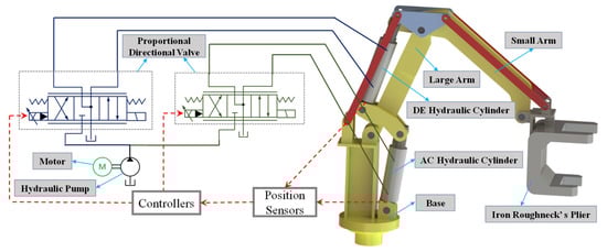
Figure 1.
Principle of the mechanical arm of the iron roughneck system.
2.2. Kinematic Modelling of an MAIR
As the clamp head position of the MAIR is jointly determined by the displacement of the two hydraulic cylinders, modelling the kinematics of the moving arm mechanism to plan the spatial trajectory of the pincer head is necessary. Kinematic modelling includes forward and inverse kinematics. Forward kinematics is used for determining the displacement of the two hydraulic cylinders, which can obtain the position of the workspace of the clamp head. The inverse kinematics of an iron roughneck gives the position of the clamp head in the workspace to obtain the displacement of the two hydraulic cylinders. Figure 2 shows a schematic of an MAIR. The origin of the workspace X-Y was set at point on the iron roughneck’s base. The connection point between the clamp head and big arm was considered as the trajectory planning point. Point J was the center of gravity of the clamp head, and the total gravity of the clamp head was . According to a sketch of the mechanism, the following relationship can be obtained:
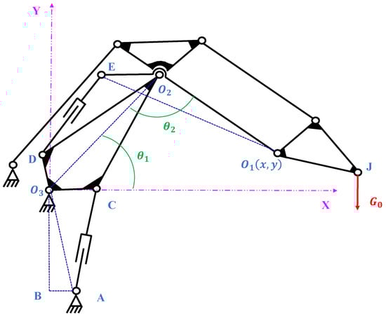
Figure 2.
Sketch of MAIR.
Forward kinematics can be realized using the analytical method, simplifying and for a two-link mechanism, and establishing a coordinate expression of point in the working space as follows:
Equations (1)–(4) are the kinematic positive solution formulae, where the displacements of the two hydraulic cylinders are and , given the length of the two hydraulic cylinders, to obtain the coordinates of point .
The kinematic inverse solution is essential for the working space position control of the iron roughneck. The iron roughneck jaw needs to run according to a specific trajectory, and the length of the hydraulic cylinder and end position are nonlinear; therefore, an inverse solution is needed to obtain the displacement change curve of the hydraulic cylinder, and the displacement signal obtained from the inverse solution is used as the control signal of the hydraulic cylinder.
The inverse kinematic equation is as follows:
2.3. Iron Roughneck’s End Point Trajectory Planning
The role of the MAIR is to smoothly send the pincer head to the target position; the actual work should ensure that the running trajectory of the pincer head is as smooth as possible. According to the operating conditions, the trajectory of the MAIR in the working space is designed as a circular arc, and the highest point of the circle is taken as the target point of the iron roughneck, because the rate of change in the iron roughneck in the Y-direction at this point is zero. This can ensure that the end of the iron roughneck reaches horizontal. The radius of the arc was set according to the starting point to ensure that both the starting and target points were on the same arc. The running trajectory at the end of the iron roughneck is shown in Figure 3.
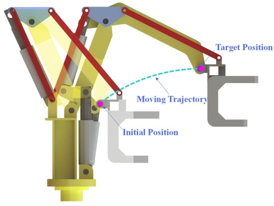
Figure 3.
The end of the MAIR running track.
The coordinates of each interpolated point can be obtained by taking equidistant points on the X-axis corresponding to the trajectory between the initial and end points and calculating the Y value corresponding to each X. The displacement of the two hydraulic cylinders corresponding to each interpolation point was obtained using the kinematic inverse solution, at which point the trajectory-planning problem in the workspace was transformed into the joint space. Using an appropriate heuristic algorithm in the joint space, the system automatically selects the velocities and accelerations of the interpolation points. As shown in Figure 4, the displacements of each interpolation point in the joint space were reasonably selected, and these displacements were represented by small straight-line segments, which are the tangents of the curve at each interpolation point. The interpolation points were assumed to be connected by straight-line segments. If the slope of these lines changed sign at the interpolation point, the velocity was selected as zero. If the slopes of these lines did not change sign, the average of the slopes of the lines on both sides of the interpolation point was selected as the velocity at that point. Based on this method, the system can automatically select the velocity of each interpolation point only according to the specified desired interpolation point. The acceleration was selected based on the velocity that had been generated, and the velocities at the interpolation points were connected by straight-line segments. If the slope of these lines did not change sign, the average of the slopes of the lines on both sides of the interpolation point was selected as the acceleration at that point [32]. During the actual operation of the iron roughneck, ensuring that the velocity and acceleration at the initial and termination points are 0 is necessary.
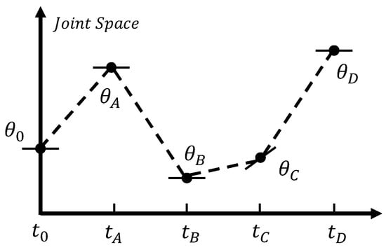
Figure 4.
Interpolation points with desired velocity at points marked with tangent lines.
The velocity and acceleration of the spatial interpolation points of the iron roughneck joint can be obtained using the above algorithm, and the smooth displacement, velocity, and acceleration curves can be obtained by fitting the quintic polynomial. The expressions for the quintic polynomial used for fitting are as follows:
where , , …, are the parameters to be determined, and six constraints are required; that is, information about the displacement, velocity, and acceleration at the initial and termination points. The endpoint conditions for the interpolation are
where , , and are the displacement, velocity, and acceleration at the initial point, respectively. , , and are the displacement, velocity, and acceleration at the termination point, respectively.
If , six coefficients can be obtained:
For the case of n interpolation points, the above formula can be applied to all two adjacent points to obtain the final interpolation curve. Figure 5 shows the joint space curve of displacement, velocity, and acceleration after interpolation for 10 s, and the dot in the figure is the selected six interpolation points. As can be observed, the velocity and acceleration of the joint space trajectory after interpolation were continuous and smooth. The interpolated curve was mapped to the time axis to obtain the hydraulic cylinder displacement control signal, which ensured the smoothness of the motion and helped reduce joint shock.
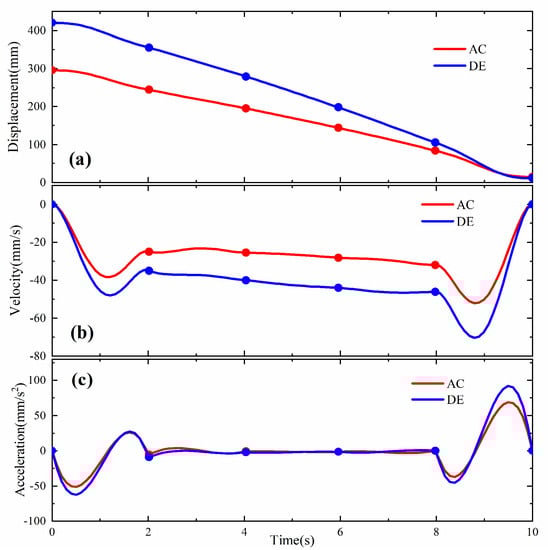
Figure 5.
Trajectory of the joint space of the hydraulic cylinder after interpolation. (a) Displacement curves for trajectory planning; (b) velocity curves for trajectory planning; (c) acceleration curves for trajectory planning.
2.4. Mathematical Modelling of the Hydraulic System of the MAIR
The hydraulic system of an iron roughneck mainly consists of two PVCSE cylinder branches, both of which are position servo systems. The PVCSE hydraulic cylinder position servo system consists of electro-hydraulic servo valves, asymmetric hydraulic cylinders, hydraulic pumps, position sensors, and other components. Establishing a transfer function for the hydraulic servo valve and asymmetric cylinder was key to this study. The two PVCSE cylinder branches were identical and were modelled for only one branch. Figure 6 shows the PVCSE hydraulic cylinder model.
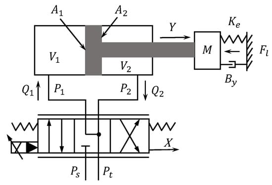
Figure 6.
PVCSE hydraulic cylinder model.
In a symmetric valve-controlled asymmetric cylinder system, due to the hydraulic cylinder area not being equal, the hydraulic cylinder in the left and right direction of the open-loop gain are not equal, resulting in the piston forward and reverse image movement not having the same transfer function, meaning the basic equations of the power mechanism need to be considered separately when writing. The derivation process in both directions is basically the same, and only one direction is considered in this paper. For the derivation process, we referred to [33], and some parameter symbols are defined in Table 1.

Table 1.
Symbols and definitions of each physical quantity of the hydraulic system.
2.4.1. Load Pressure-Flow Characteristics of Servo Valves
As can be observed from Figure 4, each physical quantity was positive in the direction of the arrow, and the flow equation of the servo valve was given by the positive movement of the hydraulic cylinder, Y > 0.
The flow rate through the two throttling windows of the servo valve was not equal to the load flow rate and was defined as
where .
Given that the piston moves slightly around the steady-state operating point frequently during the normal operation of the hydraulic system, and considering the effect of the flow pressure coefficient, while equating the flow gain and the flow pressure coefficient as constants, the Taylor series expansion near the operating point and flow equation was linearized as
where ;, with a zero position flow pressure coefficient of 0; .
2.4.2. Flow Continuity Equation for Valve-Controlled Hydraulic Cylinders
2.4.3. Force Balance Equations for Asymmetric Hydraulic Cylinders and Loads
Simplifying Equation (15) yields:
2.4.4. Mathematical Model of the Displacement of a PVCSE Hydraulic Cylinder
Equations (13), (14) and (16) are Laplace transforms, and the mathematical model of the displacement of a PVCSE hydraulic cylinder is obtained by combining
2.4.5. Transfer Functions for Position Closed-Loop Control Systems
In a position control system where the cylinder displacement is the output quantity, the elastic load can be ignored; that is, . In addition, the total coefficient is negligible and the viscous friction coefficient is also negligible. Hence, , which can be ignored. The entire transfer function can be reduced to
where : hydraulic inherent frequency, ; : hydraulic damping ratio, and .
The linear joint of the iron roughneck is formed by two members moving relatively ton one another using articulation, and the earrings of the head and tail of the linear asymmetric hydraulic cylinder are articulated on the two members of the joint. The required movement angle is achieved by the expansion and contraction of the PVCSE hydraulic cylinder, and then the position information feedback is completed by the built-in sensor of the hydraulic cylinder. In most servo systems, the dynamic response of the servo valve is typically higher than that of the power element. To simplify the analysis and design of the system dynamic characteristics, the transfer function of the servo valve displacement to the input current can be approximated using a proportional link. The servo amplifier is a voltage-to-current converter with high output impedance. The frequency band is significantly higher than the inherent hydraulic frequency, which can also be simplified as a proportional link. The transfer function of the displacement transducer can be considered a proportional link. The servo valve, amplifier, and displacement transmitter gains were (), (), and (), respectively.
Equation (18) shows that the output displacement of the iron roughneck-driving hydraulic cylinder is affected by the servo-valve opening and external load. When the external load , only changing the external load to constitute different servo systems and adapting to different linear joint requirements, such as the up and down swing of the iron roughneck’s big arm and the back-and-forth swing of the small arm, are necessary, all of which can be dynamically analyzed on this basis. For , the servo-valve spool opening directly determines the output displacement of the hydraulic cylinder. The hydraulic valve-controlled system is a third-order system consisting of an integral link and a second-order oscillating link, and there is a case where the pole = 0. In this case, the pole is not all in the negative axis, which may be an unstable system. According to the stability criterion of the hydraulic position control system in reference [33], from , it can be seen that the stability condition is satisfied according to the characteristic parameters of the system calculated. Therefore, this hydraulic position control system is stable. A square diagram of the closed-loop system is shown in Figure 7.
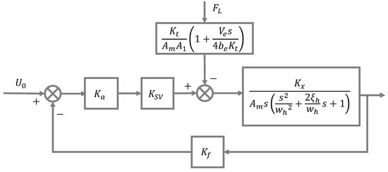
Figure 7.
Control block diagram of position closed-loop system.
2.5. Controller Design
The control principle of the MAIR is shown in Figure 8. The trajectory planning is divided into workspace trajectory planning and joint space trajectory planning. The generation of the position signal of the hydraulic cylinder takes place during the joint space trajectory planning. The MAIR provides an equivalent the displacement signal to the hydraulic cylinder for control, the servo valve model is established to simulate the hydraulic system of iron roughnecks, and the control is actually the proportional reversing valve in the hydraulic system, so it is necessary to establish a servo valve model to study the control of electro-hydraulic position system. The output of the controller is transmitted to the proportional reversing valve, which controls the valve opening of the proportional reversing valve through a given electrical signal from the controller, and the flow rate is then controlled to realize the position control of the hydraulic cylinder. The position signal of the target hydraulic cylinder is fed back to the controller through a position sensor.
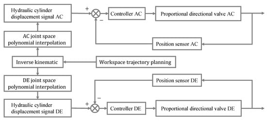
Figure 8.
Hydraulic cylinder control principle.
2.5.1. ADRC
The ADRC consists of a TD, ESO, and NLSEF [34]. The TD smoothly approximates the generalized derivative of the input signal. The ESO estimates the output and total real-time perturbation. The NLSEF uses the total perturbation observed by the ESO to generate control variables, thus ensuring system stability. The principle of the ADRC is shown in Figure 9.
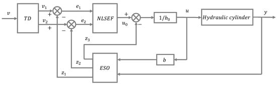
Figure 9.
ADRC principle.
2.5.2. TF-ADRC
The principle of a TF-ADRC is based on an ADRC and introduces two tracking differentiators to realize the tracking of discontinuous signals, extract the error, error change rate, and error change acceleration rate, and uses linear error feedback to improve the response speed. By combining fuzzy control and an ADRC controller, the output signal of the controller is dynamically compensated for by the displacement deviation, displacement deviation change rate, and displacement deviation change acceleration rate of the hydraulic cylinder. The system parameters have the characteristics of a ‘large error, large compensation’ and ‘small error, small compensation’. The entire control system has higher robustness and faster response speed. Figure 10 shows the principle of the TF-ADRC. The design of the controller includes the fuzzy link and the ADRC design of the three-dimensional input.
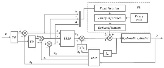
Figure 10.
Three-dimensional fuzzy ADRC principle.
2.6. Tracking Differentiator
To avoid the noise amplification of traditional differential links, the TD achieves a smooth approximation of differential inputs, which handles noise better than traditional differential methods. The use of the double TD can realize a smooth transition of displacement, velocity, and acceleration. Considering the displacement of the hydraulic cylinder as an example, the expression of the nonlinear second-order tracking differentiator was designed as follows:
where is the fastest control synthesis function of the system used to build the discrete tracking differentiator. Specifically, it is expressed as
where and are the input and output of the tracking differentiator, respectively, is the differentiated output of , is the adjustable tracking speed, and and are the analog intervals of the TD and functions, respectively. The larger the , the larger the oscillation. When , the high-frequency oscillation of can be eliminated; when , the noise of can be eliminated.
2.7. Three-Dimensional Fuzzy Module
Recently, fuzzy control theory has attracted considerable attention in the control community and has been widely used in many fields. However, current fuzzy control research mainly focuses on the application of two-input fuzzy control methods; multiple-input cases have not been sufficiently investigated, especially the theoretical analysis and exploration of fuzzy controllers, which are found to be superior, more robust, faster, more flexible, and more insensitive to parameter changes than traditional two-input fuzzy controllers [35]. The principle of the three-input fuzzy module is illustrated in Figure 11.
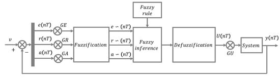
Figure 11.
Fuzzy controller with three-dimensional input.
The fuzzy controller adds an error-variation acceleration rate as an input with respect to a typical two-input fuzzy controller. The sampling period was assumed to be small and all measurements were assumed to be free of noise. The labels in Figure 11 are as follows:
In Equation (21), is a positive integer; is the set target value, which can be the displacement; is the sampling period; and , , , , and are the error, error rate of change, error rate of change acceleration, system output, and fuzzy controller output at sampling moment , respectively. , , and denote the sampling values at the moment. GE, GR, GA, and GU are the error gain, error change rate gain, error change acceleration rate gain, and output gain, respectively. denotes fuzzification, denotes the controller output increment, and the fuzzy controller sets the exact output increment at the moment. , , and are the fuzzy set pairs of , , and responses, respectively.
2.8. Design of Fuzzification and Fuzzy Control Rules
Fuzzification needs to be realized by the affiliation function, and here, a simple triangular affiliation function was used to define the fuzzy subsets of the input quantities as small (S), medium (M), and large (L), and the fuzzy subsets of the output quantities as very small (VS), small (S), medium (M), large (L), and very large (VL). The input and output incremental fuzzification algorithms are shown in Figure 12.
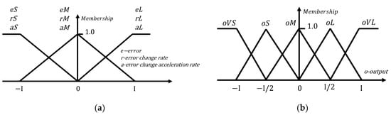
Figure 12.
Fuzzy affiliation functions. (a) Input affiliation function; (b) output affiliation function.
The hydraulic cylinder displacement deviation , displacement deviation change rate , and displacement deviation change acceleration rate were used as the fuzzy controller inputs, and the compensation amount fuzzy of the ADRC control quantity was used as the fuzzy controller output. The linguistic variables of the input and output were as follows:
Fuzzy rules are defined according to the defined subordinate functions of the input and output, and fuzzy rules are usually created with expert experience, which reflects the output regulation law of fuzzy control. The controller of this three-dimensional input needed to design 27 fuzzy rules, which are summarized in Table 2. According to the affiliation function of the input and output, the control rules are designed (Table 2), where the first and second rows of the horizontal coordinate are the hydraulic cylinder displacement deviation and hydraulic cylinder displacement deviation change rate , respectively, and the vertical coordinate is the hydraulic cylinder deviation change acceleration rate . According to Table 2, when S, S, and S, the corresponding output language variable VS; when M, M, and L, the corresponding output language variable L, and so on.
Table 2.
Fuzzy rule table for three-dimensional input.
The Mamdani method [36] was used for fuzzy inference, and the Mamdani inference method used the Cartesian product of A and B to represent the fuzzy implication relation A → B. The Fuzzy module in MATLAB is based on the Mamdani inference method. For the case of linguistic rules containing multiple inputs, suppose the fuzzy relationship between the input linguistic variables and output variable is . When the fuzzy values of the output variables are , respectively, the corresponding takes the value , which can be obtained by fuzzy inference as follows:
The output quantity of the fuzzy controller was a fuzzy set, and the exact quantity was adjudicated using the inverse fuzzification method. Among many inverse fuzzification methods, the center-of-gravity method was selected in this study. The center-of-gravity method takes the center of gravity of the area enclosed by the fuzzy affiliation function curve and horizontal coordinate axis as the representative point. In most cases, the numerical integration method is used for calculation.
where is the clear value of the fuzzy controller output, represents the ith theoretical domain after discretization, represents the corresponding affiliation at , and is the output scaling factor.
2.9. Extended State Observer
The ESO is the core of the ADRC, and its role was to estimate the total real-time disturbance of the system and translate it into new state variables to compensate for the controller’s output. Then, all the state variables were observed using the inputs and outputs of the system.
where , , , and are estimates of the target signal and , respectively. is the total disturbance estimate for the system. , and , are the four constants in the ESO, which were determined by Equation (26).
2.10. Linear State Error Feedback Law
The error during the transition can be tracked based on TD and ESO. A linear or non-linear approach was used to construct the feedback control law such that the steady-state error gradually reduced and the output response accelerated. In this study, a linear construction was used, and the controller calculated its output based on a linear combination of the difference between the estimated and true state variables, as shown in Equation (27).
where and , , and are scale factors.
2.11. Disturbance Compensation Process
Perturbation compensation in Equation (28) depends on the real-time estimated total perturbation in the ESO.
The output consists of three components: , the compensated disturbance component; , the integrator level component controlled by nonlinear feedback; and , the compensation of the fuzzy module for the output.
3. Results and Discussion
The AMESim-Simulink simulation model was established using the equations of the hydraulic system as previously described. The reliability of the established simulation model of the hydraulic system of the MAIR was verified through experiments. Figure 13 shows the experimental system.
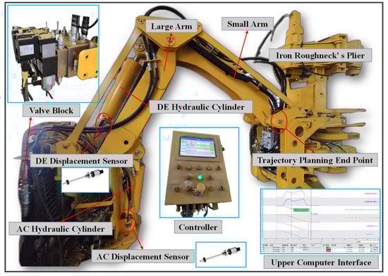
Figure 13.
Experimental system. Upper Computer Interface: First line (轨迹算法测试输出_ac). Second line (轨迹算法测试输出_de): It is the output of the proportional directional valve obtained according to the algorithm of trajectory planning, which is an electrical signal representing the valve opening of the proportional valve.( ac and de correspond to the proportional valves that control the AC and DE hydraulic cylinders). 插补算法: Planned hydraulic cylinder operation trajectory. 信号基…: Output signal serial number of controller. 名称: Output signal name of controller. 数据类型: Data type of the signal. 显示格式: Display Format. 浮点: Floating point. 地址: Address. 公式: Formula. 颜色: Color. 信号组: Signal group. Y轴最小: Y-axis minimum. Y轴最大: Y-axis maximum.
Figure 14a,b shows the tracking of the AC and DE hydraulic cylinders for the planned hydraulic cylinder displacement curve, respectively. As can be observed in the experiment, the tracking of the physical MAIR with the AMESim simulation model for the planned trajectory was approximately the same when the PID control scheme was used. The maximum deviation allowed for the displacement tracking trajectory of IRMA hydraulic cylinders is ±20 mm. The trajectory tracking errors of the experimental and simulation models of the AC and DE hydraulic cylinders in Figure 14 were both within 20 mm, which meet the engineering requirements.
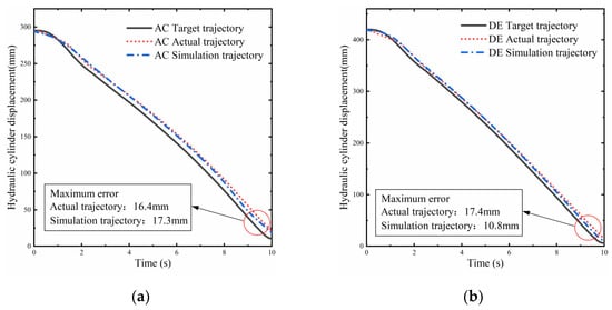
Figure 14.
Tracking of the experimental equipment and simulation model for the planned trajectory. (a) AC hydraulic cylinder trajectory tracking; (b) DE hydraulic cylinder trajectory tracking.
The engineering requirement for velocity trajectories is to be as smooth as possible. Trajectory planning allows for better velocity tracking of the position control system. Figure 15 shows the tracking of speed between the experiment and simulation. It was seen that the overall speed change in the simulation was smooth, while the speed of the experimental result exhibited a jitter. This is due to the influence of friction and hydraulic oil temperature change in the actual operation of the MAIR, which was not considered in the simulation model. This causes the speed of the hydraulic cylinder to be tracked imperfectly on the planned trajectory in the simulation and experiment. Overall, the displacement and velocity tracking errors were within an acceptable range, and the experiment verified the reliability of the simulation model.
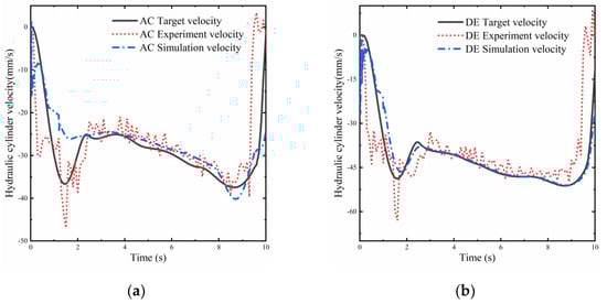
Figure 15.
Velocity tracking of the experimental equipment and simulation model for the planned trajectory. (a) AC hydraulic cylinder velocity tracking; (b) DE hydraulic cylinder velocity tracking.
To compare and verify the performance of several controllers, controller simulation models for a PID controller, fuzzy PID controller, ADRC, and TF-ADRC were built. The fuzzy modules in the fuzzy PID controller and TF-ADRC were built using the fuzzy toolbox in MATLAB and Figure 16 shows the simulation model of the controllers.
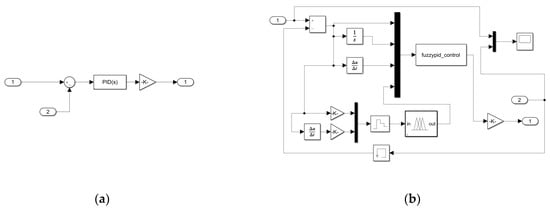
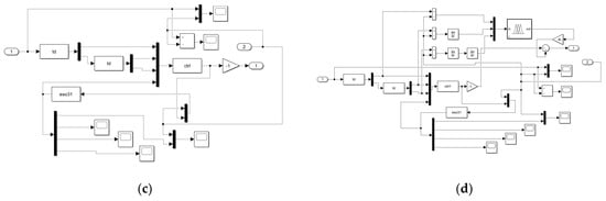
Figure 16.
The simulation model of the controllers. (a) PID controller; (b) fuzzy PID controller; (c) ADRC; (d)TF-ADRC.
Several working conditions were separately designed for testing. The barrel and rod diameters of the AC and DE hydraulic cylinders were the same: 150 and 75 mm, respectively. The maximum strokes of the AC and DE cylinders were 300 and 420 mm, respectively; the other parameters of the two hydraulic cylinder branches were the same, and a marker was used here to indicate them. The parameters of the PID controller were rectified using the genetic algorithm module included with AMESim, and relatively optimal PID parameters were obtained. The parameters of the fuzzy PID controller were adjusted based on the rectified PID parameters. The adjusted and fuzzy PID controllers can achieve optimal control performance, which provides a basis for the performance comparison of different controllers. The parameters of the hydraulic system refer to the parameters of iron roughnecks in engineering projects, as well as the parameters in reference [33], some of which are commonly used in the engineering experience, and some of the parameters of the controller are those tested through simulation experiments with relatively good results. Some of the parameters of the hydraulic system and controller are listed in Table 3.
Table 3.
Some parameters of the hydraulic system and controller.
As shown in Figure 17a,b, the response of two hydraulic cylinders with different control methods to the step square wave signal was verified by applying a load of 30,000 N for 0.5 s in opposite directions at 7 s and 15 s. Whether the hydraulic cylinder extends or retracts, the system generates a certain disturbance, as shown by Equation (18); the system model, system pressure, flow rate, and displacement of the hydraulic cylinder change with changes in the external load FL. As can be observed, the response times of the ADRC and TF-ADRC were faster, both reaching a steady state within 2 s, while the PID and fuzzy PID controllers required a longer time to reach the target point, reaching a steady state at approximately 3 s. At the 7 and 15 s positions, the ADRC and TF-ADRC exhibited less error under load disturbance because the self-anti-disturbance controller generates a faster and higher amplitude control signal when the step load disturbs the system output, making the system respond faster and reducing the effect of the disturbance on the system. Figure 17c,d shows the step response under a sinusoidal load . The steady-state error of the system using self-rejecting control was less than that of the system using a PID controller, indicating that the system with the ADRC is more robust and can adapt well to the effects of system model changes and load perturbations because the ESO module of the ADRC predicts the output and total real-time perturbations of the system and the LSEF module generates corresponding control quantities based on the perturbations. Figure 17e,f shows the tracking of the two hydraulic cylinders for a sinusoidal signal at a constant load of 10,000 N. The results show that the system with the ADRC and TF-ADRC exhibited a better input tracking performance, and the system with PID and fuzzy PID controllers exhibited more hysteresis. The tracking effects of the PID and fuzzy PID controllers are no longer satisfactory for complex signals when the hydraulic cylinder has a large load. To further investigate the comprehensive performance of the ADRC and TF-ADRC, random loads of −30,000–30,000 N were set in the AC and DE cylinders, as shown in Figure 17g,h, and sinusoidal signals were tracked. Both the PID and fuzzy PID controllers have unsatisfactory tracking effects under variable load conditions, which indicate that the PID control strategy finds it difficult to adapt to to complex conditions, whereas the ADRC-based control strategy can generate stronger control signals to compensate for the error caused by high-load conditions and has better overall anti-interference capability.
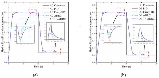
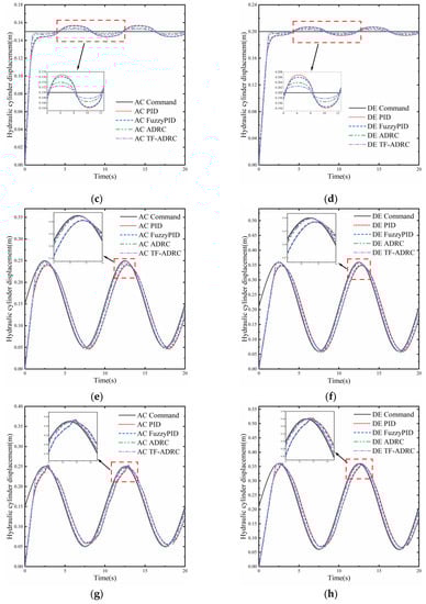
Figure 17.
Displacement tracking of two hydraulic cylinders for different working conditions. (a) Response of AC hydraulic cylinder to square wave signal under a sudden change in load; (b) response of DE hydraulic cylinder to square wave signal under a sudden change in load; (c) response of AC hydraulic cylinder to step signal under sinusoidal load; (d) response of DE hydraulic cylinder to step signal under sinusoidal load; (e) response of AC hydraulic cylinder to sinusoidal signal under constant load; (f) response of DE hydraulic cylinder to sinusoidal signal under constant load; (g) response of AC cylinder to sinusoidal signal under random load; (h) response of DE cylinder to sinusoidal signal under random load.
Table 4 shows the response data of the two hydraulic cylinders to the square wave signal. Analysis shows that the performance of the TF-ADRC was improved compared with the traditional PID controller and ADRC, and the control accuracy was higher than the latter. Taking the AC hydraulic cylinder as an example, the response time of extension and retraction of the TF-ADRC was 1.40 s and 1.55 s, the maximum steady-state error was 3.48 mm and −4.05 mm, and the average steady-state error was 0.31 mm and −0.42 mm, respectively. When using the ADRC controller, the response time was 1.46 s and 1.67 s, the maximum steady-state error was 5.78 mm and −6.78 mm, and the average steady-state error was 0.59 mm and −0.71 mm. When using the PID controller, the response time was 1.73 s and 2.51 s, the maximum steady-state error was 8.15 mm and −10.30 mm, and the average steady-state error was 0.92 mm and −1.33 mm. When using the fuzzy PID controller, the response time was 1.68 s and 2.54 s, the maximum steady-state error was 7.32 mm and −9.47 mm, and the average steady-state error was 0.85 mm and −1.21 mm, respectively. Compared with the ADRC, the response time was reduced by 4.11% and 7.19%, the maximum steady-state error was reduced by 39.8% and 40.3%, and the average steady-state error was reduced by 47.5% and 40.8%, respectively. Compared with the PID controller, the response times of the extension and retraction were reduced by 19.1% and 38.2%, respectively; the maximum steady-state errors were reduced by 57.3% and 60.7%, respectively; the average steady-state errors were reduced by 66.3% and 68.4%, respectively. Compared with the fuzzy PID controller, the response times of the extension and the retraction controller were reduced by 16.7% and 39.0%, respectively; the maximum steady-state errors were reduced by 52.0% and 57.2%, respectively; the average steady-state error were reduced by 63.5% and 65.3%, respectively.
Table 4.
Comparison of controller simulation data.
Figure 18 shows the performance of the controller for a step signal under sinusoidal load. The TF-ADRC has a faster response, smaller maximum steady-state error, and smaller average steady-state error than other controllers. This indicates that the TF-ADRC has good robustness against load variations.
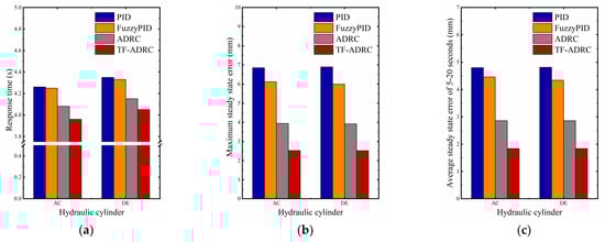
Figure 18.
Controller dynamic performance comparison. (a) Response time of controller; (b) maximum steady-state error of the controller; (c) average steady-state error of the controller at 5–20 s.
Figure 19 shows the estimated states and the total disturbances. The observed value jittered more at the beginning because the hydraulic cylinder speed and acceleration changed more drastically, and the ESO was highly sensitive to the signal and disturbance of the three-dimensional input, but the overall observation accuracy was acceptable after 3 s. The TF-ADRC had more ESO observation error than the ADRC because of the compensation effect of the FL module on the LSEF output, so that the TF-ADRC achieved a faster response and higher driving accuracy. The perturbation and uncertain parameters estimated by ESO greatly enhance the robustness of the system.
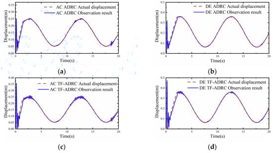
Figure 19.
ESO observation results under the random load. (a) ESO observation of the ADRC controller for AC hydraulic cylinders; (b) ESO observation of the ADRC controller for DE hydraulic cylinders; (c) ESO observation of the TF-ADRC controller for AC hydraulic cylinders; (d) ESO observation of the TF-ADRC controller for DE hydraulic cylinders.
To verify the application effect of the TF-ADRC on the MAIR, the dynamics model of the MAIR was established based on RECURDYN, and a vertical downward constant load was applied to the clamp head to simulate the real force situation of the iron roughneck during operation, as shown in Figure 20.
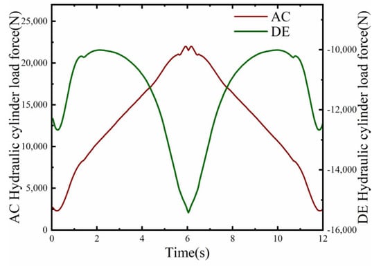
Figure 20.
Joint simulation of load forces.
The trajectories of the forward and backward iron roughnecks were circular arcs, and the displacement control signals of the two hydraulic cylinders were generated using five-fold polynomial interpolation. Figure 21 compares the tracking effect of the four controllers for the planned trajectory, and as can be seen, the ADRC and TF-ADRC exhibited higher position control accuracies than the PID and fuzzy PID controllers.
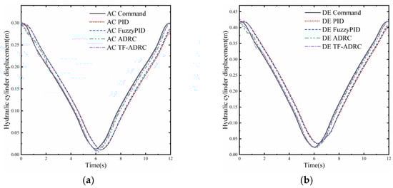
Figure 21.
Tracking of the two hydraulic cylinders for the planned trajectory. (a) Tracking of planned trajectories by AC hydraulic cylinder; (b) tracking of planned trajectories by DE hydraulic cylinder.
However, the ADRC-based controller showed a large jump in the initial control, and the smoothness for speed was not comparable with the PID controller for speed tracking, as shown in Figure 22.
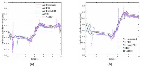
Figure 22.
Velocity tracking of two hydraulic cylinders. (a) Velocity tracking of AC hydraulic cylinders for planned trajectory; (b) velocity tracking of DE hydraulic cylinders for planned trajectory.
Although the ADRC-based controller has higher position control accuracy and stronger robustness in an electro-hydraulic position control system, it is undeniable that its velocity tracking characteristics do not work well. Initially, a large jump was observed in the linear expansion state observer, resulting in a more drastic change in the control signal at the beginning, and the speed change curve was not smooth throughout the process because the ADRC controller is very sensitive to the change in error and outputs a drastically changing control signal, which is not allowed in engineering. To solve this problem, consider constraining the controller output with a limiter in the initial stage, which can effectively improve the jumping problem in the initial stage of the ADRC controller, and add a filter throughout the operation to smooth the ADRC output, although this may also decrease the position control accuracy. In summary, PID and fuzzy PID control cannot adapt well to system model changes and load disturbances, whereas the ADRC and TF-ADRC improved the position control accuracy of the system when the control object parameters were changed and external load disturbance occurred. The designed TF-ADRC control strategy exhibited better robustness and anti-interference capability than the ADRC, which provides a reference for practical engineering applications.
4. Conclusions
In this study, the trajectory tracking control algorithm of an MAIR was investigated. The main innovations of this work are as follows:
(1) The mathematical model of the MAIR and hydraulic system was established, the trajectories of the two hydraulic cylinders were planned using the quintic polynomial interpolation algorithm. The planned trajectories of the hydraulic cylinders have the characteristics of smooth velocity and acceleration. The smooth connection of the velocity of the hydraulic cylinders at the interpolation point was realized.
(2) A control strategy of a TF-ADRC for the MAIR was proposed. The TF-ADRC was designed to realize the smoothing of the input signal by the double TD module. The fuzzy module of three-dimensional input was designed to compensate for the output of the ADRC controller according to the tracking deviation, deviation change rate, and deviation change acceleration rate.
(3) A joint AMESim-Simulink simulation model was built, and the reliability of the simulation model and trajectory planning method was verified through experiments. The feasibility of applying a fuzzy PID controller, ADRC, and TF-ADRC to the MAIR was verified through the simulation model, which provides a reference for the application of the new control strategy in engineering.
(4) Different control strategies were compared using the simulation model. TF-ADRC was found to exhibit a higher trajectory tracking accuracy, response speed, and stability than the PID controller, fuzzy PID controller, and ADRC. In the case of external disturbances, the controller exhibited stronger robustness.
The research presented in this paper provides the basis for the trajectory tracking control of MAIRs with large load variations. However, the modelling of the hydraulic system in this study did not consider oil temperature, friction, and other factors, and simplifies the pressure station as an ideal constant pressure source. In actual engineering applications, the oil temperature in an electro-hydraulic servo system has a non-negligible influence on control accuracy. The subsequent consideration is to establish a more accurate hydraulic system model to further verify the reliability of the TF-ADRC and to further study the speed smoothing control of the TF-ADRC. In addition, experiments will be added in the future to verify the effect of the TF-ADRC on iron roughnecks. It can be probably be practically applied to oil drilling equipment to improve equipment operation accuracy and efficiency.
Author Contributions
K.Z. and Y.L. contributed to the conceptualization and performed the experiments; F.Y. designed the structure and the hydraulic circuit; K.Z. designed the controller and wrote the paper; H.J. analyzed the data; G.X. reviewed and edited the paper; Y.L. and G.X. contributed to the funding acquisition, supervision, and project administration. All authors have read and agreed to the published version of the manuscript.
Funding
The research was supported by the National Natural Science Foundation of China [no. 52001186], the Natural Science Foundation of Shandong Province [no. ZR2020QE292], the Open Fund of State Key Laboratory of Mechanical Transmission [no. SKLMT-KFKT-202214], the Key Research and Development Plan of Shandong Province—Major Science and Technology Innovation Project [no. 2022CXGC010608], for which the authors are grateful.
Data Availability Statement
Data are available on request due to restrictions e.g., privacy or ethical. The data presented in this study are available on request from the corresponding author. The data are not publicly available due to the presence of some confidential information.
Acknowledgments
We gratefully acknowledge the experiment provided by Beijing Jiejiexi Petroleum Equipment Co., Ltd.
Conflicts of Interest
There are no conflict of interest regarding the research for this thesis.
References
- Zhan, Z.; Sha, Y.; Wang, Q.; Piao, C.; Liu, X. Optimization of the hinge point position of the articulated boom for SP-I-04-Type iron roughneck. J. Harbin Eng. Univ. 2015, 36, 205–208. [Google Scholar]
- Chao, Q.; Zhang, J.H.; Xu, B.; Huang, H.P.; Pan, M. A Review of High-Speed Electro-Hydrostatic Actuator Pumps in Aerospace Applications: Challenges and Solutions. J. Mech. Des. 2019, 141, 13. [Google Scholar] [CrossRef]
- Kim, J.H.; Hong, Y.S. Improvement of Backdrivability of a Force-Controlled EHA by Introducing Bypass Flow Control. Int. J. Precis. Eng. Manuf. 2020, 21, 819–830. [Google Scholar] [CrossRef]
- Fu, Y.L.; Han, X.; Sepehri, N.; Zhou, G.Z.; Fu, J.; Yu, L.M.; Yang, R.R. Design and performance analysis of position-based impedance control for an electrohydrostatic actuation system. Chin. J. Aeronaut. 2018, 31, 584–596. [Google Scholar] [CrossRef]
- Du, C.; Plummer, A.R.; Johnston, D.N. Performance analysis of a new energy-efficient variable supply pressure electro-hydraulic motion control method. Control Eng. Pract. 2017, 60, 87–98. [Google Scholar] [CrossRef]
- Pu, Y.S.; Shi, Y.Y.; Lin, X.J.; Zhang, W.B.; Zhao, P. Joint Motion Planning of Industrial Robot Based on Modified Cubic Hermite Interpolation with Velocity Constraint. Appl. Sci. 2021, 11, 8879. [Google Scholar] [CrossRef]
- Song, Q.S.; Li, S.B.; Bai, Q.; Yang, J.; Zhang, A.S.; Zhang, X.X.; Zhe, L.X. Trajectory Planning of Robot Manipulator Based on RBF Neural Network. Entropy 2021, 23, 1207. [Google Scholar] [CrossRef]
- Yang, Y.L.; Wei, Y.D.; Lou, J.Q.; Fu, L.; Zhao, X.W. Nonlinear dynamic analysis and optimal trajectory planning of a high-speed macro-micro manipulator. J. Sound Vibr. 2017, 405, 112–132. [Google Scholar] [CrossRef]
- Wang, D.; Dong, Y.X.; Lian, J.; Gu, D.B. Adaptive end-effector pose control for tomato harvesting robots. J. Field Robot. 2023, 40, 535–551. [Google Scholar] [CrossRef]
- Aboud, W.S.; Haris, S.M.; Yaacob, Y. Advances in the control of mechatronic suspension systems. J. Zhejiang Univ. Sci. C 2014, 15, 848–860. [Google Scholar] [CrossRef]
- Sun, X.X.; Lu, Z.X.; Song, Y.; Cheng, Z.; Jiang, C.X.; Qian, J.; Lu, Y. Development Status and Research Progress of a Tractor Electro-Hydraulic Hitch System. Agric. 2022, 12, 1547. [Google Scholar] [CrossRef]
- Liu, G.P.; Daley, S. Optimal-tuning nonlinear PID control of hydraulic systems. Control Eng. Pract. 2000, 8, 1045–1053. [Google Scholar] [CrossRef]
- Fan, Y.Q.; Shao, J.P.; Sun, G.T. Optimized PID Controller Based on Beetle Antennae Search Algorithm for Electro-Hydraulic Position Servo Control System. Sensors 2019, 19, 2727. [Google Scholar] [CrossRef] [PubMed]
- Guo, Y.Q.; Zha, X.M.; Shen, Y.Y.; Wang, Y.N.; Chen, G. Research on PID Position Control of a Hydraulic Servo System Based on Kalman Genetic Optimization. Actuators 2022, 11, 162. [Google Scholar] [CrossRef]
- Ye, Y.; Yin, C.B.; Gong, Y.; Zhou, J.J. Position control of nonlinear hydraulic system using an improved PSO based PID controller. Mech. Syst. Signal Process. 2017, 83, 241–259. [Google Scholar] [CrossRef]
- Cetin, S.; Akkaya, A.V. Simulation and hybrid fuzzy-PID control for positioning of a hydraulic system. Nonlinear Dyn. 2010, 61, 465–476. [Google Scholar] [CrossRef]
- Ghosh, B.B.; Sarkar, B.K.; Saha, R. Realtime performance analysis of different combinations of fuzzy-PID and bias controllers for a two degree of freedom electrohydraulic parallel manipulator. Robot. Comput.-Integr. Manuf. 2015, 34, 62–69. [Google Scholar] [CrossRef]
- Truong, H.V.A.; Tran, D.T.; To, X.D.; Ahn, K.K.; Jin, M. Adaptive Fuzzy Backstepping Sliding Mode Control for a 3-DOF Hydraulic Manipulator with Nonlinear Disturbance Observer for Large Payload Variation. Appl. Sci. 2019, 9, 3290. [Google Scholar] [CrossRef]
- Zhu, Z.F.; Liu, Y.J.; He, Y.L.; Wu, W.H.; Wang, H.Z.; Huang, C.; Ye, B.L. Fuzzy PID Control of the Three-Degree-of-Freedom Parallel Mechanism Based on Genetic Algorithm. Appl. Sci. 2022, 12, 11128. [Google Scholar] [CrossRef]
- Truong, D.Q.; Ahn, K.K. Force control for press machines using an online smart tuning fuzzy PID based on a robust extended Kalman filter. Expert Syst. Appl. 2011, 38, 5879–5894. [Google Scholar] [CrossRef]
- Han, J. From PID technology to “Active Disturbance Rejection Control” technology. Control Eng. China 2002, 56, 900–906. [Google Scholar]
- Wu, Y.; Zheng, Q. ADRC or adaptive controller—A simulation study on artificial blood pump. Comput. Biol. Med. 2015, 66, 135–143. [Google Scholar] [CrossRef] [PubMed]
- Castaneda, L.A.; Luviano-Juarez, A.; Ochoa-Ortega, G.; Chairez, I. Tracking control of uncertain time delay systems: An ADRC approach. Control Eng. Pract. 2018, 78, 97–104. [Google Scholar] [CrossRef]
- Xue, W.C.; Bai, W.Y.; Yang, S.; Song, K.; Huang, Y.; Xie, H. ADRC With Adaptive Extended State Observer and its Application to Air-Fuel Ratio Control in Gasoline Engines. Ieee Trans. Ind. Electron. 2015, 62, 5847–5857. [Google Scholar] [CrossRef]
- Liu, C.Q.; Luo, G.Z.; Chen, Z.; Tu, W.C.; Qiu, C. A linear ADRC-based robust high-dynamic double-loop servo system for aircraft electro-mechanical actuators. Chin. J. Aeronaut. 2019, 32, 2174–2187. [Google Scholar] [CrossRef]
- Liu, J.J.; Sun, M.W.; Chen, Z.Q.; Sun, Q.L. High AOA decoupling control for aircraft based on ADRC. J. Syst. Eng. Electron. 2020, 31, 393–402. [Google Scholar] [CrossRef]
- Khaled, T.A.; Akhrif, O.; Bonev, I.A. Dynamic Path Correction of an Industrial Robot Using a Distance Sensor and an ADRC Controller. IEEE-ASME Trans. Mechatron. 2021, 26, 1646–1656. [Google Scholar] [CrossRef]
- Zhou, W.; Guo, S.X.; Guo, J.; Meng, F.X.; Chen, Z.Y. ADRC-Based Control Method for the Vascular Intervention Master-Slave Surgical Robotic System. Micromachines 2021, 12, 1439. [Google Scholar] [CrossRef]
- Kang, C.H.; Wang, S.Q.; Ren, W.J.; Lu, Y.; Wang, B.Y. Optimization Design and Application of Active Disturbance Rejection Controller Based on Intelligent Algorithm. Ieee Access 2019, 7, 59862–59870. [Google Scholar] [CrossRef]
- Xu, X.; Wu, Y.; Ni, Y. Adaptive fuzzy auto disturbance rejection control of variable load quadrotor UAV. Transducer Microsyst. Technol. 2022, 41, 101. [Google Scholar]
- Wang, B.; Ji, H.Y.; Chang, R. Position Control with ADRC for a Hydrostatic Double-Cylinder Actuator. Actuators 2020, 9, 112. [Google Scholar] [CrossRef]
- Craig, J.J. Introduction to Robotics Mechanics and Control, 4th ed.; China Machine Press: Beijing, China, 2018; pp. 144–161. [Google Scholar]
- Wu, Z. Hydraulic Control Systems, 1st ed.; Higher Education Press: Beijing, China, 2008; pp. 67–81. [Google Scholar]
- Han, J. Active Disturbance Rejection Control Technique, 1st ed.; National Defense Industry Press: Beijing, China, 2008; pp. 243–280. [Google Scholar]
- Bharathi, Y.H.; Rekha, B.R.; Bhaskar, P.; Parvathi, C.S.; Kulkarni, A.B. Multi-input fuzzy logic controller for brushless de motor drives. Def. Sci. J. 2008, 58, 147–158. [Google Scholar] [CrossRef]
- Fan, L. Some methods of reasoning for fuzzy conditional propositions—Discussion. Fuzzy Sets Syst. 1997, 86, 391–392. [Google Scholar] [CrossRef]
Disclaimer/Publisher’s Note: The statements, opinions and data contained in all publications are solely those of the individual author(s) and contributor(s) and not of MDPI and/or the editor(s). MDPI and/or the editor(s) disclaim responsibility for any injury to people or property resulting from any ideas, methods, instructions or products referred to in the content. |
© 2023 by the authors. Licensee MDPI, Basel, Switzerland. This article is an open access article distributed under the terms and conditions of the Creative Commons Attribution (CC BY) license (https://creativecommons.org/licenses/by/4.0/).