A New Method of Tractor Engine State Identification Based on Vibration Characteristics

Abstract

Based on signal decomposition, a tractor engine state recognition method is proposed to explore the degree of information recognition of vibration signals at measurement points at different distances from the engine and the degree of correlation in different directions. The accuracy of engine operating state information recognition was obtained by analyzing the vibration signals of the tractor at different measurement points. The main contents are as follows: Based on variational mode decomposition (VMD), the modal component, which includes the state information, was obtained by measuring the vibration signal of the tractor at each measurement point under different driving conditions, and the exogenous excitation of the tractor under different road conditions was simulated by changing the tire pressure. Then, the state characteristics of the modal component were quantified based on permutation entropy (PE), and the correlation coefficient was used as the evaluation index to select the entropy of the optimal modal component as the feature vector. Finally, a support vector machine and random forest classification models were trained with 4800 feature vectors under 25 working conditions, and the remaining 900 feature vectors were used to verify the classification results. Compared with the results of empirical mode decomposition (EMD), the superiority of this method was proved. A comparative study with backpropagation demonstrated the superiority of the support vector machine and random forest identification method using a small sample size. The results indicate the following: (1) the accuracy of engine condition recognition, which was measured by longitudinal vibration signals, was better than that of vertical vibration signals at different measurement points; and (2) the closer the vibration transmission distance between the measurement point and the engine, the higher the recognition accuracy of the measured signals. This study provides a reference for the condition identification of agricultural machinery in complex working environments and lays a foundation for the fault diagnosis of agricultural machinery under working conditions.

1. Introduction

Tractors are the primary power source in agricultural production and are significant for promoting agricultural mechanization [1,2]. The running state of the engine directly affects the regular operation of the tractor because it is one of the core components. Therefore, many accidents can be avoided if the engine’s running state can be monitored and warned of in real time during the work process [3,4]. Analyzing the engine operation status by vibration signals is an effective means of monitoring the engine because the generated vibration is unavoidable in the process of engine operation [5,6,7]. The transmitted vibration signals need to pass through the medium first, and the sensor receives the signals to analyze the running state. However, the appreciable amount of vibration source information differs from vibration signals in different locations and directions. Therefore, it is necessary to study vibration transfer characteristics in order to respond optimally to the source measurement point location and direction for engine condition monitoring.

Researchers have conducted many investigations on vibration transfer characteristics [8,9,10,11,12], but most involved realistic research and experimental testing. Zheng et al. [13], by creating a complete dynamics model, found that the sympathetic vibration of a roller tractor system appeared obvious at approximately 2–4 Hz. Deboli et al. obtained seat transmission rates along three orthogonal directions by analyzing the dynamic response of an original pneumatic seat installed in a farm tractor that had been in use for 10 years, and described the vibration transmission of the seat in an agrimotor [14]. Hajnayeb et al. presented a dynamic model of a transmission system. They found that the damping coefficient of the transmission system components had a significant effect on undesirable phenomena such as shaking, high levels of vibration, loss of contact, and reverse shock in the load gear pair of the gearbox [15]. Chen et al. evaluated the sound quality of a tractor in each operating state and position using a rating scale method. They established GA-BPNN and GA-SVR models to evaluate tractor noise and found that the GA-SVR model was suitable for predicting tractor noise sound quality value [16]. Migal et al. measured and analyzed the vibration characteristics of tractor gearboxes and found that the mechanism generated vibrations in each frequency band between 250 and 4000 Hz [17]. Phromjan et al. [18] studied the characteristic laws with regard to the relationship between tractor vibration frequency and speed and the effect of tractor weight on the vibration peaks of pneumatic tires and proposed an optimization method for tractor tires. Their research was conducted on solid and pneumatic tires with a size of 6.00–9.

Those studies were conducted by simulations or indoor experiments, and the results obtained by these methods are not ideal for practical applications. The current difficulty with agricultural machinery condition identification lies in how to accurately measure the operation status under the conditions of a complex agricultural production environment in order to achieve the ultimate purpose of condition monitoring and fault diagnosis. Therefore, in this study, we proposed a new method for directly analyzing the vibration signals at different measurement points of a tractor and obtained the final identification accuracy by using the existing vibration signal analyses and identification methods. The feedback from the identification results was used as the vibration transfer characteristic criterion.

Empirical mode decomposition (EMD) is one of the most common vibration signal analysis methods, and it has good results in dealing with non-stationary signals. However, modal mixing and endpoint effects are fatal system errors that seriously impede the application scope and decomposition effects. Subsequently, researchers proposed a method of local mean decomposition (LMD), which can improve the previously mentioned problems. However, it is still a form of recursive modal decomposition and is affected by the sampling frequency, and the accuracy of signal decomposition cannot be guaranteed [19]. Dragomiretskiy et al. [20] proposed a new adaptive data decomposition algorithm called variational mode decomposition (VMD) to solve the weaknesses of EMD and LMD. This algorithm is different from previous recursive algorithms [21,22,23,24] as it iteratively searches for the optimal solution of variational mode decomposition using the alternating direction multiplier method based on the variational theory of generalized functional analysis. A finite number of intrinsic mode functions (IMFs) with a specific bandwidth are obtained by continuously updating each mode function and the specific frequency. VMD is a generalization of the classical Wiener filter multiplication and adaptivity; therefore, it is more robust to sampling and noise and can effectively avoid the modal aliasing phenomenon. VMD has been significantly applied in image denoising, radar signal denoising [25], power load prediction, intrusion overload signal separation, power signal peak detection, and rotating machinery fault diagnosis [26].

In this study, we used a John Deere 5E-854 tractor as the research object and analyzed 25 operating conditions at different speeds and tire pressures. We measured the vertical and longitudinal vibration signals of three measurement points at different distances from the engine, determined the external excitation conditions using soil hammering tests, and obtained the vibrational eigenmatrix using variational mode decomposition and reconstruction. Then, we calculated the complexity of the eigenfunction using permutation entropy (PE) and identified the running state of the tractor using a random forest and a support vector machine. Finally, we proposed a method to monitor the tractor condition based on signal decomposition and obtained recognition accuracy for the front axle, under the seat, and rear axle measurement points, thus achieving the purpose of sensing the engine’s working condition information through the vibration signals of different transmission paths.

2. Materials and Methods

2.1. Vibration Experiments with Tractor in Different Driving Conditions

2.1.1. Experimental Parameters

The experimental site and test object are shown in Figure 1, and the detailed tractor parameters are listed in Table 1.

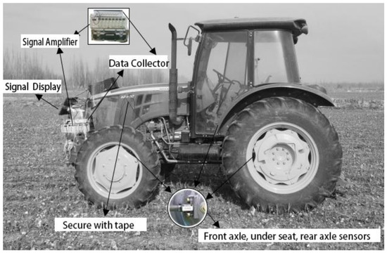
Figure 1. Test site and vehicle.

Table 1. Tractor parameters.

Parameter	Data
Weight	3488 kg
Length	4.372 m
Standard tire pressure for front wheels	240 kPa
Front wheelbase	1.556–1.845 m
Rear wheel standard tire pressure	200 kPa
Rear wheelbase	1.512–1.851 m
Engine rated speed	2300 r/min
Tractor wheelbase	2.23 m

2.1.2. Experimental Site

We conducted experiments in the 21st company of the 9th regiment, Alar, Xinjiang Uygur Autonomous Region. A harvested cotton cultivation field was selected as the experimental site. The soil hammering test and modal analysis were conducted according to the excitation characteristics of road–vehicle interaction [27,28]. The results are shown in Figure 2. The average value of the intrinsic frequency of the 10 groups of soils was 2328.576 Hz, and the damping ratio was 0.1. The soil at the experimental site was sandy.

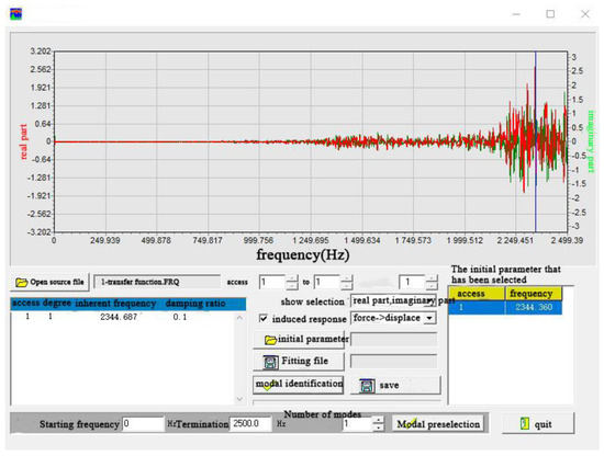
Figure 2. Results of modal analysis of first set of soil hammering tests.

2.1.3. Experimental Protocol

The hardware and virtual instruments used in the experiment are listed in Table 2. We measured the vertical and longitudinal acceleration signals immediately below the center of the front axle, the seat, and the center of the rear axle. The experiments were conducted at different speeds (850, 950, 1050, 1150, and 1250 r/min) and tire pressures (200, 180, 160, 140, and 120 kPa). The experimental steps were as follows: (1) connect the equipment and instruments and fix the tractor front counterweight area while the mainframe is fixed over the front of the tractor; (2) shut off the engine after driving the tractor to the test site and keep the tractor stationary; and (3) start the engine and step on the accelerator until it reaches the expected set speed. The data were collected after the speed was stable and were then saved.

Table 2. Signal acquisition and storage system.

Instrument	Model
Virtual instruments	VibeSys
Acceleration sensor	BZ1123
Integral amplifier	WS-2401
Data collector	WS-5291
Computers	Windows v1.02
Vehicle-mounted correction inverter	TX-1000VA
Portable battery	4 × 12 v
Sampling rate	2000 Hz

The vibration signal was measured by an acceleration sensor and collected by a data acquisition system after amplification by a multichannel charge–voltage amplifier. The air pressure measurement and instrumentation arrangement are shown in Figure 3.

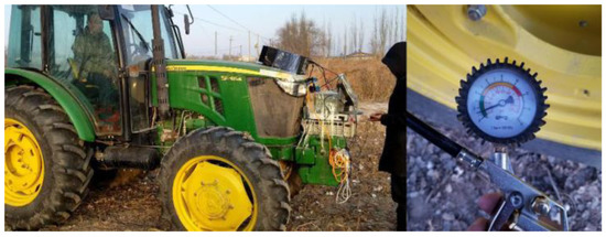
Figure 3. Instrument arrangement and air pressure measurement.

2.2. Feature Extraction and State Recognition Methods

The measured raw signals were decomposed into intrinsic mode functions of different bandwidths using VMD, and the state information of the tractor was estimated using this model. We introduced entropy theory to quantize the model and obtain eigenvectors. The eigenvectors were then input into the classifier, and the state classification model of the tractor was acquired. Finally, by inputting the signal to be recognized into the classifier model, the tractor’s state could be obtained. The vibration signal analysis process is illustrated in Figure 4.

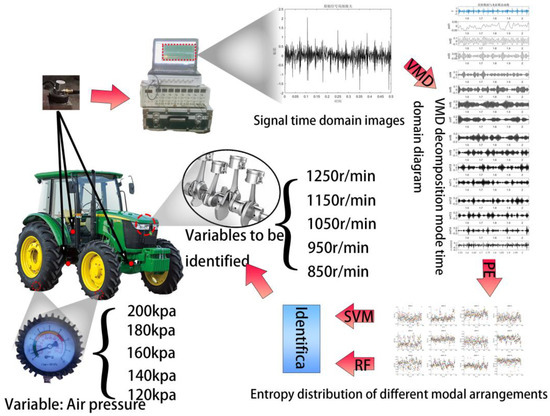
Figure 4. Flowchart of vibration signal analysis.

2.2.1. Variational Mode Decomposition

The VMD algorithm is a collection of components, $u_k$, and the average frequency of each component is ${\omega }_k$.

The steps used to decompose the original signal into K modal components of the VMD are as follows:

• Initialize $\left\{{\widehat{u}}_k^1\right\}$, $\left\{{\widehat{\omega }}_k^1\right\}$, ${\widehat{\lambda }}^1$, $n$ to 0.
• Perform iterative update of ${\widehat{u}}_k$, ${\omega }_k$, $\widehat{\lambda }$ by Equations (1)–(3) and stop when iteration termination condition (4) is satisfied, where ϵ > 0.

  $${\widehat{u}}_k^{n+1}\left(\omega \right)=\frac{\widehat{f}\left(\omega \right)-{{\displaystyle \sum }}_{i<k}{\widehat{u}}_i^n\left(\omega \right)-{{\displaystyle \sum }}_{i>k}{\widehat{u}}_i^n\left(\omega \right)+\frac{{\widehat{\lambda }}^n\left(\omega \right)}{2}}{1+2\alpha {\left(\omega -{\omega }_k^n\right)}^2}$$

  (1)

  $${\omega }_k^{n+1}=\frac{{{\displaystyle \int }}_0^{\infty }\omega {\left|{\widehat{u}}_k^{n+1}\left(\omega \right)\right|}^{2}d\omega }{{{\displaystyle \int }}_0^{\infty }{\left|{\widehat{u}}_k^{n+1}\left(\omega \right)\right|}^{2}d\omega }$$

  (2)

  $${\hat{\lambda }}^{n+1}\left(\omega \right)={\hat{\lambda }}^n\left(\omega \right)+\tau \left(\widehat{f}\left(\omega \right)-{\displaystyle \sum }_k{\widehat{u}}_k^{n+1}\left(\omega \right)\right)$$

  (3)

  $${{\displaystyle \sum }}_k^{}\frac{||{\widehat{u}}_k^{n+1}-{\widehat{u}}_k^n||{}_2^2}{||{\widehat{u}}_k^n||{}_2^2}<ϵ$$

  (4)
• Obtain the K modal components, where $\widehat{f}\left(\omega \right)$ is the result of f(t), which is converted by the Fourier function; α is the penalty factor; λ is the Lagrange multiplier; and ϵ is the loop stop threshold, i.e., the allowed maximum value of the summation of error terms.

2.2.2. Permutation Entropy

Entropy is a measure of the disorder within a system. The more complex the molecules within the system, the higher the entropy, and vice versa. PE was proposed by Bandt et al. [29] and is used to describe the irregularity of time series and complexity of nonlinear systems. Compared with sample entropy and fractal dimension, permutation entropy has the advantages of high computing speed and strong robustness to noise [30,31].

The calculation steps of the PE algorithm are as follows:

1

Reconstruct in phase space the computed time series x(i), i∈(1,N) and obtain a matrix:

$$\left[\begin{array}{cc}\begin{array}{cc}x\left(1\right)\hspace{1em}& x\left(1+\tau \right)\end{array}& \begin{array}{cc}\dots \hspace{1em}& x\left(1+\left(n-1\right)\tau \right)\end{array}\\ \begin{array}{cc}\begin{array}{c}⋮\\ x\left(j\right)\\ \begin{array}{c}⋮\\ x\left(G\right)\end{array}\end{array}& \begin{array}{c}⋮\\ x\left(j+\tau \right)\\ \begin{array}{c}⋮\\ x\left(G+\tau \right)\end{array}\end{array}\end{array}& \begin{array}{cc}\begin{array}{c} \\ \dots \\ \begin{array}{c} \\ \dots \end{array}\end{array}& \begin{array}{c}⋮\\ x\left(j+\left(n-1\right)\tau \right)\\ \begin{array}{c}⋮\\ x\left(G+\left(n-1\right)\tau \right)\end{array}\end{array}\end{array}\end{array}\right]$$

(5)

where n is the embedding dimension (i.e., the length of the intercepted sequence), τ is the delay time (i.e., the interval of sampling points), G is the number of subsequences of the vector space reconstruction, and $G=N-\left(m-1\right)\tau$. The subsequences are:

$$\begin{array}{cc}\begin{array}{cc}[x\left(j\right)& x\left(j+\tau \right)\end{array}& \begin{array}{cc}\dots & x\left(j+\left(n-1\right)\tau \right)\end{array}\end{array}]j\in \left(1,G\right)$$

(6)

2

Transform the obtained G subsequences into permutations by size, considering $n!$ possibilities.

3

Calculate the probability P of each size relationship arrangement:

$$P=c/G$$

(7)

where c is the occurrence frequency of each permutation index.

4

Calculate the information entropy of these probabilities:

$$PE(n)=-{{\displaystyle \sum }}_{n!}Plog\left(P\right)$$

(8)

5

Normalize the PE:

$$PE=PE\left(n\right)/log(n!)$$

(9)

where 0 ≤ PE ≤ 1, and the PE value indicates the disorder level of time series x(i); the higher the PE value, the greater the randomness of x(i); and the smaller the PE value, the stronger the regularity of x(i).

2.2.3. Support Vector Machine

Based on the principle of minimizing structural risk, Vapnik et al. [32] proposed a machine learning algorithm called the support vector machine (SVM). The SVM overcomes many obstacles in artificial neural networks and other methods, such as the difficulty in ensuring the network structure and avoiding overfitting, and can acquire the optimal global solution. It has good generalization performance and unique advantages in solving small samples and in nonlinear and high-dimensional pattern recognition. The essence of the SVM is to find an optimal classification hyperplane that maximizes the sum of the distances from the hyperplane to two types of sample sets. It looks for the best compromise in limited sample information between the complexity of the model’s learning of specific training samples and ability to identify any samples without error, and expects the best generalization ability.

The algorithm can be described as follows:

1

Set the given training sample and expected output.

2

Choose the kernel function K and penalty parameter C to construct the optimization problem.

$$\underset{a}{min}\frac{1}{2}{\displaystyle \sum }_{i=1}^l{\displaystyle \sum }_{j=1}^l{y}_i{y}_j{\alpha }_i{\alpha }_{j}K\left(x_i,x_j\right)-{\displaystyle \sum }_{j=1}^l{\alpha }_j$$

$$s.t.{\displaystyle \sum }_{i=1}^l{y}_i{\alpha }_i=0 0\le {\alpha }_i\le C,i=1, \dots ,l$$

(10)

where the optimal solution is ${\alpha }^{\ast }=\left({\alpha }_1^{\ast },\dots ,{\alpha }_{\mathrm{l}}^{\ast }\right)$.

3

Choose a positive component $b^{\ast }$ from ${\alpha }^{\ast }$ that is less than C.

$$b^{\ast }=y_i-{\displaystyle \sum }_{i=1}^l{y}_i{\alpha }_i^{\ast }K\left(x_i,x_j\right)$$

(11)

4

Find the decision function.

$$f\left(x\right)=\mathrm{sgn}\left[{\displaystyle \sum }_{i=1}^{\mathrm{l}}{y}_i{\alpha }_i^{\ast }K\left(x_i,x\right)+b^{\ast }\right]$$

(12)

The SVM identification steps are shown in Figure 5.

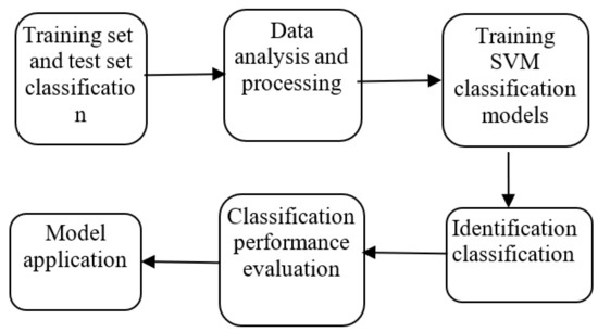
Figure 5. Flowchart of support vector machine classification.

2.2.4. Random Forest

Random forest (RF) is a statistical learning theory proposed by Breiman [33]. The bootstrap resampling method extracts multiple samples from an original sample. Decision tree modeling is carried out for each bootstrap sample, and the final prediction result is acquired by voting combined with the prediction of multiple decision trees. The specific classification mode is as follows: Each decision tree in the forest produces a classification result for the feature matrix consisting of the statistical proportion of each category in the classification results, and the higher proportion is determined as the final classification result. The final classification result is shown in (13):

$$H\left(x\right)=arg \underset{Y}{max}{\displaystyle \sum }_{i=1}^{n}I\left(h_i\left(x\right)=Y\right)$$

(13)

where H(x) is the final classification result, $I\left(h_i\left(x\right)=Y\right)$ is the indicative function, $h_{\mathrm{i}}\left(x\right)$ is the decision tree classification result, and Y is the output variable.

This method has high prediction accuracy and good tolerance for outliers and noise; is not prone to overfitting; and has a wide range of applications in medicine, bioinformatics, and management.

2.3. Tractor Condition Identification Method

Compared with the number of modes and penalty factors, the fidelity coefficient and discriminant accuracy have less influence on the decomposition effect. Therefore, in this study we discuss the number of modes and penalty factors.

The K value is estimated according to the wave number represented by log–log coordinates in the frequency domain of the vibration signal, and its rationality is verified by the center frequency of different K values. To avoid the phenomenon of VMD frequency mixing, we considered frequency points with similar wave peaks as the decomposition number. The convergent curve of the center frequency of each model was calculated to avoid model aliasing. Subsequently, the correlation coefficients of each model and the original signal were calculated to prevent excessive decomposition. Finally, the optimal decomposition quantity, K, was confirmed.

The penalty factor was introduced to convert the constrained variational problem into an unconstrained variational problem. This mainly affected the bandwidth of each mode after decomposition and the convergence speed during the operation of the VMD program. When the penalty factor was 2000, the VMD exhibited strong adaptability by avoiding modal mixing and ensuring convergence speed. The expression of the log–log coordinates in the frequency domain of the vibration signal when the tire pressure was 200 kPa and the speed was 850 rpm is shown in Figure 6.

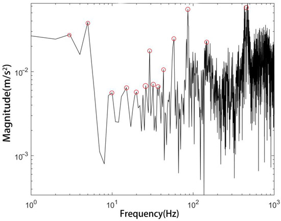
Figure 6. Vibration signal frequency domain double-logarithmic coordinates.

As shown in Figure 6, there were 14 distinct peaks in the log–log coordinates in the frequency domain of the vibration signal. The center frequencies of the modal components at different K values after the vibration signal was decomposed by VMD are presented in Table 3. As shown in Table 3, the number of VMD iterations increased by more than 198% when K was 15 and 16 compared with when it was 14, and the running time of the algorithm was greatly extended. When K was equal to 14, the center frequency interval was more uniform; therefore, the decomposition effect was more ideal.

Table 3. Center frequency and number of iterations corresponding to different K values.

K	N	Center Frequency of Each Mode (Hz)
1	17	92
2	18	90	458
3	86	90	457	792
4	111	90	433	474	794
5	61	82	157	457	666	815
6	107	7	94	432	473	671	817
7	115	7	94	432	473	654	770	858
8	54	6	92	265	433	473	654	771	858
9	130	6	92	264	432	472	600	695	786	866
10	169	5	86	156	355	434	472	602	697	787	867
11	152	5	86	154	285	433	472	594	681	774	849	948
12	107	5	86	153	264	365	434	472	596	683	775	849	948
13	93	5	86	153	264	364	434	472	584	658	722	791	856	952
14	146	5	86	153	263	362	433	466	495	591	660	724	792	857	952
15	436	5	86	153	263	362	433	466	494	589	657	713	770	817	868	957
16	500	5	86	153	261	355	416	437	467	497	590	657	714	770	817	868	957

To avoid excessive decomposition, the correlation coefficient ρ was used to evaluate the correlation between the original signal and each component. The calculation is shown in (14), where $\tilde{f}$ is the eigenmodal function, $f$ is the original signal, $Cov\left(\tilde{f},f\right)$ is the covariance of $\tilde{f}$ and f, $\sqrt{D\left(\tilde{f}\right)}$ is the standard deviation of the Feige modular function, and $\sqrt{D\left(f\right)}$ is the standard deviation of the original signal.

$$\rho =\frac{Cov\left(\tilde{f},f\right)}{\sqrt{D\left(\tilde{f}\right)}\sqrt{D\left(f\right)}}$$

(14)

Three measurement points were considered, and each one was measured in two directions; thus, there were six data groups in total. Ten vibration signals were randomly selected under different working conditions to calculate the VMD. The results in Table 4 show that the correlation coefficient of each mode and the original signal and the mean variance of each group were less than 0.01. S1, S2, S3, S4, S5, and S6 are the vertical signal at the seat, the longitudinal signal at the seat, the vertical signal at the front axle, the longitudinal signal at the rear axle, the longitudinal signal at the rear axle, and the longitudinal signal at the rear axle, respectively. Table 4 also shows that all correlation coefficients of each mode and the original signal were significant at more than 10%, and the correlation coefficient had apparent irrelevance (i.e., recognizability), thereby assuring mode identification. In this study, K = 14, and the images of eigenmode functions after signal decomposition are shown in Figure 7. As shown in the figure, the original signal was decomposed into 14 IMFs and one residual by VMD, and the frequency information of the different modes shows significant variability. The frequency increased sequentially from the first to the 14th eigenmode function.

Table 4. Mean values of correlation coefficients of modes and original signal for 10 sets of data randomly selected for each working condition (%).

K	1	2	3	4	5	6	7	8	9	10	11	12	13	14	More than One Item
S1	30	36	37	42	34	25	23	22	22	25	25	28	31	31	70
S2	14	17	17	18	28	41	49	55	36	30	25	18	15	12	57	10–20
S3	35	23	20	21	19	21	20	21	25	35	42	44	32	31	63	20–30
S4	31	31	39	49	43	33	28	21	19	20	21	23	20	22	65	30–40
S5	44	20	18	23	29	21	18	25	42	37	32	32	29	21	58	40–50
S6	37	28	24	18	27	31	39	47	40	18	19	21	17	11	52	>50

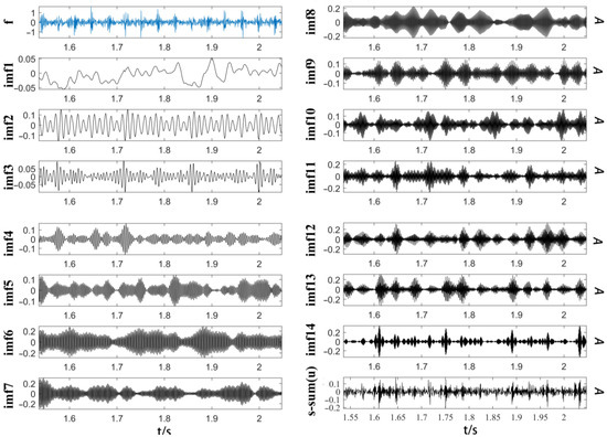
Figure 7. Raw data with eigenmode function and residual term time-domain alignment entropy parameter selection.

The embedding dimension (alignment entropy order) m, delay time τ, and time series length N should be set to calculate PE. The alignment entropy of the signal was slightly affected when τ varied from 1 to 6. Therefore, we set τ as 1.

When m equals 1 or 2, the number of reconstructed vectors in the algorithm is small; when m is greater than 7, the phase space reconstruction makes the time series homogeneous, which cannot accurately reflect small changes in the time series. Therefore, embedding dimension m typically ranges from 3 to 7. Cao et al. [34] found that alignment entropy best characterized the changing characteristics of the time series when m was 5–7. Therefore, m = 6 was set.

The PE values for different signal lengths at different m values are shown in Figure 8. The signal lengths were 256, 512, 1024, 2048, and 4096 points. Figure 8 shows that when m < 6, the entropy of the arrangement of signals of different lengths varied less and was not easily distinguished; when m = 6, the signals could be distinguished.

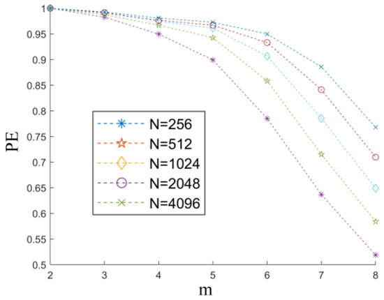
Figure 8. Alignment entropy of vibration signals of various lengths.

Figure 9 shows the variation curves of alignment entropy for different data lengths under the condition of 200 kPa tire pressure and 850 r/min speed. The alignment entropy tended to stabilize when the data length was >1000. Considering the computational cost and stability, we set the data length to 1024.

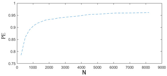
Figure 9. Alignment entropy variation curves for different signal lengths.

3. Results

We conducted experiments under 25 different working conditions. We measured the vibration signals of the tractor at five speeds with five tire pressures. For each condition, the vertical and longitudinal acceleration signals were measured. The measurement points were set at the center of the front axle, directly below the seat in the cabin, and directly below the center of the rear axle. We chose 38 groups of data for each working condition, and the data size for each group was 1024. In this section, 5700 groups of data are classified.

3.1. State Recognition Based on SVM

Each dataset contained signals in one direction for one measurement point, and each set was decomposed by VMD. Fourteen modal components and one residual term constituted the sample. Therefore, we acquired 950 × 15 permutation entropy values; that is, 950 feature vectors containing 15 attributes. A total of 800 feature vectors were used as the training set, which was input into the SVM classifier for training. The remaining 150 samples were used as test samples. Parameters c and g were determined by K-fold cross-validation (K-CV), which can effectively avoid the occurrence of over- or under-learning. The training sets were subdivided into training and validation samples, and the training samples were used to train the model. The validation samples were used to verify the model and acquire the performance index of the classifier, which was evaluated based on the accuracy of the classification. Figure 10 shows a contour chart of the iterative process of selecting c and g. As shown in the figure, the vertical vibration signals were sparse for the best parameter selection of the three measurement points. The results of the model training for the best performance were lower than those for the longitudinal vibration signal.

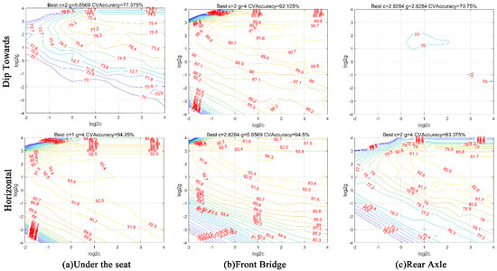
Figure 10. SVM cross-validation parameter selection results.

The 150 feature vectors of the test set of vibration signals measured under different operating conditions were input into the trained SVM for tractor engine state recognition. The recognition accuracy values are listed in Table 5.

Table 5. Recognition accuracy of SVM (%).

Direction	Seats	Front Bridge	Rear Axle	Average Value
Vertical	82.66	95.33	75.33	84.44
Crosswise	97.33	96.66	88	93.99
Average value	89.99	95.99	81.66

3.2. State Recognition Based on Random Forest

A total of 800 feature vectors were randomly selected from a set of 950 feature vectors to train the decision tree. The remaining 150 feature vectors were input into the model to perform state recognition after the classification model was obtained. The confusion matrix is shown in Figure 11. The horizontal coordinate represents the attribute’s practical category, and the vertical coordinate represents the attribute’s predicted category. The numbers 1–5 represent the five engine speed conditions. Figure 11a shows the confusion matrix for the identification of vibration signal properties under the seat. Figure 11b shows the confusion matrix for the identification of vibration signal properties at the front axle. Figure 11c shows the confusion matrix for the identification of vibration signal properties at the rear axle. The last column of each confusion matrix indicates the related predicted category’s recognition accuracy and error rate, and the last row indicates the related actual sample’s recognition accuracy and error rate.

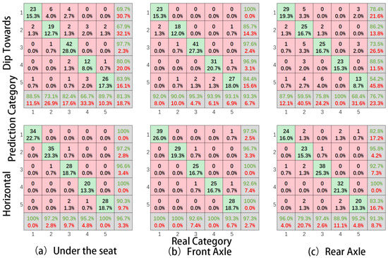
Figure 11. Random forest confusion matrices.

The diagonal line of the matrix shows the number and proportion of samples correctly classified by the model, and the last cell of the diagonal line indicates the classification accuracy of the model. The results show that the recognition accuracy is significantly better for the longitudinal vibration signal than the transverse vibration signal and decreases for the front axle, under the seat, and rear axle vibration signal in turn. The final recognition accuracy results are presented in Table 6.

Table 6. Recognition accuracy of random forest (%).

Direction	Seats	Front Bridge	Rear Axle	Average Value
Vertical	81.33	93.33	76.67	83.77
Crosswise	96.67	97.33	91.33	95.11
Average value	89	95.33	84

3.3. State Recognition Based on EMD and SVM

In this section, EMD is used to analyze the tractor vibration signal, and the analysis results are shown in Figure 12. After calculating the correlation between IMF and the original signal and excluding the over-decomposed signal, the correlation coefficient between the IMF and the original signal after the decomposition of 10 groups of signals is randomly selected, as shown in Figure 13a. It can be seen from the figure that after decomposition to IMF7, the correlation coefficient with the original signal drops below 10%, and the correlation with the original signal is small. To avoid calculation waste caused by excessive decomposition, only the first six IMFs are identified. Figure 13b shows the correlation coefficient of the IMF obtained from VMD. It can be seen from the figure that the correlation between the 14 intrinsic mode functions of variational mode decomposition and the original signal are all above 10%, which proves that VMD can effectively round out the attribute table of vibration signals, thus improving the accuracy of state recognition. The support vector machine (SVM) was used to identify the decomposed eigenmode function quantified by permutation entropy. The results show that the recognition accuracy of the longitudinal vibration signal of the front bridge was the highest at 62%, as shown in Figure 14. The superiority of the proposed method is proved by comparing the results.

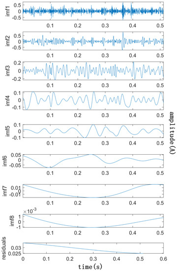
Figure 12. Time-domain diagram of EMD eigenmodes.

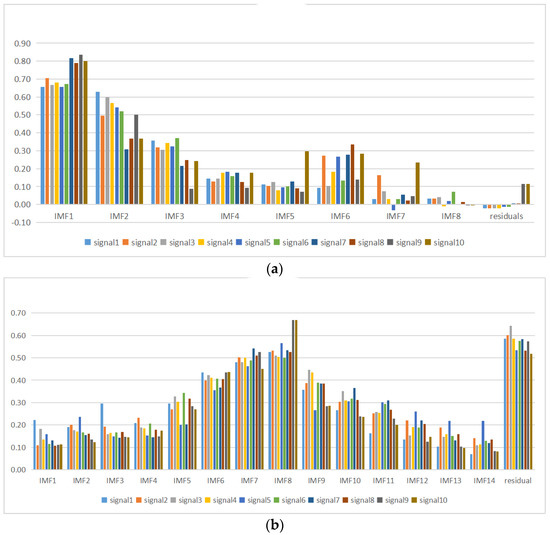
Figure 13. Degree of correlation between (a) IMF of EMD and original signal and (b) IMF of VMD and original signal.

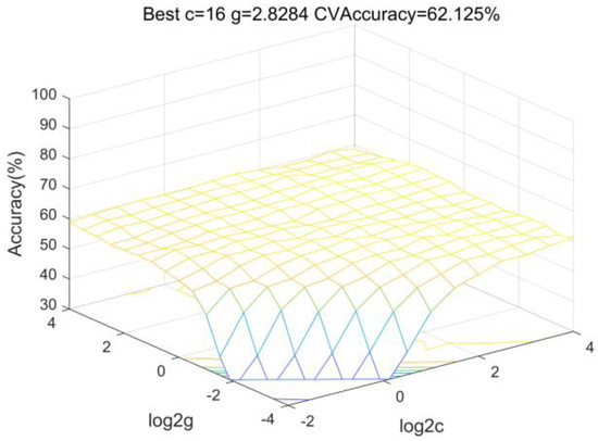
Figure 14. Identification results of support vector machine based on EMD.

3.4. State Recognition Based on VMD and Backpropagation

In this section, the PE value of the IMF obtained from VMD is used as the attribute value of the signal to train backpropagation to get the classification model. For this process, 15 neurons were set in the input layer according to the number of IMFs, 25 neurons were set in the hidden layer, 5 neurons were set in the output layer according to the 5 speed levels, and the number of optimization iterations was set to 10. The classification results are shown in Table 7. The optimal classification result is the vertical vibration signal of the front bridge position, as shown in Figure 15a. Figure 15b shows the total deviation of cyclic iterative training data. It is proved that the classification accuracy is lower for backpropagation than for the support vector machine.

Table 7. Recognition accuracy of backpropagation (%).

Direction	Seats	Front Bridge	Rear Axle	Average Value
Vertical	67.33	84.67	60.00	70.66
Crosswise	83.33	82.67	74.67	80.22
Average value	75.33	83.67	67.33

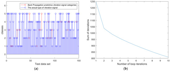
Figure 15. (a) Identification results of longitudinal vibration signal of front axle; (b) deviation sum of iteration training data.

4. Discussion

This study proposes a tractor state identification method based on variational mode decomposition and alignment entropy under different engine speeds and tire pressures when driving. The vibration signal measured by the tractor during the operation is decomposed by VMD. The modal components of each order are then calculated by ranking the entropy and input in the SVM training as feature vectors in order to obtain a classification model and identify the tractor running signal.

The results of this study indicate the following:

The application of VMD in tractor engine state identification can effectively decompose the signal into modal components within a specific bandwidth. The different signals are characterized by VMD, which can provide decomposition data without modal confounding for subsequent feature extraction and state identification. Alignment entropy can effectively represent the time variation of the modal components of VMD. The experimental results prove that the vibration signals during tractor operation under various conditions were strongly identifiable through alignment entropy to characterize the time-series variation. The applicability of VMD to the decomposition of vibration signals in the agricultural operating environment described in this paper was demonstrated by a comparative study of EMD and VMD. A comparative study of the recognition effects of support vector machines and random forests over BP neural networks demonstrates the superiority of traditional machine learning recognition when using a small sample.

This study explored the distribution pattern of the effective signal using the distribution distance of the sensor. We analyzed the tractor’s vertical and longitudinal acceleration signals and found that the longitudinal signal was significantly better for discriminating tractor engine speed. The closer to the engine, the higher the recognition accuracy, as analyzed by the recognition of different measurement points relative to the engine.

In this paper, we propose a method to simulate the conditions of different types of agricultural practices by changing the tractor’s tire pressure in order to address the problem that it is difficult to quantify the regularity of the working surface of agricultural machinery. The variability of the identification results under different tire pressure conditions proves the effectiveness of the method. The results of the experimental analysis prove that the vibration signal can express the engine speed working condition more accurately under different ground surface driving conditions of the tractor.

References

- Martin, P.L.; Olmstead, A.L. The Agricultural Mechanization Controversy. Science 1985, 1, 601–605. [Google Scholar] [CrossRef]
- Daum, T.; Birner, R. Agricultural mechanization in Africa: Myths, realities and an emerging research agenda. Glob. Food Secur. 2020, 26, 100393. [Google Scholar] [CrossRef]
- Yang, W.X.; Zimroz, R.; Papaelias, M. Advances in Machine Condition Monitoring and Fault Diagnosis. Electronics 2022, 11, 1563. [Google Scholar] [CrossRef]
- Yule, I.J.; Kohnen, G.; Nowak, M. A tractor performance monitor with DGPS capability. Comput. Electron. Agric. 1999, 23, 155–174. [Google Scholar] [CrossRef]
- Delgado-Arredondo, P.A.; Morinigo-Sotelo, D.; Osornio-Rios, R.A.; Avina-Cervantes, J.G.; Rostro-Gonzalez, H.; Romero-Troncoso, R.J. Methodology for fault detection in induction motors via sound and vibration signals. Mech. Syst. Signal Process. 2017, 83, 568–589. [Google Scholar] [CrossRef]
- Qiang, W.; Peilin, Z.; Chen, M.; Huaiguang, W.; Cheng, W. Multi-task Bayesian compressive sensing for vibration signals in diesel engine health monitoring. Measurement 2018, 136, 625–635. [Google Scholar] [CrossRef]
- Rahman, A.; Hoque, M.E.; Rashid, F.; Alam, F.; Ahmed, M.M. Health Condition Monitoring and Control of Vibrations of a Rotating System through Vibration Analysis. J. Sens. 2022, 4281596. [Google Scholar] [CrossRef]
- Nguyen, V.N.; Matsuo, T.; Inaba, S.; Koumoto, T. Experimental analysis of vertical soil reaction and soil stress distribution under off-road tires. J. Terramech. 2008, 45, 25–44. [Google Scholar] [CrossRef]
- Hosseinpour-Zarnaq, M.; Omid, M.; Biabani-Aghdam, E. Fault diagnosis of tractor auxiliary gearbox using vibration analysis and random forest classifier. Inf. Process. Agric. 2022, 9, 60–67. [Google Scholar] [CrossRef]
- Bahrami, M.; Javadikia, H.; Ebrahimi, E. Intelligent Prediction of Fault Severity of Tractor’s Gearbox by Time-domain and Frequency-domain (FFT phase angle and PSD) Statistics Analysis and ANFIS. J. Mech. Eng. 2017, 47, 51–61. [Google Scholar] [CrossRef]
- Sun, M.L.; Lu, C.H.; Liu, Z.; Shen, C.R.; Chen, H.; Sun, Y. Response Synthesizing Based on Global Transmissibility Direct Transmissibility Method: A Case Numerical and Experimental Study. J. Vib. Eng. Technol. 2022. [Google Scholar] [CrossRef]
- Li, D.; Zheng, Y.; Zhao, W. Fault Analysis System for Agricultural Machinery Based on Big Data. IEEE Access 2019, 7, 99136–99151. [Google Scholar] [CrossRef]
- Zheng, E.; Cui, S.; Yang, Y.Z.; Xue, J.L.; Zhu, Y.; Lin, X.Z. Simulation of the Vibration Characteristics for Agricultural Wheeled Tractor with Implement and Front Axle Hydropneumatic Suspension. Shock. Vib. 2019, 2019, 9135412. [Google Scholar] [CrossRef]
- Deboli, R.; Calvo, A.; Preti, C. Whole-body vibration: Measurement of horizontal and vertical transmissibility of an agricultural tractor seat. Int. J. Ind. Ergon. 2017, 58, 69–78. [Google Scholar] [CrossRef]
- Hajnayeb, A.; Fernando, J.S.; Sun, Q. Effects of vehicle driveline parameters and clutch judder on gearbox vibrations. Proc. Inst. Mech. Eng. Part D J. Automob. Eng. 2021, 236, 84–98. [Google Scholar] [CrossRef]
- Chen, P.S.; Xu, L.Y.; Tang, Q.S.; Shang, L.L.; Liu, W. Research on prediction model of tractor sound quality based on genetic algorithm. Appl. Acoust. 2022, 185, 108411. [Google Scholar] [CrossRef]
- Migal, V.; Arahun, S.; Shuliak, M.; Huatov, A.; Trunova, I.; Shevchenko, I. Assessing design and manufacturing quality of tractor gearboxes by their vibration characteristics. J. Vib. Control 2022, 1–11. [Google Scholar] [CrossRef]
- Phromjan, J.; Suvanjumrat, C. Vibration effect of two different tires on baggage towing tractors. J. Mech. Sci. Technol. 2018, 32, 1539–1548. [Google Scholar] [CrossRef]
- Liu, C.; Cheng, G.; Chen, X.H.; Pang, Y.S. Planetary gears feature extraction and fault diagnosis method based on VMD and CNN. Sensors 2018, 18, 1523. [Google Scholar] [CrossRef]
- Dragomiretskiy, K.; Zosso, D. Variational Mode Decomposition. IEEE Trans. Signal Process. 2014, 62, 531–545. [Google Scholar] [CrossRef]
- Chen, S.Q.; Yang, Y.; Dong, X.J.; Xing, G.P.; Peng, Z.K.; Zhang, W.M. Warped Variational Mode Decomposition With Application to Vibration Signals of Varying-Speed Rotating Machineries. IEEE Trans. Instrum. Meas. 2019, 68, 2755–2767. [Google Scholar] [CrossRef]
- Miao, Y.H.; Zhang, B.Y.; Li, C.H.; Lin, J.; Zhang, D.Y. Feature Mode Decomposition: New Decomposition Theory for Rotating Machinery Fault Diagnosis. IEEE Trans. Ind. Electron. 2023, 70, 1949–1960. [Google Scholar] [CrossRef]
- Wang, X.B.; Yang, Z.X.; Yan, X.A. Novel Particle Swarm Optimization-Based Variational Mode Decomposition Method for the Fault Diagnosis of Complex Rotating Machinery. IEEE/ASME Trans. Mechatron. 2018, 23, 68–79. [Google Scholar] [CrossRef]
- Feng, Z.P.; Zhang, D.; Zuo, M.J. Adaptive Mode Decomposition Methods and Their Applications in Signal Analysis for Machinery Fault Diagnosis: A Review With Examples. IEEE Access 2017, 5, 24301–24331. [Google Scholar] [CrossRef]
- Cao, P.P.; Wang, H.L.; Zhou, K.J. Multichannel Signal Denoising Using Multivariate Variational Mode Decomposition With Subspace Projection. IEEE Access 2020, 8, 74039–74047. [Google Scholar] [CrossRef]
- Zhang, C.; Zhang, Y.B.; Hu, C.X.; Liu, Z.B.; Cheng, L.Y.; Zhou, Y. A Novel Intelligent Fault Diagnosis Method Based on Variational Mode Decomposition and Ensemble Deep Belief Network. IEEE Access 2020, 8, 36293–36312. [Google Scholar] [CrossRef]
- Cheng, Y.S.; Li, X.Q.; Sun, S.S. A new method for expression and classification of long wave road surface unevenness in field. J. Vib. Shock. 2022, 41, 180–188. [Google Scholar]
- Cheng, Y.S.; Li, X.Q.; Man, X.L.; Fan, F.F.; Li, Z.X. Perceiving Excitation Characteristics from Interactions between Field Road and Vehicle via Vibration Sensing. Hindawi 2021, 5548725. [Google Scholar] [CrossRef]
- Bandt, C.; Pompe, B. Permutation entropy: A natural complexity measure for time series. Phys. Rev. Lett. 2002, 88, 174102. [Google Scholar] [CrossRef]
- Guo, Y.F.; Zhang, Z.S. Generalized Variational Mode Decomposition: A Multiscale and Fixed-Frequency Decomposition Algorithm. IEEE Trans. Instrum. Meas. 2021, 70, 1–13. [Google Scholar] [CrossRef]
- Chen, X.J.; Yang, Y.M.; Cui, Z.X.; Shen, J. Wavelet Denoising for the Vibration Signals of Wind Turbines Based on Variational Mode Decomposition and Multiscale Permutation Entropy. IEEE Access 2020, 8, 40347–40356. [Google Scholar] [CrossRef]
- Cortes, C.; Vapnik, V. Support-Vector Networks. Mach. Learn. 1995, 20, 273–297. [Google Scholar] [CrossRef]
- Breiman, L. Random Forests. Mach. Learn. 2001, 45, 5–32. [Google Scholar] [CrossRef]
- Cao, Y.H.; Tung, W.W.; Gao, J.B.; Protopopescu, V.A.; Hively, L.M. Detecting dynamical changes in time series using the permutation. Phys. Rev. E 2004, 70, 046217. [Google Scholar] [CrossRef] [PubMed]
Disclaimer/Publisher’s Note: The statements, opinions and data contained in all publications are solely those of the individual author(s) and contributor(s) and not of MDPI and/or the editor(s). MDPI and/or the editor(s) disclaim responsibility for any injury to people or property resulting from any ideas, methods, instructions or products referred to in the content. |
© 2023 by the authors. Licensee MDPI, Basel, Switzerland. This article is an open access article distributed under the terms and conditions of the Creative Commons Attribution (CC BY) license (https://creativecommons.org/licenses/by/4.0/).