Research of Carbon Emission Prediction: An Oscillatory Particle Swarm Optimization for Long Short-Term Memory

Abstract

Carbon emissions play a significant role in shaping social policy-making, industrial planning, and other critical areas. Recurrent neural networks (RNNs) serve as the major choice for carbon emission prediction. However, year-frequency carbon emission data always results in overfitting during RNN training. To address this issue, we propose a novel model that combines oscillatory particle swarm optimization (OPSO) with long short-term memory (LSTM). OPSO is employed to fine-tune the hyperparameters of LSTM, utilizing an oscillatory strategy to effectively mitigate overfitting and consequently improve the accuracy of the LSTM model. In validation tests, real data from Hainan Province, encompassing diverse dimensions such as gross domestic product, forest area, and ten other relevant factors, are used. Standard LSTM and PSO-LSTM are selected in the control group. The mean absolute error (MAE), root mean square error (RMSE), and mean absolute percentage error (MAPE) are used to evaluate the performance of these methods. In the test dataset, the MAE of OPSO-LSTM is 117.708, 65.72% better than LSTM and 29.48% better than PSO-LSTM. The RMSE of OPSO-LSTM is 149.939, 68.52% better than LSTM and 41.90% better than PSO-LSTM. The MAPE of OPSO-LSTM is 0.017, 65.31% better than LSTM, 29.17% better than PSO-LSTM. The experimental results prove that OPSO-LSTM can provide reliable predictions for carbon emissions.

1. Introduction

Carbon emission projections (CEPs) are pivotal in achieving dual carbon goals, and they will play a critical role in driving future low-carbon and environmentally friendly development within the local economy and society. CEPs also serve as a valuable guide for businesses and investors operating in energy, transportation, manufacturing, and various other sectors. Foreseeing future carbon emission levels enables companies and investors to evaluate the environmental risks and opportunities associated with different investment projects and determine the strategic direction for sustainable development. Additionally, some financial institutions and investors utilize carbon emissions projections to assess the carbon footprint and climate-related risks within their portfolios.

Lastly, carbon emission projections empower companies and organizations to more effectively manage their resource and energy consumption. By gaining insight into future carbon emissions, companies can take proactive measures to reduce energy consumption, lower carbon emissions, enhance resource efficiency, and develop sustainable strategies for their business operations and supply chain management.

Recurrent neural networks (RNNs) are a popular choice for time-series data prediction tasks. They are well suited for this purpose due to their inherent ability to process sequential data while maintaining a memory of past information. RNNs excel in capturing temporal dependencies and patterns within time series, making them effective for tasks like stock price forecasting, weather prediction, and natural language processing.

However, traditional RNN algorithms applied to carbon emissions prediction tasks can face several challenges. Firstly, they struggle with capturing long-term dependencies in the data, hindering their ability to model extended trends and seasonal patterns. Secondly, these models are prone to overfitting, especially when dealing with complex and high-dimensional datasets. Additionally, selecting appropriate hyperparameters, such as the size of hidden layers and learning rates, can be a challenging task. Lastly, RNN models may be susceptible to getting stuck in local minima during training, making it difficult to achieve global optimization and accurate predictions.

To address these challenges and improve the accuracy of carbon emission prediction, we propose a novel oscillatory particle swarm optimization (OPSO)-based long short-term Memory (LSTM) model. Specifically, this paper makes several key contributions:

Firstly, we introduce the concept of OPSO. OPSO employs an oscillatory strategy to enhance the search capability of traditional particle swarm optimization (PSO) in high-dimensional spaces.

Secondly, we integrate OPSO with the conventional LSTM model. OPSO is employed to fine-tune the hyperparameters of LSTM. Our method effectively addresses issues associated with PSO, such as limited search range, susceptibility to early local optima, and reduced search accuracy in later stages. By combining OPSO with LSTM, we optimize LSTM’s parameters, thereby improving its efficiency when confronted with a larger number of network layers.

The rest of this paper is organized as follows: in Section 2, recent works related to carbon emission are presented; in Section 3, the structure and process of the proposed method are introduced; in Section 4, experimental details and results are presented; in Section 5, the conclusion of this work is presented.

2. Related Work

Research related to carbon emissions encompasses a wide range of topics, such as carbon emission measurement and monitoring, strategies and technologies for carbon reduction, assessments of climate change impacts, the functioning of carbon markets, mechanisms for carbon pricing, and various policy and regulatory measures. Abeydeera [1] examined the global literature on carbon emissions. The findings reveal a clear and consistent upward trajectory in the number of publications within the field of carbon emissions research.

Comparing regional carbon emission differences in China, in 2020, Wang [2] measured the total amount and intensity of China’s agricultural carbon emissions and compared the regional differences in China’s agricultural carbon emissions using the coefficient of variation method and the Theil index method. In 2021, Jin [3] collected and analyzed data on carbon emissions from China’s provinces from 1999 to 2019, and the results show that the per-capita carbon emissions of residents in northern China are significantly higher than those in southern China, and that the rate of carbon emissions continues to increase. Gao [4] constructed a non-competitive input–output model to measure the embodied carbon emissions of 28 industry sectors in China from 2005 to 2017. In 2022, Cai [5] used carbon emissions data to map inter-city linkages and build networks that have substantial implications for China’s inter-city carbon emission linkage network.

Carbon emissions are influenced by various aspects, in 2019, Klc [6] investigated whether corporate governance characteristics influence voluntary disclosure of carbon emissions. The results indicate that entities with a higher number of independent directors on their boards are more likely to respond to carbon disclosure projects. Waheed [7] stated that carbon emissions are also related to the level of development of the country. In 2021, Lee [8] examined the relationship between carbon emissions, carbon disclosure, and firm value in Korean companies and found a significant positive correlation between carbon emissions and firm value in Chaebol affiliates. In 2022, Alam [9] examined whether corporate cash holdings affect CO₂ emissions. Companies with higher corporate cash holdings were found to have lower carbon emissions. Bai [10] found that green finance has an effect on carbon emissions based on Hansen’s threshold regression model. In 2023, Ott [11] broke down carbon emissions into expected and unexpected components and analyzed the link between these components and the value of the company. The results show that, on average, investors place a high value on both components. In addition, the local carbon emissions trading policy (CETP) also has an impact on it. Chen [12] analyzed panel data for 282 prefecture-level and above cities in China from 2007 to 2017, and found that CETP can significantly improve the efficiency of carbon emissions in pilot cities.

To reduce carbon emissions, Mou [13] proposed a new adaptive dynamic wireless charging system that enables mobile electric vehicles to be powered by renewable wind energy. Many other studies have been conducted on the subject. Ahvar [14] proposed a novel placement method that takes into account geographic location, energy costs, and other factors, allowing for more logical placement of edge cloud applications to optimize energy costs and carbon emissions.

There are many scholars around the world who have used various models to study how to predict carbon emissions and how to make other predictions. For instance, Zhou [15] built multiple one-step predictors to analyze and predict carbon prices based on fully ensemble empirical model decomposition with adaptive noise (CEEMDAN) and long short-term memory (LSTM) recurrent neural networks. Kong [16] proposed a new type of short-term carbon emission forecasting model, EVPL, which can further improve the accuracy of forecasting. Hu [17] proposed ROGM-AFSA-GVM to predict the non-linear law of ROS. Wang [18] used the SSA-LSTM algorithm to develop a carbon emission regression prediction model for coal-fired power plants. Gao [19] proposed the FGRM(1,1) model to obtain the best fractional order, which has better estimation and has shown efficiency in short-term carbon emission projections. Wang [20] established the spatial gray model SGM(1,1,m) and implemented the gray model to model spatial data. Cai [21] constructed an SVR model for predicting carbon emissions from agroforestry ecosystems and solved the regression function for sample data. Kong [22] proposed a prediction model using a combination of ICEEMDAN, PACF, and ReliefF called ISSA-ELM. The results show that the proposed two-stage feature selection method can further improve prediction accuracy. Huang [23] presented an SVR machine prediction model. The results show that the SVR model for solving complex non-linear problems can achieve more satisfactory prediction results with the training of LSTM. Zhao [24] proposed a long short-term memory network optimized by a sparrow search algorithm and applied it to carbon emission prediction in the Yellow River Basin. Lu [25] proposed a three-layer PNN to learn the features of collected data and to infer traffic carbon emissions.

Greff [26] conducted a large-scale analysis of eight LSTM variants for three representative tasks, showing that none of the variants provide a significant improvement on the standard LSTM architecture and demonstrating that the forgetting gate and output activation function are its most critical components. Abbasimehr [27] proposed a demand forecasting method based on a multilayer LSTM network. The method aims to accurately predict highly volatile demand data in a competitive business environment. The proposed method automatically selects the best forecasting model by exploring various combinations of LSTM hyperparameters using a grid search method. Zhao [28] made significant strides in the field of carbon emissions prediction through the introduction of the support vector regression LSTM model, providing robust support and guidance for addressing climate change and carbon emission management.

At the same time, others have used algorithms to solve such problems. Various improved algorithms based on PSO show different optimization capabilities and effects. Guo [29] proposed PBBPSO to balance exploration and development. Tian [30] proposed an electronic transition-based BBPSO for high-dimensional problems. Guo [31] proposed the TBBPSO algorithm, which enhances the local minimum escape capability of the proposed method. Guo [32] proposed BPSO-CM, where particle swarms are given enhanced global search capabilities. Xiao [33] proposed TMBPSO, where the particle swarm is endowed with the ability to self-correct. Li [34] proposed an optimized VMD and ELM, the ISGSP, to construct a decomposition–prediction to forecast carbon emissions. Guo [35] proposed FHBBPSO, and the results show that FHBBPSO is a highly competitive optimization algorithm for single-objective functions.

3. Materials and Methods

Traditional RNN models demand substantial training data to guarantee model accuracy. Nevertheless, carbon emission datasets typically consist of only 30 annual data points, rendering traditional RNNs susceptible to overfitting during training. In this part, we introduce a novel solution to address this challenge by employing the oscillating particle swarm algorithm. Additionally, the model presented in this article offers the capability to monitor statistical outcomes from relevant agencies and even provide feedback on unusual data patterns, enhancing its versatility and practicality.

3.1. Long Short-Term Memory

The long short-term memory (LSTM) network is a special version of the traditional recurrent neural network (RNN). LSTM effectively solves the problem of gradient vanishing and gradient explosion in long series prediction. Compared with the traditional neural network, LSTM relies on the gate mechanism. The LSTM through the gate mechanism controls the flow of information input and output. The cell unit form of LSTM and the network structure of LSTM are shown in Figure 1. In Figure 1, the yellow part represents the fully connected layer, the purple part represents the LSTM layer, and the yellow part represents features.

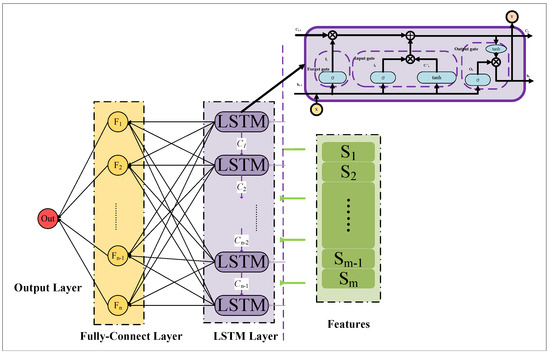
Figure 1. The cell unit form of LSTM and the network structure of LSTM. Source: own creation.

The gate mechanisms are proposed for LSTM, including the forget gate, the input gate, and the output gate. At a specific time, the cell input of LSTM consists of the sequence input $x_t$, the state of the previous hidden layer $h_{t-1}$, and the state of the previous cell $C_{t-1}$. In the first step, the forget gate forgets useless input information by Equations (1) and (2).

$$v_t=[h_{t-1},x_t]$$

(1)

$$f_t=\sigma (W_f·v_t+b_f)$$

(2)

where $f_t$, $W_f$, and $b_f$ are the output, weight, and bias of the forget gate. The $\sigma \left(\right)$ represents a sigmoid function. $v_t$ denotes a mix of $h_{t-1}$ and $x_t$ information.

In the second step, the information stream is the input gate. The input gate includes two parts, one part called the update part, used to determine which information needs to be updated, and the other part called the candidate part, used to create a new vector of candidate values, generating candidate memory. Details are described by Equations (3) and (4).

$$i_t=\sigma (W_i·v_t+b_i)$$

(3)

$$C_t^{\prime }=tanh(W_c·v_t+b_c)$$

(4)

where $i_t$, $w_i$, and $b_i$ are the output, weight, and bias of the update part in the input gate. $\sigma \left(\right)$ represents a sigmoid function. $v_t$ denotes a mix of $h_{t-1}$ and $x_t$ information. $C_t^{\prime }$, $w_c$, and $b_c$ are the output, weight, and bias of the candidate part in the input gate. $tanh\left(\right)$ represents an activation function.

The last step involves information through the output gate. The output gate controls how much information is output to the next unit. Details are described by Equations (5) and (6).

$$O_t=\sigma (W_o·v_t+b_o)$$

(5)

$$h_t=O_t·tanh\left(C_t\right)$$

(6)

where $O_t$, $w_o$, and $b_o$ are the output, weight, and bias of the output gate. The $\sigma \left(\right)$ represents a sigmoid function. $v_t$ denotes a mix of $h_{t-1}$ and $x_t$ information. $tanh\left(\right)$ represents an activation function.

3.2. Oscillatory Particle Swarm Optimization

Traditional RNNs typically demand extensive training data to enhance model accuracy. Yet, in the context of carbon emission prediction, data scarcity is common, increasing the risk of overfitting. To address this challenge, researchers have explored utilizing the particle swarm algorithm (PSO) for hyperparameter tuning in the model.

PSO simulates the foraging behavior of birds or fish and is usually used in single-objective optimization problems. Traditional PSO is vulnerable to local optima and difficult to jump out of local optima in the early stage of evolution and has low accuracy in the later iterations. We propose an oscillating particle swarm optimization (OPSO) to solve these problems. In OPSO, the velocity update formula follows that of PSO. However, to enhance the ability of PSO to jump out of the local optimum at an early stage and to find accurate results at a later stage, we insert an adaptive parameter related to the number of population evolutions that does not need to be set in the position update formula. The schematic diagram for the different search ranges in the early and late stages of OPSO is shown in Figure 2. The OPSO velocity and position update equations are shown in Equations (7) and (8).

$$v^{t+1}\left(i\right)=w·v^t\left(i\right)+c_1·rand·(pbes{t}^t\left(i\right)-x^t\left(i\right))+c_2·rand·(gbes{t}^t-x^t\left(i\right))$$

(7)

$$x^{t+1}\left(i\right)=x^t\left(i\right)+(1+1/\left(exp\left(t\right)\right))·v^t\left(i\right);$$

(8)

where $v^{t+1}\left(i\right)$ represents the velocity of the $\left(i\right)$th particle at the $t+1$ iteration. $pbes{t}^t\left(i\right)$ and $x^t\left(i\right)$ are, respectively, the optimal position of the $\left(i\right)$th particle in personal history and its own position after the t evolution. $gbes{t}^t$ denotes the global best position in the t evolution. $exp\left(t\right)$ represents the oscillation coefficient of the t evolution. $c_1$ and $c_2$ are factors of learning. w is the weight of the velocity. $rand$ is a random number from 0 to 1.

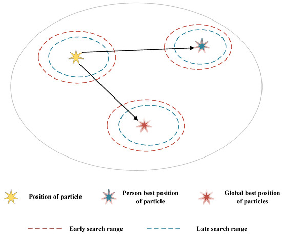
Figure 2. The schematic diagram for the search ranges in the early and late stages of OPSO. Source: own creation.

3.3. Framework of OPSO-LSTM Model

Enhancing the precision of carbon emission prediction models necessitates meticulous parameter optimization, specifically refining elements such as the number of neurons and the learning rate within the LSTM architecture. Nonetheless, the conventional approach of manual debugging proves arduous and time-intensive, prompting us to seek an innovative solution. We seamlessly integrate the OPSO algorithm into the LSTM framework, resulting in the OPSO-LSTM model. Within this framework, OPSO assumes the pivotal role of fine-tuning LSTM’s neuron count and learning rate, yielding significant enhancements in prediction accuracy.

The OPSO-LSTM model’s construction entails the orchestration of four fundamental components, each playing a crucial role in its overall efficacy. These components encompass data pre-processing, where raw data are refined and prepared for analysis; OPSO’s relentless pursuit of the optimal solution, model training, which involves iterative adjustments for optimal performance; and the eventual generation of predictions. To provide a visual aid in understanding this intricate process, we have included a detailed flowchart in Figure 3, shedding light on the sequence of operations. A comprehensive exploration of each of these components is shown as follows:

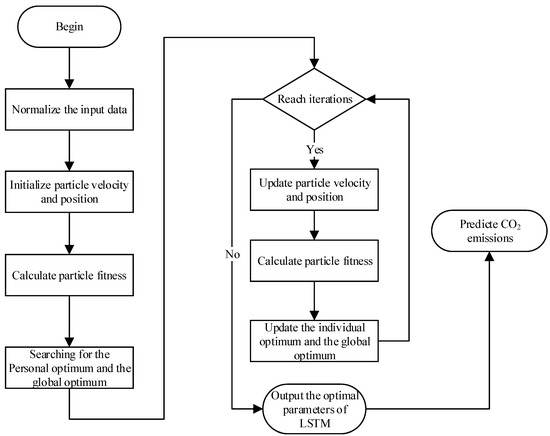
Figure 3. The flowchart of OPSO-LSTM. Source: own creation.

• Step 1: Normalize all the data within the range −1 to 1 according to the formula. The normalization formula is shown in Equation (9). The normalization can eliminate the influence of the scale between indicators to solve the comparability between data indicators.

  $$X_{norm}=2\ast (X-X_{min})/(X_{max}-X_{min})-1$$

  (9)

  where $X_{norm}$ is the output after normalization. $X_{min}$ and $X_{max}$ are the minimum and maximum values of the input class of data. X represents the input data.
• Step 2: In the OPSO optimization process, the number of neurons and initial learning rate of LSTM are taken as optimization objects, and the mean square error (MSE) is taken as a fitness function of OPSO. The fitness function of OPSO is as follows:

  $$Fitness=MSE=\frac{1}{n}\sum _{i=1}^n{(Y_i-\overline{Y_i})}^2$$

  (10)

  where n is the number of samples. $Y_i$ and $\overline{Y_i}$ are the true value and the predicted value, respectively.
• Step 3: The optimal number of neurons and the initial learning rate obtained by searching by OPSO are used as parameters during LSTM training.

4. Experiment and Results

To assess the performance of the OPSO-LSTM model, we conducted a series of simulation experiments utilizing authentic data. In these experiments, standard LSTM and PSO-LSTM are selected in the control group. Real data of carbon emission of Hainan Provenience are used in training and testing these models. Experimental details are presented in subsections.

4.1. Data Preparation

Understanding the intricate relationship between carbon dioxide (CO₂) emissions from energy consumption and a multitude of factors such as local gross domestic product (GDP), resident population, passenger and freight traffic, civilian vehicle ownership, and residential consumption levels is essential. To comprehensively explore this relationship, we have meticulously curated a comprehensive dataset spanning the years 1991 to 2021, specific to Hainan Province. This dataset encompasses a diverse array of ten crucial data categories, including GDP, retail sales of consumer goods (RSCG), production value of agriculture, forestry, animal husbandry, and fishery (PVAFAF), sown area of crops (SAC), value of building enterprises (VBE), resident population (RP), passenger traffic (PT), cargo volume (CV), civilian vehicle ownership (CVO), and resident consumption level (RCL). The detailed data tables, labeled as Table 1 and Table 2, contain the specific information. Our model training process utilized data from 1991 to 2016, while the subsequent evaluation of the OPSO-LSTM model’s reliability was conducted using data from the years 2017 to 2021. These data can be downloaded from the CEInet Statistics Database (https://db.cei.cn/jsps/Home) and Hainan Statistical Yearbook(HSY).

Table 1. The specific data of GDP, RSCG, PVAFAF, SAC, VBE, and RP (Source: CEInet Statistics Database and HSY).

Indicators	GDP	RSCG	PVAFAF	SAC	VBE	RP
Unit	Billion Yuan	Billion Yuan	Billion Yuan	Kha	Ten-Thousand Yuan	Ten-Thousand People
1991	120.52	41.97	78.78	829	153,000	674
1992	184.92	55.02	87.16	868	246,000	686
1993	260.41	72.91	120.25	884	507,000	701
1994	331.98	95.24	169.99	844	222,300	711
1995	363.25	110.09	202.52	870	175,900	723.79
1996	389.68	122.87	224.22	890.78	151,800	734.14
1997	411.16	135.2	234.86	914.51	279,900	743
1998	442.12	147.06	253.67	937.57	309,000	752.82
1999	476.68	160.62	279.23	931.76	333,933.3	761.93
2000	526.82	176.19	311.94	906	302,139	789
2001	579.18	192	325.13	871.73	353,452.6	795.55
2002	642.74	209.91	360.2	863.34	415,089	803.13
2003	713.96	197.33	379.98	906.74	394,053	810.52
2004	802.68	245.47	438.73	826.94	585,834	817.83
2005	884.87	281.58	475.88	778.06	596,925.2	828
2006	1027.45	326.77	492.12	699.4	649,436	835.88
2007	1234	387.78	547.03	757.71	821,834	845.03
2008	1474.66	485.68	662.07	793.61	1,111,836.9	854.18
2009	1620.28	573	700.23	800.44	1,439,441.5	864.07
2010	2020.53	698.81	813.8	786.75	1,994,842	868.55
2011	2463.84	866.92	991.53	782.4	2,554,721.8	889.61
2012	2789.38	1003.69	1067.33	786.57	2,831,087.1	910.43
2013	3115.85	1154.87	1125.93	772.48	2,863,073.3	920.21
2014	3449.01	1298.74	1227.14	779.4	2,763,288.9	935.56
2015	3734.19	1409.45	1294	757.5	2,786,307.6	945.49
2016	4090.2	1547.26	1433.88	731.9	3,077,647.7	957.48
2017	4497.54	1729.44	1488.86	709.44	3,227,630	971.5
2018	4910.69	1852.68	1535.73	712.94	3,576,139.8	982.48
2019	5330.84	1951.11	1689.4	676.24	3,659,800.3	995.27
2020	5566.24	1974.63	1821.02	676.86	3,913,714.1	1012.34
2021	6504.05	2497.62	2014.79	684.78	4,470,939.5	1020.46

Table 2. The specific data of PT, CV, CVO, RSL, and CO${}_2$ emissions from energy consumption (Source: CEInet Statistics Database and HSY).

Indicators	PT	CV	CVO	RSL	CO2 Emissions from Energy Consumption
Unit	Ten-Thousand People	Ten-Thousand Tons	Ten-Thousand Units	Yuan	Tons
1991	17,133	5710.55	3.66	833	536.61
1992	17,708	6252.78	4.92	1019	643.74
1993	19,010	8612.9	6.67	1363	725.25
1994	18,829	8735	8.63	1673	836.13
1995	19,667	10,505	9.52	1993	927.99
1996	19,688	10,975	9.87	2337	1056.24
1997	21,296	11,415.22	9.51	2432	1170.78
1998	21,549	11,629.67	9.06	2552	1227.78
1999	22,085	11,532.93	9.59	2729.26	1291.8
2000	23,013	11,304	9.01	2903.68	1439.85
2001	26,711	10,502.26	8.28	2961.37	1561.32
2002	27,992	10,497.94	10.94	3197.75	2051.22
2003	28,083	11,248.94	12.58	3275	2227.44
2004	31,276	11,823.48	14.55	3620	2466.6
2005	32,933	13,558.19	16.4	4145	2761.35
2006	36,326	16,377.08	19.23	4736	3171
2007	39,451	17,343.65	22.11	5552	3405.99
2008	44,186	16,847.04	25.81	6550	3697.56
2009	42,232	18,417.37	30.64	6695	4075.53
2010	45,718	22,481	39.24	7553	4801.86
2011	47,913	25,141	47.81	9237.66	5063.94
2012	49,015.38	26,906.4	55.46	10,634.49	5331.78
2013	51,000	28,833.5	64.8	11,712	5160.99
2014	16,775	23,081	75.11	12,915	5459.79
2015	16,284	22,330.2	83.29	17,019.13	5813.31
2016	17,092	21,828.2	96.32	18,431	6018.36
2017	18,154.57	21,397.22	113.21	20,939	6238.68
2018	18,314.17	22,093.2	126.9	22,971	6510.69
2019	18,104.85	18,552.39	137.24	19,555	6793.17
2020	9735	20,737	149.05	18,972	6811.92
2021	11,197	28,039	168.72	22,242	7338.57

4.2. OPSO-LSTM Forecasting Results

PSO and OPSO are used to optimize parameters of LSTM, indicate that OPSO is better than PSO in optimal LSTM, and verify the performance of the OPSO-LSTM in predicting the CO${}_2$ emissions from energy consumption of Hainan Province. We chose LSTM and POS-LSTM as the control group. To ensure fairness in the comparison, we used the same population size of 50 and number of iterations of 100 as PSO in our experiments, as well as the same range of optimized objects. The detailed parameters of the PSO and OPSO are shown in Table 3.

Table 3. The detailed parameters of the PSO and OPSO. Source: own creation.

Parameter	PSO	OPSO
Populations	50	50
Iterations	100	100
Range of learning rate	[0.001, 0.15]	[0.001, 0.15]
Range of neurons	[10, 50]	[10, 50]

We put the sample data into the control group and the proposed OPSO-LSTM for training and prediction. The curves of the control group and the proposed OPSO-LSTM training and prediction results are shown in Figure 4, Figure 5 and Figure 6. Data from 1991 to 2015 are used in training, and data from 2016 to 2021 are used in tests. With the accumulation of years of input data, the training results of OPSO-LSTM are basically consistent with the actual results and significantly better than PSO-LSTM and LSTM. In the prediction of the test, the OPSO-LSTM curves significantly fit the true values better. The specific results for the test data are shown in Table 4. Compared with the control group, the OPSO-LSTM model has the best prediction in 2017, 2019, and 2021. In the prediction of 2021, the error of OPSO-LSTM is only 1.29% lower than the 12.9% and 7.57% of LSTM and PSO-LSTM.

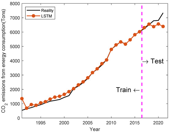
Figure 4. The training and prediction result of LSTM. Source: own creation.

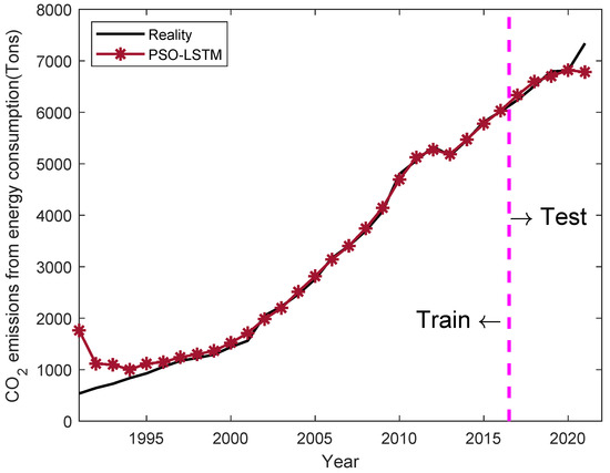
Figure 5. The training and prediction result of PSO-LSTM. Source: own creation.

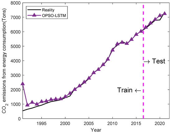
Figure 6. The training and prediction result of OPSO-LSTM. Source: own creation.

Table 4. The specific results for the test data. Source: own creation.

Year	Reality	LSTM		PSO-LSTM		OPSO-LSTM
		Prediction	Errors	Prediction	Errors	Prediction	Errors
2017	6238.68	6307.6	1.10%	6333.22	1.52%	6296.47	0.93%
2018	6510.69	6552.36	0.64%	6596.39	1.32%	6593.9	1.28%
2019	6793.17	6379.76	6.09%	6701.55	1.35%	6845.27	0.77%
2020	6811.92	6565.77	3.61%	6819.38	0.11%	7112.7	4.42%
2021	7338.57	6391.97	12.90%	6783.3	7.57%	7243.92	1.29%

To further demonstrate the advantages of OPSO-LSTM in predicting CO${}_2$ emissions from energy consumption in Hainan Province, we chose the three most common forecast evaluation metrics, including mean absolute error (MAE), root mean square error (RMSE), and mean absolute percentage error (MAPE), to calculate specific data for LSTM, PSO-LSTM, and OPSO-LSTM on the test set. The MEA is used to calculate the mean error between the true and predicted values. The RMSE is a metric that presents the fitting effect metric. Compared to the MAE, the MAPE normalizes the error between the true and predicted values for each pair, decreasing the contribution of absolute errors for individual outliers. The detailed calculations of these indicators are shown in Table 5, and the equations of the MAE, RMSE, and MAPE are as follows:

$$MAE=\frac{1}{n}\sum _{i=1}^n|P_i-R_i|$$

(11)

$$RMSE=\sqrt{\frac{1}{n}\sum _{i=1}^n{(P_i-R_i)}^2}$$

(12)

$$MAPE=\frac{1}{n}\sum _{i=1}^n|\frac{P_i-R_i}{R_i}|$$

(13)

where n is the number of samples. $P_i$ and $R_i$ are the prediction value and reality value, respectively.

Table 5. The LSTM, PSO-LSTM and OPSO-LSTM with specific MEA, RMSE and MAPE on the test set. Source: own creation.

Indicators	LSTM	PSO-LSTM	OPSO-LSTM
MAE	343.349	166.917	117.708
Difference with OPSO-LSTM	65.72%	29.48%
RMSE	476.243	258.090	149.939
Difference OPSO-LSTM	68.52%	41.90%
MAPE	0.049	0.024	0.017
Difference OPSO-LSTM	65.31%	29.17%

Compared with the LSTM and PSO-LSTM models, the MAE of OPSO-LSTM is 117.708, 65.72% better than LSTM and 29.48% better than PSO-LSTM. The RMSE of OPSO-LSTM is 149.939, 68.52% better than LSTM and 41.90% better than PSO-LSTM. The MAPE of OPSO-LSTM is 0.017, 65.31% better than LSTM and 29.17% better than PSO-LSTM. All the indicators indicate that the OPSO-LSTM is superior to the LSTM and PSO-LSTM. However, it is worth noticing that in the years 2020 and 2021, there is a significant change in the prediction accuracy of all methods. This is caused by the dramatic changes in the economy caused by COVID-19. Therefore, improving model stability against drastic economic changes is a valuable future work.

5. Conclusions

In this paper, a novel OPSO-LSTM model for carbon emissions prediction is proposed. OPSO-LSTM combines two key components: OPSO (oscillatory particle swarm optimization) and LSTM (long short-term memory). OPSO is employed to fine-tune the hyperparameters of the LSTM, utilizing an oscillatory strategy to effectively mitigate overfitting and consequently improve the accuracy of the LSTM model. To verify the predictive ability of the proposed model, simulation experiments are implemented. The standard LSTM and PSO-LSTM are selected in the control group. Real data from Hainan Province, encompassing diverse dimensions such as gross domestic product, forest area, and ten other relevant factors, are used in model training and testing. The mean absolute error (MAE), root mean square error (RMSE), and mean absolute percentage error (MAPE) are used to evaluate the performance of these methods. In the test dataset, the MAE of OPSO-LSTM is 117.708, 65.72% better than LSTM and 29.48% better than PSO-LSTM. The RMSE of OPSO-LSTM is 149.939, 68.52% better than LSTM and 41.90% better than PSO-LSTM. The MAPE of OPSO-LSTM is 0.017, 65.31% better than LSTM and 29.17% better than PSO-LSTM. Compared with the LSTM model and the PSO-LSTM model, OPSO-LSTM is able to overcome the model instability problem caused by the difficulty of hyperparameter selection. The experimental results show that OPSO-LSTM is able to provide high-precision results for carbon emission prediction tasks.

The OPSO-LSTM model empowers industries, policymakers, and environmentalists with the capability to make data-driven decisions, optimize energy consumption, allocate resources efficiently, and advance sustainable practices, thereby playing a pivotal role in addressing climate change and environmental impact assessment and shaping a more sustainable future.

Considering the ongoing technological advancements in neural networks, we believe that exploring the impact of high-dimensional input data on OPSO’s prediction accuracy is a crucial future endeavor. Additionally, choosing a more suitable adaptive function for optimizing LSTM parameters can significantly affect model accuracy. Furthermore, improving the training speed of OPSO-LSTM for real-time predictions is an achievable future goal.

References

- Abeydeera, L.H.U.W.; Mesthrige, J.W.; Samarasinghalage, T.I. Global research on carbon emissions: A scientometric review. Sustainability 2019, 11, 3972. [Google Scholar] [CrossRef]
- Wang, X.; Chen, H.; Gan, C.; Lin, H.; Dou, Q.; Tsougenis, E.; Huang, Q.; Cai, M.; Heng, P.A. Weakly Supervised Deep Learning for Whole Slide Lung Cancer Image Analysis. IEEE Trans. Cybern. 2020, 50, 3950–3962. [Google Scholar] [CrossRef] [PubMed]
- Jin, H. Prediction of direct carbon emissions of Chinese provinces using artificial neural networks. PLoS ONE 2021, 16, e0236685. [Google Scholar] [CrossRef]
- Gao, P.; Yue, S.; Chen, H. Carbon emission efficiency of China’s industry sectors: From the perspective of embodied carbon emissions. J. Clean. Prod. 2021, 283, 124655. [Google Scholar] [CrossRef]
- Cai, H.; Wang, Z.; Zhu, Y. Understanding the structure and determinants of intercity carbon emissions association network in China. J. Clean. Prod. 2022, 352, 131535. [Google Scholar] [CrossRef]
- Kılıç, M.; Kuzey, C. The effect of corporate governance on carbon emission disclosures: Evidence from Turkey. Int. J. Clim. Chang. Strateg. Manag. 2019, 11, 35–53. [Google Scholar] [CrossRef]
- Waheed, R.; Sarwar, S.; Wei, C. The survey of economic growth, energy consumption and carbon emission. Energy Rep. 2019, 5, 1103–1115. [Google Scholar] [CrossRef]
- Lee, J.H.; Cho, J.H. Firm-value effects of carbon emissions and carbon disclosures—Evidence from korea. Int. J. Environ. Res. Public Health 2021, 18, 12166. [Google Scholar] [CrossRef]
- Alam, M.S.; Safiullah, M.; Islam, M.S. Cash-rich firms and carbon emissions. Int. Rev. Financ. Anal. 2022, 81, 102106. [Google Scholar] [CrossRef]
- Bai, J.; Chen, Z.; Yan, X.; Zhang, Y. Research on the impact of green finance on carbon emissions: Evidence from China. Econ. Res.-Ekon. Istraz. 2022, 35, 6965–6984. [Google Scholar] [CrossRef]
- Ott, C.; Schiemann, F. The market value of decomposed carbon emissions. J. Bus. Financ. Account. 2023, 50, 3–30. [Google Scholar] [CrossRef]
- Chen, X.; Cheng, F.; Liu, C.; Cheng, L.; Mao, Y. An improved Wolf pack algorithm for optimization problems: Design and evaluation. PLoS ONE 2021, 16, e0254239. [Google Scholar] [CrossRef] [PubMed]
- Mou, X.; Zhang, Y.; Jiang, J.; Sun, H. Achieving Low Carbon Emission for Dynamically Charging Electric Vehicles through Renewable Energy Integration. IEEE Access 2019, 7, 118876–118888. [Google Scholar] [CrossRef]
- Ahvar, E.; Ahvar, S.; Mann, Z.A.; Crespi, N.; Glitho, R.; Garcia-Alfaro, J. DECA: A Dynamic Energy Cost and Carbon Emission-Efficient Application Placement Method for Edge Clouds. IEEE Access 2021, 9, 70192–70213. [Google Scholar] [CrossRef]
- Zhou, F.; Huang, Z.; Zhang, C. Carbon price forecasting based on CEEMDAN and LSTM. Appl. Energy 2022, 311, 118601. [Google Scholar] [CrossRef]
- Kong, F.; Song, J.; Yang, Z. A novel short-term carbon emission prediction model based on secondary decomposition method and long short-term memory network. Environ. Sci. Pollut. Res. 2022, 29, 64983–64998. [Google Scholar] [CrossRef]
- Hu, Y.; Lv, K. Hybrid prediction model for the interindustry carbon emissions transfer network based on the grey model and general vector machine. IEEE Access 2020, 8, 20616–20627. [Google Scholar] [CrossRef]
- Wang, J.; Xie, Y.; Xie, S.; Chen, X. Cooperative particle swarm optimizer with depth first search strategy for global optimization of multimodal functions. Appli. Intell. 2022, 52, 10161–10180. [Google Scholar] [CrossRef]
- Gao, M.; Yang, H.; Xiao, Q.; Goh, M. A novel fractional grey Riccati model for carbon emission prediction. J. Clean. Prod. 2021, 282, 124471. [Google Scholar] [CrossRef]
- Wang, T.; Li, Z.; Geng, X.; Jin, B.; Xu, L. Time Series Prediction of Sea Surface Temperature Based on an Adaptive Graph Learning Neural Model. Future Internet 2022, 14, 171. [Google Scholar] [CrossRef]
- Cai, J.; Ma, X. Carbon emission prediction model of agroforestry ecosystem based on support vector regression machine. Appl. Ecol. Environ. Res. 2019, 17, 6397–6413. [Google Scholar] [CrossRef]
- Kong, F.; Song, J.; Yang, Z. A daily carbon emission prediction model combining two-stage feature selection and optimized extreme learning machine. Environ. Sci. Pollut. Res. 2022, 29, 87983–87997. [Google Scholar] [CrossRef] [PubMed]
- Huang, W.; Dong, S. Improved short-term prediction of significant wave height by decomposing deterministic and stochastic components. Renew. Energy 2021, 177, 743–758. [Google Scholar] [CrossRef]
- Zhao, S.; Patuano, A. International chinese students in the uk: Association between use of green spaces and lower stress levels. Sustainability 2022, 14, 89. [Google Scholar] [CrossRef]
- Lu, X.; Ota, K.; Dong, M.; Yu, C.; Jin, H. Predicting Transportation Carbon Emission with Urban Big Data. IEEE Trans. Sustain. Comput. 2017, 2, 333–344. [Google Scholar] [CrossRef]
- Greff, K.; Srivastava, R.K.; Koutnik, J.; Steunebrink, B.R.; Schmidhuber, J. LSTM: A Search Space Odyssey. IEEE Trans. Neural Netw. Learn. Syst. 2017, 28, 2222–2232. [Google Scholar] [CrossRef] [PubMed]
- Abbasimehr, H.; Shabani, M.; Yousefi, M. An optimized model using LSTM network for demand forecasting. Comput. Ind. Eng. 2020, 143, 106435. [Google Scholar] [CrossRef]
- Zhao, J.; Kou, L.; Wang, H.; He, X.; Xiong, Z.; Liu, C.; Cui, H. Carbon Emission Prediction Model and Analysis in the Yellow River Basin Based on a Machine Learning Method. Sustainability 2022, 14, 6153. [Google Scholar] [CrossRef]
- Guo, J.; Sato, Y. A Pair-wise Bare Bones Particle Swarm Optimization Algorithm for Nonlinear Functions. Int. J. Netw. Distrib. Comput. 2017, 5, 143. [Google Scholar] [CrossRef]
- Tian, H.; Guo, J.; Xiao, H.; Yan, K.; Sato, Y. An electronic transition-based bare bones particle swarm optimization algorithm for high dimensional optimization problems. PLoS ONE 2022, 17, e0271925. [Google Scholar] [CrossRef]
- Guo, X.; He, J.; Wang, B.; Wu, J. Prediction of Sea Surface Temperature by Combining Interdimensional and Self-Attention with Neural Networks. Remote Sens. 2022, 14, 4737. [Google Scholar] [CrossRef]
- Guo, J.; Zhou, G.; Yan, K.; Shi, B.; Di, Y.; Sato, Y. A novel hermit crab optimization algorithm. Sci. Rep. 2023, 13, 9934. [Google Scholar] [CrossRef] [PubMed]
- Xiao, H.; Guo, J.; Shi, B.; Di, Y.; Pan, C.; Yan, K.; Sato, Y. A Twinning Memory Bare-bones Particle Swarm Optimization Algorithm for No-linear Functions. IEEE Access 2022, 11, 25768–25785. [Google Scholar] [CrossRef]
- Li, J.; Tian, Z.; Zhang, G.; Li, W. Multi-AUV Formation Predictive Control Based on CNN-LSTM under Communication Constraints. J. Mar. Sci. Eng. 2023, 11, 873. [Google Scholar] [CrossRef]
- Guo, J.; Sato, Y. A fission-fusion hybrid bare bones particle swarm optimization algorithm for single-objective optimization problems. Appl. Intell. 2019, 49, 3641–3651. [Google Scholar] [CrossRef]
Disclaimer/Publisher’s Note: The statements, opinions and data contained in all publications are solely those of the individual author(s) and contributor(s) and not of MDPI and/or the editor(s). MDPI and/or the editor(s) disclaim responsibility for any injury to people or property resulting from any ideas, methods, instructions or products referred to in the content. |
© 2023 by the authors. Licensee MDPI, Basel, Switzerland. This article is an open access article distributed under the terms and conditions of the Creative Commons Attribution (CC BY) license (https://creativecommons.org/licenses/by/4.0/).