Application of the Heat Penetration Distance in the Design of the Hole Spacing of Ground-Coupled Heat Pumps

Abstract

Due to issues such as heat accumulation, the site area, and project investment, the reasonable determination of the hole spacing for heat exchangers has become one of the key design points of the ground-coupled heat pump system. Based on the definition of heat penetration in heat transfer and the research method of the inverse problem, a direct algorithm of the heat penetration distance in the aquifer was proposed using the analytical solution to the mathematical model for one-dimensional heat convection–conduction problems. Taking a vertical ground-coupled heat pump project in Hefei, Anhui Province, China, as an example, a three-dimensional hydro-thermal coupling numerical simulation model was established, and the influence radius during the refrigeration and heating periods under the action of a single borehole heat exchanger was determined. Comparing the heat penetration distance with the influence radius, the results show that the relative errors of the results obtained by the two methods are less than 10%, which verifies the rationality and effectiveness of the calculated penetration distance in the aquifer. At the end of the cooling or heating period, the heat penetration distance in the aquifer is calculated to be 7.59 m. Therefore, the proposed method is straightforward and efficient, which can provide a convenient approach to determining the reasonable hole spacing of the heat pump system.

1. Introduction

Shallow geothermal energy (SGE), as a new clean and environmentally friendly energy source, has been strongly promoted in China, the European Union, and other places due to its wide distribution, stable temperature, and convenient collection [1]. In the development and utilization of SGE, the most widely used technology is the ground-coupled heat pump (GCHP), that is, a heat pump system that employs low-grade thermal energy stored in the ground to achieve the cooling and heating of buildings through heat exchangers [2].

In the practical application of GCHP technology, problems such as thermal interference and thermal accumulation are prone to occur, which seriously affect the sustainable development and utilization of SGE [3]. Among them, the irrational hole spacing design of ground heat exchangers (GHEs) is one of the key factors leading to such problems. If the hole spacing is too small, it will cause thermal interference between adjacent GHEs and reduce the heat transfer efficiency between the GHE and the ground, which will affect the performance of the GCHP system; if the hole spacing is too large, it will require a larger area of the site and a higher initial investment [3,4]. Therefore, the reasonable arrangement of GHEs within the limited site area is an important factor in the design of GCHP systems. Most of the existing literature quantifies the effect of hole spacing on soil temperature by site test investigation or establishing a numerical simulation model or a simulation platform, based on which the appropriate hole spacing is determined. The experimental investigation conducted by Yu et al. shows that the heat transition capability of soil improves with an increased hole spacing, and the borehole spacing is recommended as 4–5 m in Shanghai [5]. Du et al. established a 3D thermo-hydraulic coupled numerical model, and the simulation results indicate that the heat accumulation phenomenon will disappear with the hole spacing of heat exchangers increasing from 5 m to 14, 17, 18, 21, and 19 m [3]. Zhang et al. built a 3D finite-element dynamic simulation platform considering the impact of freezing and groundwater seepage to analyze the performance of a GCHP system [4]. According to the study, increasing the hole spacing can drastically shorten the soil’s freezing penetration distance. When the borehole spacing is 4.5 m or 5.5 m as opposed to 3.5 m, its maximum freezing penetration distance decreases by 0.23 m and 0.41 m in the unsaturated area and by 0.19 m and 0.33 m in the saturated area, respectively. Zhang et al. established a simulation model using TRNSYS and studied the influence extent of various factors on the soil thermal balance by an orthogonal experimental design method [6]. The research reveals that the proposed maximum comprehensive coefficient of performance of the whole-year transportation system decreases with the increase in hole spacing, and the reasonable spacing of the system should be 4–5 m. However, either the experimental investigation or the establishment, identification, and validation of a reasonable numerical model or platform require a mass of fundamental data, so the data collection and model adjustment are laborious and time-consuming.

Whether the thermal breakthrough occurs in the soil under the continuous effect of the GCHP system is an important indicator of whether the ground can provide a steady heat exchange for a long time and is also the basis for the long-term stable operation of the heat pump system. The thermal breakthrough process in soil and the heat penetration in heat transfer studies have the same mathematical and physical significance. Therefore, referring to the research methodology of the inverse problem, the heat penetration distance in the aquifer is calculated based on the analytical solution to the mathematical model for one-dimensional heat convection–conduction problems. Subsequently, the influence radius of a vertical GCHP project in Hefei is determined by numerical simulation under the action of a single borehole heat exchanger (BHE) and compared with the heat penetration distance calculation results presented in the paper to verify the reasonableness of the obtained heat penetration distance. The proposed calculation method is straightforward and convenient, which can provide strong technical support for the reasonable determination of hole spacing for GHEs in the design stage of GCHP systems.

2. Heat Penetration Distance

2.1. Definition

In the semi-infinite domain, for the one-dimensional heat conduction issue bounded by Dirichlet conditions, the boundary temperature in the classical model is constant after an instantaneous change in ∆T₀ from the initial temperature, and then the excess temperature at the distance x from the boundary [7] can be expressed as

$$T\left(x,t\right)=\Delta T_0·\mathrm{erfc}\left(\frac{x}{2\sqrt{at}}\right)$$

(1)

where T(x,t) is the function of excess temperature at moment t and at distance x from the boundary (°C), x is the distance from the border (m), t denotes the time (d), ∆T₀ is the temperature variation at the boundary (°C), and a is the thermal diffusivity (m²/d).

Let µ = x/2$\sqrt{at}$ when erf(µ) = 0.9953, i.e., erfc(µ) = 1 − erf(µ) = 0.0047 [8]; then, we have T(x,t)/∆T₀ < 5‰, and at this moment, µ = 2. Hereby, the time corresponding to µ = 2 is defined as the inert time τ, and the corresponding x is denoted as x_max(τ), which is defined as the heat penetration distance. The heat penetration distance is a physical quantity that indicates the distance of heat diffusion in the materials [9,10], and in this study, we define it as the maximum distance within time t formed by the continuous action of the Dirichlet boundary [8], that is, the boundary heat source has essentially no effect on the region larger than the “heat penetration distance” within time t.

2.2. The Calculation Method of the Heat Penetration Distance in the Aquifer

The effect of groundwater cannot be neglected for the heat transfer problem of the GCHP system in the aquifer. Therefore, the heat transfer not only includes the heat conduction of the solid skeleton constituting the aquifer but also involves the heat convection formed by the groundwater transport, i.e., the heat transfer process of the GCHP system in the aquifer is dominated by the superposition equation of the thermal convection effect of groundwater migration and the heat conduction process of the medium in the water-bearing layer. In a homogeneous, isotropic, and infinitely spreading horizontal aquifer, assuming that the heat transfer between the groundwater and the solid skeleton is instantaneous, the heat transport in the aquifer can be regarded as a one-dimensional convection-diffusion process in the horizontal direction [11], i.e., the heat transfer mechanism in the water-bearing layer caused by the action of the GCHP system is essentially a one-dimensional heat convection–conduction problem bound by Dirichlet conditions in a half-space.

The basic differential equation of the heat convection–conduction model is the viscous Burgers’ equation, which has been rarely studied analytically due to the difficulty in solving the analytical solution. Therefore, the analytical solution of a similar mathematical model whose basic differential equation is also the viscous Burgers’ equation, i.e., the solute transport model in the aquifer, can be referred to.

The one-dimensional convection–dispersion model of contaminant transport in a homogeneous aquifer under the condition that the concentration at the origin changes instantaneously by ∆c₀ and subsequently remains constant can be described by the mathematic model (Ⅰ) that follows [12,13]:

$$\{\begin{array}{c}\frac{\partial c\left(z,t\right)}{\partial t}=D_z\frac{{\partial }^{2}c}{\partial z^2}\begin{array}{cc}-v_z\frac{\partial \mathrm{c}}{\partial z}& 0<z<+\infty ,t>0\end{array}\\ {c\left(z,t\right)|}_{t=0}=0 x>0\\ {c\left(z,t\right)|}_{z=0}=\Delta c_0 t>0\\ {c\left(z,t\right)|}_{z\to \infty }=0 t>0\end{array}$$

(2)

where z is the vertical transport distance (m), c(z,t) is the pollutant concentration at a vertical distance z from the boundary at moment t (mg/L), ∆c₀ is the continuous point source concentration of contaminants under the Dirichlet boundary condition (mg/L), D_z is the vertical dispersion coefficient (m²/d), and v_z is the vertical seepage velocity (m/d).

The analytical solution to the model (Ⅰ) can be given through the Laplace transformation as [12]:

$$c\left(x,t\right)=\frac{\Delta c_0}{2}\mathrm{erfc}\left(\frac{z-v_{z}t}{2\sqrt{D_{z}t}}\right)+\frac{\Delta c_0}{2}\exp (\frac{v_{z}z}{D_z})\cdot \mathrm{erfc}\left(\frac{z+v_{z}t}{2\sqrt{D_{z}t}}\right)$$

(3)

Referring to Equation (3), we obtain:

$$T\left(x,t\right)=\frac{\Delta T_0}{2}\mathrm{erfc}\left(\frac{x-vt}{2\sqrt{at}}\right)+\frac{\Delta T_0}{2}\exp (\frac{vx}{a})\cdot \mathrm{erfc}\left(\frac{x+vt}{2\sqrt{at}}\right)$$

(4)

where v indicates the groundwater velocity in the aquifer (m/d).

From Equation (4), the second term at the right end has a certain effect only under the condition that x→0; so as long as the calculation point is at a certain distance from the boundary, the second term at the right end is negligible because it is much smaller than the first term at the right end [12]; then, Equation (4) can be abbreviated as:

$$T\left(x,t\right)=\frac{\Delta T_0}{2}\Delta \mathrm{erfc}\left(\frac{x-vt}{2\sqrt{at}}\right)$$

(5)

Comparing Equations (1) and (5), the physical meanings expressed by the equations are different, but the mathematical models are identical, i.e., there should be consistency in the mathematical physical laws reflected by the equations.

From the above definition of the heat penetration distance, µ = 2, we have:

$$x_{\max }\left(\tau \right)=4\sqrt{a\tau }+v\tau$$

(6)

where τ is defined as the inertia time in the study of heat transfer problems (d), and x_max(τ) is the heat penetration distance corresponding to time τ (m).

Equation (6) is the proposed equation for calculating the heat penetration distance by the analytical method.

3. Materials and Methods

To verify the reasonableness of the above calculation method of the heat penetration distance, a vertical GCHP system project in Hefei (the location of the project is shown in Figure 1) is taken as an example, and a three-dimensional hydro-thermal coupling numerical simulation is carried out.

3.1. Geological Survey

Hefei City is located in the central part of Anhui Province and has a humid subtropical monsoon climate. The topography of the main urban area slopes from northwest to southeast, with three types of landforms in the area: hilly lands, low mountain residual hills, and low-lying plains. The strata in most areas of Hefei are Mesozoic strata, and the upper part of the strata in the city area is widely covered by the loose sediments of the Quaternary. The underlying strata of the Quaternary loose layer mainly include the early Cretaceous Zhuxiang Formation (K₁z), the late Cretaceous Zhangqiao Formation (K₂z), the Eocene Dingyuan Formation of Eogene (E₁dn), the Quaternary Holocene (Q₄), the Quaternary Pleistocene (Q₃), and the late Jurassic Zhougongshan Formation (J₃z). Groundwater is mainly stored in the loose layer of the Quaternary, with a thickness of about 20–50 m and an average groundwater velocity of 0.003 m/d. The loose layer is a confined aquifer, the upper part of which consists of sandy gravel, and the middle and lower parts are composed of middle-fine sandstone, fine sandstone, and sandy conglomerate. The overlying stratum of the loose layer is mainly composed of variegated mild clay endowed with fissure phreatic water, and the underlying stratum mainly consists of siltstone, silty mudstone, and muddy siltstone endowed with fissure-pore water.

According to the test results of several boreholes, the constant temperature zone in Hefei is below the ground’s depth of 20 m, and the floating range of ground temperature is 18–21 ℃.

3.2. Numerical Method

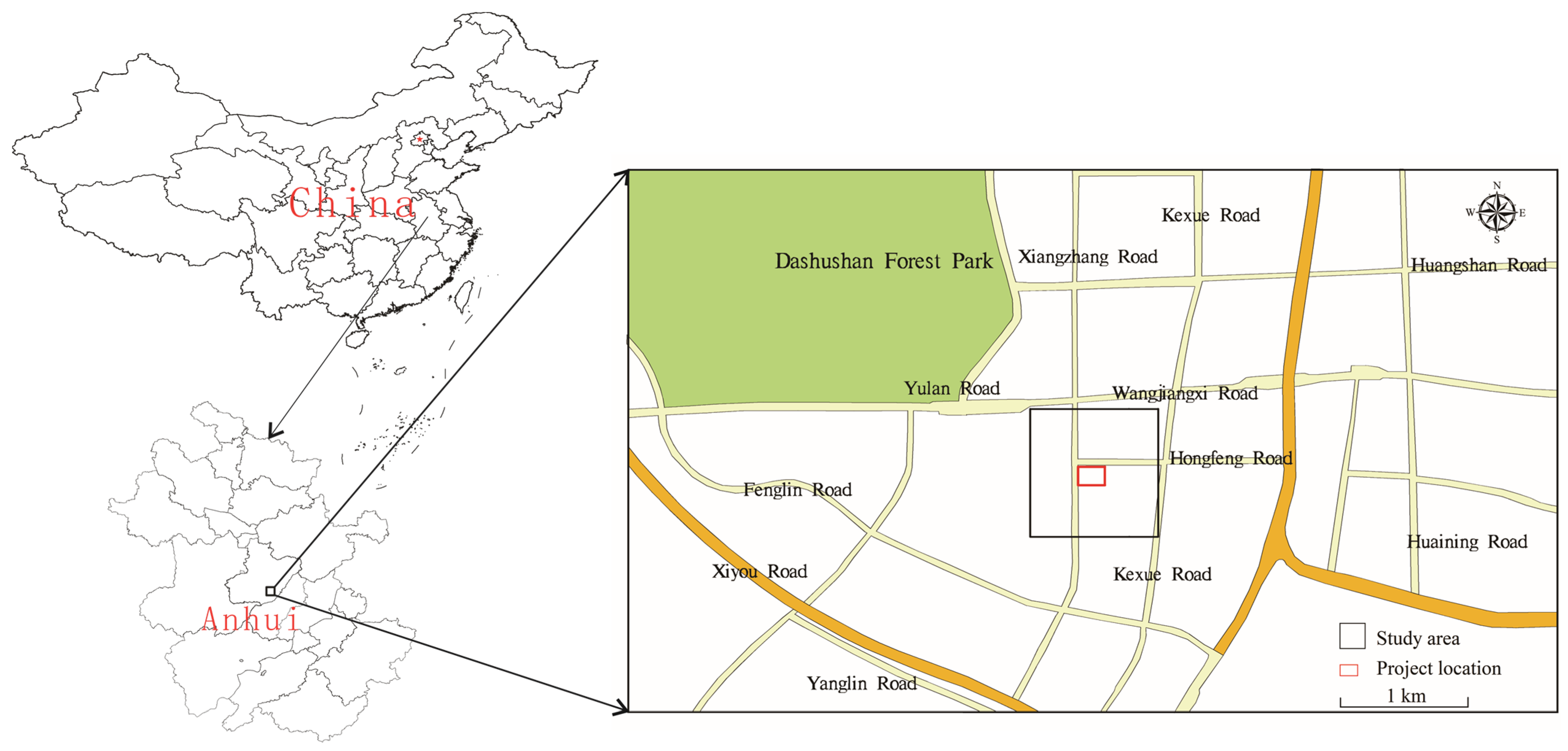
3.2.1. Study Area

The scope of the simulation area is determined mainly based on the hydrogeological conditions, stratigraphic characteristics, groundwater flow field, and pumping tests of the section where the example is located. Horizontally, a square area of 1 km × 1 km with the midpoint of the group of BHEs as the geometric center is taken as the study area; vertically, it is generalized into seven layers from top to bottom (see

Table 1. Stratification table of the strata in the study area.

Layer Number	Geological Time	Thickness	Lithological Description	Features
1	Q4	20	grayish yellow, reddish-brown clay, and mild clay	impermeable layer
2	Q3	2	grayish yellow mild clay
3	Q2	4	brown-yellow clay and mild clay
4	E1dn	1.5	gravel	aquifer
5		2.5	brown and tawny moderately weathered muddy siltstone
6		20	brown and tawny strongly weathered muddy siltstone
7	E1dn	150	brown, tawny, muddy siltstone and middle-fine sandstone	impermeable layer

), and the surface between adjacent strata, the top surface of the top plate, and the bottom surface of the bottom plate are all slices, assuming that each layer is homogeneous and isotropic. The aquifer is distributed in four to six layers with a burial depth of 26–50 m, in which the BHEs penetrate two to seven layers.

3.2.2. Mathematic Model

The mass and thermal energy of the water flow in the aquifer are in accordance with the law of the conservation of mass and energy, which can be expressed by the following mathematical equation [14]:

$$\{\begin{array}{c}{s}_{\mathrm{s}}\frac{\partial h}{\partial t}+\nabla ·\mathit{q}=Q+\gamma \left(\mathit{q}·\nabla T_s+n\frac{\partial T_s}{\partial t}\right)\\ \frac{\partial }{\partial t}\left\{\left[n{\rho }_w{c}_w+\left(1-n\right){\rho }_s{c}_s\right]T_s\right\}+\nabla ·\left({\rho }_w{c}_w\mathit{q}{T}_s\right)-\nabla ·\left(\Lambda ·\nabla T_s\right)=H_s\end{array}$$

(7)

where s_s is the storage coefficient of the solid skeleton in the aquifer, h is the hydraulic head of the aquifer (m), t represents time (s), ∇ is the vector differential operator, q is the Darcy velocity vector (m/s), Q is the flow rate (m³/s), γ is the thermal expansion coefficient of water (°C⁻¹), T_s is the temperature of the solid skeleton (°C), n is the porosity, c_w and c_s are the specific heat capacities of the water and the solid skeleton at the reference hydraulic head and reference temperature, respectively (J/(kg∙°C)), ρ_w and ρ_s are the densities of the water and the solid skeleton, respectively (kg/m³), Λ is the thermal diffusion tensor, and H_s is the source-sink term of heat (W/m).

According to Darcy’s law, q in porous media can be expressed as

$$\mathit{q}=-\mathit{K}{f}_{\mu }\Delta \left(\nabla h+\frac{{\rho }_w+{\rho }_{w0}}{{\rho }_{w0}}\mathit{e}\right)$$

(8)

where K is the tensor of hydraulic conductivity (m/s), f_μ is the constitutive viscosity relation function, ρ_w0 is the reference fluid density (kg/m³), and e is the gravitational unit vector.

For Λ, we have [15,16]

$$\Lambda =\left[n{\lambda }_w+\left(1-n\right){\lambda }_s\right]\mathit{I}+{\rho }_w{c}_w\left[{\alpha }_T\Vert \mathit{q}\Vert \mathit{I}+\left({\alpha }_L-{\alpha }_T\right)\frac{q\otimes q}{\Vert q\Vert }\right]$$

(9)

where λ_w and λ_s represent the thermal conductivity of the water and the solid skeleton, respectively (W/(m∙°C)), I is the unit tensor, and α_L and α_T are the longitudinal and transverse thermal dispersions, respectively (m).

For the seepage field, the initial boundary conditions are as follows:

$$\{\begin{array}{c}H\left(x,y,z,t\right)|{}_{t=0}=H_0\left(x,y,z,t\right) \left(x,y,z\right)ϵ\Omega , t\ge 0 \\ H\left(x,y,z,t\right)|{}_{\Gamma =0}=H_1\left(x,y,z,t\right) \left(x,y,z\right)ϵ{\Gamma }_1,t\ge 0\end{array}$$

(10)

where H₀ is the initial hydraulic head function of the aquifer, H₁ is the given hydraulic head function at the boundary of Γ, and Γ is the hydraulic head boundary of the aquifer.

For the temperature field, there are initial boundary conditions

$$\{\begin{array}{c}T\left(x,y,z,t\right)|{}_{t=0}=T_0\left(x,y,z,t\right) \left(x,y,z\right)ϵ\Omega , t\ge 0\\ T\left(x,y,z,t\right)|{}_{{\Gamma }_1=0}=T_1\left(x,y,z,t\right) \left(x,y,z\right)ϵ{\Gamma }_1,t\ge 0\end{array}$$

(11)

where T₁ is the temperature distribution function for the first type of temperature boundary conditions, and Γ₁ is the first type of temperature boundary. It should be noted that the detailed values of the boundary conditions of this GCHP project are shown in Section 3.2.5.

Coupling Equation (7) with Equations (10) and (11) constitutes a complete three-dimensional hydraulic–thermal coupled mathematical model of the aquifer in the study area.

3.2.3. Simulation Software Selection

This simulation uses the finite-element program FEFLOW [17], which resolves the equations regulating the flow, mass, and heat transfer in saturated or variable saturated systems using the standard iterative method [18].

3.2.4. Mesh Generation

The spatial discretization in this simulation is carried out using the triangle grid generation method, which employs the continuous Galerkin finite-element technique as its foundation [19].

Horizontally, each layer of the study area is separated into 11,007 elements and 5546 nodes, in which the group of BHEs (consisting of 20 heat exchangers, with a hole spacing of 8 m) is locally grid-encrypted. Vertically, the study area is divided into 77,049 elements and 44,368 nodes based on the lithology and thickness of the above-mentioned strata with an unequal interval division (see Figure 2).

3.2.5. Model Settings

The aquifer seepage field is considered a steady state, while the aquifer temperature field is considered an unsteady state due to the convective effect of the water flow for the heat transport and the operation of the GCHP system.

Since the direction of the groundwater flow is nearly an east–west orientation, the boundary conditions are set by generalizing the east and west sides of the study area to the given hydraulic head boundaries, and the north and south sides are set to the zero-flow-rate boundaries. The average surface elevation of the study area is 35 m, combined with the actual geohydrologic conditions; the hydraulic head on the west side is assigned to 12 m, and that on the east side is 8 m. The natural hydraulic slope is 0.4%, and the groundwater flow is steady flow from west to east.

The top plate of the stratum in the study area is a natural geothermal boundary, where the surface temperature is affected by solar radiation. To describe this daily variation process of geothermal temperature, the constant temperature boundary is set, and then the daily time series of geothermal temperature variation is established and superimposed on the constant temperature boundary as a modulation function.

The bottom plate of the stratum is affected by the geothermal heat flow and is set as the heat flux boundary. The average geothermal heat flow in Anhui Province is 62.0 mW/m² [20], so the heat flux is assigned as −0.062 W/m², and the maximum temperature constraint is set as 25 °C. The initial ground temperature of every other layer is assigned based on the measurement results of the temperature sensors buried in the observation hole before the operation of the GCHP system, combined with the interpolated extrapolation.

Combined with the actual project, both the cooling and heating periods of the system are 90 days. The inlet water temperature of BHEs during the cooling period is set to 36.4 °C, and that of the heating period is 7 °C.

3.2.6. Model Parameters

The initial and boundary water level and temperature values are substituted into the model, and for the model aquifer parameters, the initial values can be obtained based on data from pumping tests and thermal parameters tests firstly. In particular, under the condition that the data cannot meet the requirements of the numerical model, the analytical method can be used to calculate the relevant parameter values [21].

Subsequently, the initial values of the parameters are input into the model for trial runs, based on which continuous parameter inversion adjustments are performed, and the model is identified using the measured values of the water level from the pumping test and the temperature measurements from the ground temperature recovery test under the operation of a single BHE.

Finally, the model is validated by the ground temperature recovery test under the conditions of the simultaneous operation of 20 BHEs, and the hydrogeological and thermal properties of each layer are obtained (see

Table 2. Statistics of stratigraphic parameters in the study area.

Layer	Hydrogeologic Parameters					Thermal Properties of Solid
	Conductivity			Porosity	Specific Storage	Volumetric Heat Capacity	Thermal Conductivity
	Kx/m·d−1	Ky/m·d−1	Kz/m·d−1	n	μ *	cs/J·(kg·°C)−1	λs/w·(m·°C)−1
1	0.002	0.002	0.0002	0.3	0.0001	1.4 × 103	1.5
2	0.005	0.005	0.0005	0.3	0.0002	1.0 × 103	1.8
3	0.001	0.001	0.0001	0.25	0.0001	1.4 × 103	1.5
4	1.5	1.5	0.15	0.3	0.001	1.1 × 103	2.0
5	1.5	1.5	0.15	0.4	0.001	1.2 × 103	1.9
6	1.5	1.5	0.15	0.3	0.001	1.2 × 103	1.9
7	0.01	0.01	0.001	0.3	0.00001	1.2 × 103	1.8

).

4. Results

Taking the aquifer buried at a depth of 50 m (layer 6–slice 7) in the study area as an example, the calculation of the heat penetration distance in the aquifer under the action of a single BHE is carried out based on Equation (6) and compared with the numerical simulation results.

4.1. Analytical Method

From the thermal properties test, the value of a for layer 6 is 4.31 × 10⁻⁷ m²/s, i.e., 0.0372 m²/d, and from the above, v = 0.003 m/d; then, the variation curve of x_max(τ)–τ can be plotted according to Equation (6) (see Figure 3).

As shown in Figure 3, x_max(τ) rises with the increase in τ, i.e., the value of the heat penetration distance gradually increases with the extension of the action time of the heat source. Therefore, in practical applications, it is necessary to determine the longest action time, i.e., the inertia time, combined with the reality of GCHP projects.

In regions similar to that where the example is located, i.e., the regions where refrigeration in summer and heating in winter are realized through the GCHP system and where there is a certain length of the interval in between for which the ground temperature can be recovered, the length of the cooling or heating period can be regarded as the inertia time τ for calculating the heat penetration distance. Combined with the project reality, τ = 90 d. Then, we can obtain x_max(τ) = 7.59 m from Equation (6), that is, at the end of the cooling or heating period, the heat penetration distance in the aquifer is 7.59 m under the action of a single BHE of the GCHP system, which can provide a reference for the determination of the hole spacing of BHEs.

4.2. Numerical Method

4.2.1. Temperature Variation Process with Distances

Under the operation of a single BHE, the ground temperature field around the BHE during the refrigeration period is shown in Figure 4, and that of the heating period is shown in Figure 5.

According to the measurement results of the temperature sensor buried in the observation hole, the initial ground temperature of Slice 7 is 18.40 °C. From Figure 4, it can be seen the area outside the 18.5 °C isotherm is less affected by the BHE, and the temperature variation is less than 1% of the initial ground temperature of Slice 7; thus, the maximum linear distance from the center of the BHE to the 18.5 °C isotherm is taken as the influence radius of the single BHE, while, for Figure 6, similarly, the maximum linear distance from the center of the BHE to the 18.3 °C isotherm is taken as the influence radius. Then, the influence radius after 30 d, 60 d, and 90 d of refrigeration is 4.61 m, 6.33 m, and 7.68 m, respectively, and that of heating is 4.31 m, 6.01 m, and 7.52 m, respectively.

4.2.2. Temperature Variation Process with Time

Observation points 1 and 2 are set separately at 4 m and 8 m from the center of the BHE in operation, and the temperature variation processes with time during the refrigeration and heating periods at the observation points are shown in Figure 6.

Figure 6 shows that the temperature at observation point 1 (x = 4 m) fluctuates slightly within the first 15 days and then increases or decreases approximately linearly, while that at observation point 2 (x = 8 m), it remains basically constant within 50 days, followed by minor variations. Additionally, it can be seen from Figure 6 that the temperature variation during the refrigeration and heating periods at observation point 1 ranges from 0.6 to 1 °C, while that of observation point 2 is less than 5‰ of the initial temperature. Therefore, it is reasonable to set the hole spacing of the GCHP project to 8 m, which can effectively reduce the thermal interference between BHEs.

Figure 7 illustrates the comparison between the simulation results and the measured values of the observation points during the refrigeration period.

From Figure 7, it can be seen that the temporal variation process of temperature indicated by the numerical simulation and the measured data are essentially consistent, with relative errors of less than 1%.

5. Discussion

5.1. Comparison of the Analytical and Numerical Methods’ Results

During the refrigeration and heating periods, the influence radius under the operation of a single BHE is compared with the heat penetration distance obtained through Equation (6), respectively (see

Table 3. Comparison table of the calculated heat penetration distance and simulated influence radius during the refrigeration and heating periods under the operation of a single BHE.

Time/d	Heat Penetrating Distance/m	Refrigeration Period			Heating Period
		Influence Radius/m	Absolute Error/m	Relative Error */%	Influence Radius/m	Absolute Error/m	Relative Error */%
10	2.47	2.49	0.02	0.82	2.48	0.01	0.42
20	3.51	3.87	0.30	8.54	3.70	0.19	5.41
30	4.32	4.61	0.29	6.82	4.31	0.01	0.13
40	5.00	5.21	0.21	4.21	4.92	0.08	1.59
50	5.61	5.77	0.16	2.94	5.44	0.17	2.95
60	6.16	6.33	0.17	2.83	6.01	0.15	2.37
70	6.66	6.79	0.13	1.88	6.73	0.07	0.98
80	7.14	7.29	0.15	2.09	7.15	0.01	0.13
90	7.59	7.68	0.09	1.20	7.52	0.07	0.91

* The relative error is the ratio of the absolute error to the heat penetration distance.

).

As shown in Table 3, the relative error between the heat penetration distance and the influence radius obtained by numerical simulation is mainly less than 10% for either refrigeration or heating periods, which indicates that the heat penetration distance in the aquifer calculated by Equation (6) is reasonable, thus providing a convenient method for determining the hole spacing of the GCHP system.

5.2. The Influence of Soil Thermal Diffusivity and Groundwater Velocity on the Heat Penetration Distance

As indicated by Equation (6), the heat penetration distance x_max(τ) is related to the inertia time τ, the soil thermal diffusivity a, and the groundwater velocity v. The variation law of x_max(τ)–τ has been given in Figure 3; only the effects of a and v on x_max(τ) are discussed here.

The curves of x_max(τ)–τ for different values of a when v = 0.003 m/d and those for different values of v when a = 0.0372 m²/d are illustrated in Figure 8.

From Figure 8, it can be seen that, at the same moment, x_max(τ) increases with the increasing values of a and v. In the initial stage, x_max(τ) grows faster with time, and after a time, the growth rate slows down; the larger the value of a or v, the earlier the moment at which this growth rate starts to decrease appears, but the smaller the variation of the growth rate.

5.3. Comparison with Previous Research

5.3.1. Comparison with the Traditional Forward Method

For mathematical models in which the generalized equation is the viscous Burgers’ equation, in the process of determining the heat penetration distance or solving similar problems such as the maximum depth of the vertical transport of contaminants, it is often necessary to use the analytical or numerical solution for the model to obtain the calculated results by repeated trial calculations [22]. According to the definition of the heat penetration distance, when the thermal diffusivity a of the research object is known, for the point at distance x from the heat source, T(x,t), corresponding to different values of t, can be calculated using Equation (1), and the inertia time τ can be found by continuously adjusting the value of t until T(x,t)/∆T₀ < 5‰; for a continuous action time t of the heat source, Equation (1) can likewise be utilized to calculate x_max(τ) at time t by continuously adjusting the value of x until it satisfies T(x,t)/∆T₀ < 5‰. That is, this arithmetic-based forward method solves the problem based on the iterative calculation process. Therefore, the research approach to the inverse problem is applied to give a direct algorithm for the heat penetration distance in the aquifer, which is concise and straightforward, thus directly providing a reference for the arrangement of the hole spacing of BHEs.

5.3.2. Comparison with Other Numerical Methods

A GCHP project in Changsha, Hunan Province [6], is taken as an example to compare the results of the proposed method with previous numerical methods. According to the novel optimal design method proposed in the literature [6], a reasonable hole spacing should be 4–5 m, while the heat penetration distance x_max(τ) can be calculated as 5.08 m based on Equation (6), i.e., the results of the hole spacing obtained by these two methods are basically consistent. Therefore, it is reasonable to use the proposed method in this paper for determining the hole spacing in the GCHP system.

5.4. Application in the Field of Environmental Engineering

At the stage of soil quality investigation and evaluation in the field of environmental engineering, for the problem in which contaminants vertically penetrate the soil in the form of point sources, the existing literature generally defines the criteria for calculating the breakdown time of contaminants in combination with the actual evaluation requirements [22,23]. This provides a calculation method and discrimination basis for solving practical problems, whereas a unified theoretical calculation standard has not been reached regarding the breakdown time of contaminants.

Based on the concept of heat penetration distance proposed in this paper, the maximum depth of the vertical transport of contaminants (i.e., the maximum depth that can be reached in the vertical direction within a certain time of contamination occurrence) can be calculated; then, referring to Equation (6), we obtain

$$z_{\max }\left({\tau }_z\right)=4\sqrt{D{\tau }_z}+v_z{\tau }_z$$

(12)

where τ_z is the duration of the continuous action of the contamination source (d), and z_max(τ_z) is the maximum depth of the vertical transport of contaminants, i.e., the contamination source has basically no effect on the area deeper than z_max(τ_z).

According to the definition of the heat penetration distance, erfc(µ) = 0.0047; then, at this time, the corresponding concentration of contaminants at the maximum depth of the vertical transport can be calculated by Equation (5) as c_max = 0.0024∆c₀, that is, when the concentration of contaminants in the soil achieves 0.24% of the source concentration ∆c₀, it can be considered that the soil is contaminated, and the corresponding time is the breakdown time of contaminants.

Therefore, the method proposed in this paper can be applied to calculate the maximum depth of the vertical transport of contaminants based on the heat penetration distance, which can provide a new theoretical criterion for the breakthrough time of contaminants.

6. Conclusions

In this paper, the heat transfer problem outside the BHEs of the ground-coupled heat pump system in the aquifer is generalized to a one-dimensional thermal convection–conduction model in a semi-infinite domain under Dirichlet boundary conditions. Subsequently, an analytical algorithm for directly calculating the heat penetration distance in aquifers is proposed based on the definition of heat penetration in heat transfer and the research method of the inverse problem, and the proposed algorithm is validated by the numerical simulation combined with an engineering example. The following conclusions can be drawn.

(1) Avoiding mutual interference between BHEs as much as possible is the basis for the continuous and stable operation of the ground-coupled heat pump system; the critical condition for such interference has the same mathematical and theoretical implications as the heat penetration condition in heat transfer.

(2) Compared with the forward method based on the model and its solution for solving problems through repeated trial calculations, the proposed direct algorithm for the heat penetration distance in the aquifer is concise and straightforward, which can provide a convenient method for determining the reasonable hole spacing of the system.

(3) The heat penetration distance increases along with the action time of the heat source (i.e., heat exchangers); hence, it is crucial to determine the longest action time of the heat source (i.e., inert time) by combining the actual operating conditions of the system for the calculation of the heat penetration distance.

(4) The comparison of results between the analytical and numerical methods indicates that the relative errors of the two methods are generally within the acceptable range, which verifies that the proposed algorithm of the heat penetration distance is reasonable and effective.

References

1. Walch, A.; Li, X.; Chambers, J.; Mohajeri, N.; Yilmaz, S.; Patel, M.; Scartezzini, J.-L. Shallow geothermal energy potential for heating and cooling of buildings with regeneration under climate change scenarios. Energy 2022, 244, 123086. [Google Scholar] [CrossRef]
2. Javadi, H.; Ajarostaghi, S.S.M.; Rosen, M.A.; Pourfallah, M. Performance of ground heat exchangers: A comprehensive review of recent advances. Energy 2019, 178, 207–233. [Google Scholar] [CrossRef]
3. Du, J.J.; Luo, Z.J.; Ge, W.Y. Study on the simulation and optimization of the heat transfer scheme in a buried-pipe ground-source heat pump. Arab. J. Geosci. 2020, 13, 505. [Google Scholar] [CrossRef]
4. Zhang, H.Z.; Han, Z.W.; Li, X.M.; Ji, M.Z.; Zhang, X.P.; Li, G.; Yang, L.Y. Study on the influence of borehole spacing considering groundwater flow and freezing factors on the annual performance of the ground source heat pump. Appl. Therm. Eng. 2021, 182, 116042. [Google Scholar] [CrossRef]
5. Yu, X.; Zhai, X.Q.; Wang, R.Z. Design and Performance of a Constant Temperature and Humidity Air-Conditioning System Driven by a Ground Source Heat Pump in Summer. J. Therm. Sci. Eng. Appl. 2010, 2, 14502. [Google Scholar] [CrossRef]
6. Zhang, M.F.; Gong, G.C.; Zeng, L.W. Investigation for a novel optimization design method of ground source heat pump based on hydraulic characteristics of buried pipe network. Appl. Therm. Eng. 2021, 182, 116069. [Google Scholar] [CrossRef]
7. Fourier, J. The Analytical Theory of Heat; Peking University Press: Beijing, China, 2008; pp. 90–91. [Google Scholar]
8. Tao, W. Heat Transfer, 5th ed.; Higher Education Press: Beijing, China, 2019; pp. 339–340. [Google Scholar]
9. Yuan, L.; Yu, J.; Qian, S. Revisiting thermal penetration depth for caloric cooling system. Appl. Therm. Eng. 2020, 178, 115605. [Google Scholar] [CrossRef]
10. Shockner, T.; Chowdhury, T.A.; Putnam, S.A.; Ziskind, G. Analysis of time-dependent heat transfer with periodic excitation in microscale systems. Appl. Therm. Eng. 2021, 196, 117225. [Google Scholar] [CrossRef]
11. Xue, Y.Q.; Wu, J.C. Groundwater Dynamics, 3rd ed.; Geology Press: Beijing, China, 2010; p. 208. [Google Scholar]
12. Wang, B.C.; Yang, T.X.; Wang, B.J. Groundwater Contamination and Simulation Methods of Groundwater Quality; Beijing Normal University Publishing Group: Beijing, China, 1985; pp. 159–167. [Google Scholar]
13. Van Genuchten, M.T.; Alves, W.J. Analytical Solutions of the One-Dimensional Convective-Dispersive Solute Transport Equation; US Department of Agriculture, Agricultural Research Service: Beitsville, MD, USA, 1982; p. 9. [Google Scholar]
14. Diersch, H.; Bauer, D.; Heidemann, W.; Rühaak, W.; Schätzl, P. Finite element modeling of borehole heat exchanger systems: Part 1. Fundamentals. Comput. Geosci. 2011, 37, 1122–1135. [Google Scholar] [CrossRef]
15. Choe, T.G.; Ko, I.J. Method of simulation and estimation of SCW system considering hydrogeological conditions of aquifer. Energ. Build. 2018, 163, 140–148. [Google Scholar] [CrossRef]
16. Sun, W. Coupling Simulation of Groundwater Seepage and Heat Transfer of Ground Source Heat Pump. Acta Energ. Sol. Sin. 2021, 42, 16–23. [Google Scholar]
17. Diersch, H. FEFLOW, 7.0; GmbH, DHI-WASY: Berlin, Germany, 2018. [Google Scholar]
18. Guo, M.; Diao, N.R.; Man, Y.; Fang, Z.H. Research and development of the hybrid ground-coupled heat pump technology in China. Renew. Energ. 2016, 87, 1033–1044. [Google Scholar] [CrossRef]
19. Wei, T.; Tao, Y.Z.; Ren, H.L.; Lin, F. The Analytical Solution of an Unsteady State Heat Transfer Model for the Confined Aquifer under the Influence of Water Temperature Variation in the River Channel. Water 2022, 14, 3698. [Google Scholar] [CrossRef]
20. Jiang, G.Z.; Gao, P.; Rao, S.; Zhang, L.Y.; Tang, X.Y.; Huang, F.; Zhao, P.; Pang, Z.H.; He, L.J.; Hu, S.B.; et al. Compilation of heat flow data in the continental area of China (4th edition). Chin. J. Geophys. 2016, 59, 2892–2910. [Google Scholar]
21. Wei, T.; Tao, Y.Z.; Ren, H.L.; Lin, F. A Shortcut Method to Solve for a 1D Heat Conduction Model under Complicated Boundary Conditions. Axioms 2022, 11, 556. [Google Scholar] [CrossRef]
22. Chen, Y.M.; Xie, H.J.; Zhang, C.H. Review on penetration of barriers by contaminants and technologies for groundwater and soil contamination control. Adv. Sci. Technol. Water Resour. 2016, 36, 1–10. [Google Scholar]
23. Zhang, C.H.; Wu, J.W.; Chen, Y.; Xie, H.J.; Chen, Y.M. Simplified method for determination of thickness of composite liners based on contaminant breakthrough time. Chin. J. Geotech. Eng. 2020, 42, 1841–1848. [Google Scholar]
Figure 1. Location map of the project example.
Processes 11 00227 g001
Figure 2. Mesh distribution of the study area.
Processes 11 00227 g002
Figure 3. The curve of xmax(τ) with inertia time τ.
Processes 11 00227 g003
Figure 4. Ground temperature field diagram around the BHE during the refrigeration period under the operation of a single BHE.
Processes 11 00227 g004
Figure 5. Ground temperature field diagram around the BHE during the heating period under the operation of a single heat exchanger.
Processes 11 00227 g005
Figure 6. Temporal temperature variation processes of the observation points under the operation of a single BHE.
Processes 11 00227 g006
Figure 7. Comparison of numerical and measured temperature values of the observation points during the refrigeration period.
Processes 11 00227 g007
Figure 8. Curves of xmax(τ)–τ under different values of a and v.
Processes 11 00227 g008