Improved Thermoeconomic Energy Efficiency Analysis for Integrated Energy Systems

Abstract

The structure of an integrated energy system is complex. Thermoeconomics can play a significant role in the analysis of IES because it makes up for the deficiency of traditional thermodynamic analysis and provides new information on the cost and energy conversion efficiency. When using thermoeconomics to analyze the energy efficiency of an IES, one key issue that needs to be solved is how to transfer irreversible loss across thermal cycles, so that the mechanism of system performance degradation can be fully revealed. To this end, an irreversible cost and exergy cost integrated analysis method based on improved thermoeconomics is proposed, in which the cumulative and transmission impact of irreversible loss across thermal cycles is evaluated using linear transformation of <KP> matrix. A case study on a 389MW combined cooling, heating, and power IES demonstrates the effectiveness of the proposed approach. The proposed approach can reveal the key links impairing the overall energy efficiency and transfer of irreversible loss across thermal cycles. The approach can be extended to various types of IES to provide directions for the assessment and optimization of the system.

1. Introduction

An integrated energy system (IES) is a new energy system based on advanced technology and management modes to achieve a complementary and cascading utilization of multiple types of energy [1,2,3,4]. It can integrate coal, oil, natural gas, renewable power and other resources in the region to meet diversified energy demand for electricity, heat and cooling through coordinated planning, operation, and management. The IES consists of various thermal cycles and energy conversion equipment, contributing to a variety of system topology structures. This feature makes the IES more complicated than the conventional single thermal cycle system. Energy efficiency analysis of the IES is vital to improve the energy conversion efficiency of the system and the synergistic performance of multi-energy cogeneration [5,6,7,8].

To date, three major methods have been used for IES performance analysis, i.e., energy analysis, exergy analysis, and exergy economic (thermoeconomics) analysis [9]. Energy analysis reveals the energy loss of the whole system from the perspective of energy “quantity”, but it cannot represent the energy quality deterioration during conversion and dissipation processes [10,11,12].

Exergy analysis focuses on the change in the “quality” of energy. Although the amount of energy remains unchanged in the process of energy conversion, the amount of available energy (exergy) gradually decreases and even eventually disappears with the increase in irreversible loss. Exergy analysis can be applied to analyze the degree of irreversible loss in the production process and identify the location of irreversible loss in the system [13,14,15]. However, the irreversibility generated from different types of equipment within the entire system has the property of unequal valence, that is, the technical non-equivalence principle of local irreversibility. Taking a thermal power unit as an example, the same amount of irreversible loss occurring in a boiler and generator will lead to different amounts of external fuel consumption. Valero proposed in [16] that “The local savings of exergy which can be achieved in the different units or processes of an installation are not equivalent. The same decrease in the local irreversibility of two different plant components leads, in general, to different variations of the total plant energy consumption”.

Exergy economics is a new analytical field that considers the technical non-equivalence principle of local irreversibility. The concept of exergy cost is applied in the analysis system, which makes the production performance of components comparable within the entire system. It thereby provides a new idea for the evaluation and optimization of IESs. Exergy cost theory connects thermodynamics and economics. It assumes that the cost formation process of products runs parallel to the continuous and inevitable energy degradation process of resources. The result is a rigorous program to calculate the cost of all process flows in the system according to the cost matrix, which defines the system interaction from the perspective of thermoeconomics [17].

In recent years, the application of exergy economic structural theory to the performance analysis and optimization of IESs has become a hot topic. Haydargil et al. [18] conducted an exergy economic analysis of a cogeneration system and calculated its overall exergy economic cost. Marques et al. [19] carried out an exergoeconomic analysis on a compact electricity–cooling cogeneration unit. This study applies the specific exergy costing (SPECO) methodology for the exergoeconomic assessment of a compact electricity–cooling cogeneration system, give the cost rate of chilled water. Boyaghchi et al. [20] performed the thermodynamic, economic and environmental analyses of a solar-geothermal driven combined cooling, heating and power (CCHP) cycle integrated with flat plate collectors containing water/copper oxide (CuO) nanofluid as the absorbing medium. Twelve main parameters were selected as the decision variables of the desired system while the daily exergy efficiency, total product cost rate and total product environmental impact associated with the exergy rate were chosen as the three main objective functions. NSGA-II (Non-dominated Sort Genetic Algorithm-II) was individually applied to obtain the final optimal solutions for the multi-objective optimization of the desired system for four working fluids from the exergy, exergoeconomic and exergoenviromental points of view. Ghaffarpour et al. [21] carried out an exergy analysis and exergy economic analysis of a new type of power generation system in which biomass is combusted with coal and calculated the impact of different operating parameters on the exergy efficiency and exergy cost of the system; the results show that the fuel mass flow rate and current density are the dominant factors affecting the variation in energy and exergy efficiencies as well as unit production cost. Eder et al. [22] conducted an exergy economic analysis of a thermal power plant with an air Brayton cycle and analyzed the exergy economic cost of the system under different operating parameters. Mohammad et al. [23] analyzed an integrated solar combined cycle (ISCC) power plant and evaluated the performance of the plant. Thermodynamic and thermoeconomic analyses were carried out for the ISCC, and zones with high exergy destruction were identified by their study. Wang et al. [24,25] carried out an exergy economic analysis for a solar energy system, and the overall exergy economic cost of the system was calculated.

The above studies all used the exergy economic cost expressed in the monetary dimension to analyze the cost allocation of polygeneration systems and did not focus on the exergy cost expressed in the energy dimension to analyze the change process of irreversible loss of the system. The change process involving irreversible loss is still assessed using the exergy analysis method (local energy efficiency index: exergy efficiency). As mentioned above, irreversible loss is characterized by the principle of technical inequivalence of local irreversibility, and the transmission process of irreversible loss in a multiple thermal cycle coupling system cannot be analyzed with the exergy analysis method. Therefore, the existing literature does not pay attention to the transmission of irreversible loss in IESs, and it is difficult to quantify the formation process of irreversible loss between thermal cycles.

For an IES, understanding the mechanism of increasing system exergy costs can effectively improve the performance of the entire system, but it is challenging to reveal the cumulative transfer process of irreversible losses across thermal cycles. Therefore, it is necessary to establish an evaluation and analysis mechanism that considers the relationship between process irreversible loss transfer and system exergy cost.

Therefore, based on exergy economic structure theory and exergy cost theory, this paper will present a production structure diagram construction method and exergy cost modeling method for IESs, carry out linear transformation on the <KP> matrix, and reveal the transmission characteristics of irreversible loss in an IES and the formation process of multiple product exergy costs in the system. This paper will unify the overall and local energy efficiency evaluation indexes of the system, so as to fully reveal the performance degradation mechanism of the IES, reveal the key links affecting the overall energy efficiency of the IES, provide an important direction for the overall performance improvement of the IES, and lay the foundation for system optimization.

The novel contributions of this paper are as follows:

(1)

The exergy economic analysis method is applied to analyze the performance degradation process of an IES;

(2)

For an IES, an integrated model for calculation of exergy costs and irreversible loss costs based on the classification of exergy flow attributes is proposed;

(3)

Linear transformation of the <KP> matrix is carried out to obtain the relationship between process irreversible losses and exergy costs for an IES. The transfer of irreversible losses in the thermal cycle and the influence of irreversible loss accumulation on the formation of exergy costs are revealed.

The background and problem formulation are given in Section 1. Section 2 presents an integrated model for calculation of exergy costs and irreversible loss costs based on the classification of exergy flow attributes. Section 3 presents the linear relationship between exergy costs and irreversible costs. Simulation studies are carried out in Section 4. The last section concludes this paper.

2. A Integrated Calculation Model of Exergy Cost and Irreversible Loss Cost Based on Exergy Flow Attribute Classification

Exergy economics usually constructs the exergy cost balance equation based on the production structure diagram. The exergy economics evaluation index can show the production function and irreversibility of each component in a system. Literature [26] holds that each component is defined by its production function, and puts forward the concept of branch point. It holds that the point where system products are allocated to multiple components is a branch point, which is a fictitious unit. In this paper, problems in the generation rules for the production structure diagram were as follows: firstly, there is no clear distinction and definition between branch component and collection component; secondly, the setting rules for the number of virtual components and the input and output composition rules for virtual components are not given.

The production structure diagram is the graphical representation of the exergy economics model, in which each stream can be the real fuel flow and product flow; it can also be a virtual negative entropy flow. The resource allocation of the whole system can be clearly represented by the production structure diagram. There are complex energy interactions in the integrated energy system, and the traditional empirical drawing method is not applicable. Based on the exergy flow attribute classification method, this paper puts forward a principle for constructing virtual components and determining the connection relationship between various virtual components and related thermal components, thus providing a basis for standardizing the preparation of production structure diagrams.

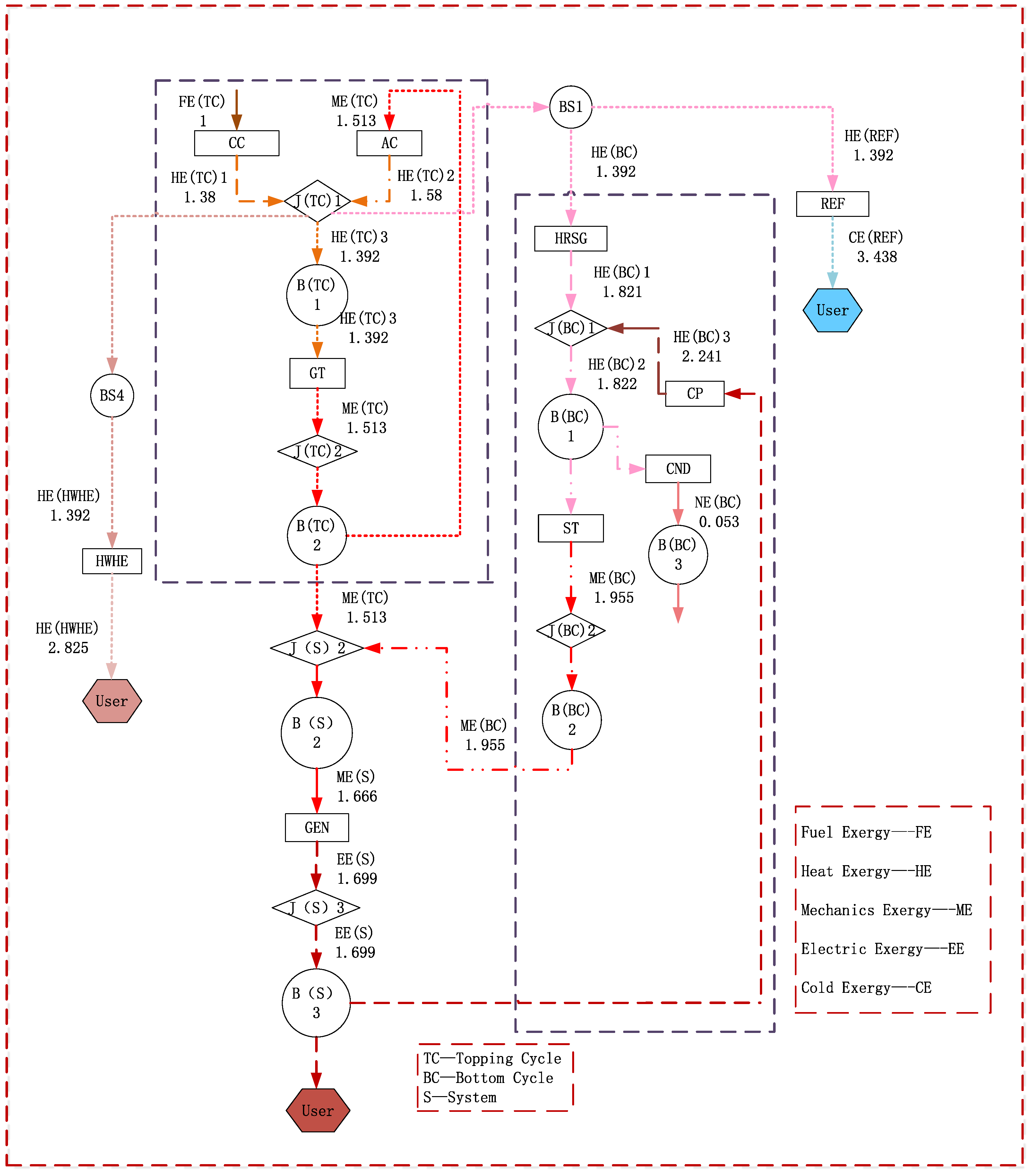
2.1. The Logical Topology Structure Construction Based on the Exergy Flow Attribute Classification

Based on the exergy flow attribute classification, the logical topology structure construction mainly consists of the following five parts: (1) system fuel input, including coal, natural gas, photovoltaic, wind power, and the external grid power supply, represented by a solid line; (2) energy conversion components, including steam turbines, gas turbines, coal-fired boilers, gas boilers, electric refrigerators, absorption chillers, and heat exchangers, and energy conversion components essential to complete a certain thermal cycle, represented by rectangles; (3) thermal cycle components, including gas turbine unit cycles, Rankine cycles, organic Rankine cycles, gas turbine engine cycles, refrigeration cycles, etc., and thermal cycles representing a complete energy conversion (production) closed thermal process, represented by ellipses; (4) energy collection and distribution, based on collection and branch components represented by diamonds and circles, respectively; (5) energy transmission. The energy transfer process is represented by exergy flow, indicated by a dotted line. The process of energy transmission, transformation, and cascade utilization can be displayed intuitively and clearly through the construction of logical topology.

For IESs, the modular construction idea is adopted. The component is taken as the analysis object to analyze the exergy flow classification in the thermal cycle. On the other hand, the thermal cycle is applied as the analysis object, and the energy cascade utilization relationship is used as the basis to analyze and complete the exergy flow classification in the system. The construction of the overall logical topology of the IES can lay a foundation for the graphical modeling of exergy costs. The modular construction process is as follows.

2.1.1. Exergy Flow Classification in the Thermal Cycle

The energy conversion equipment in the thermal cycle is defined as an energy conversion component. Its input and output exergy flow attribute classification is analyzed. According to the function of energy conversion components, the exergy flow attribute classification is conducted, and the exergy flow collection module of the same attribute is established. The number of collection components and branch components is determined by the number of exergy flow attribute categories. Moreover, the collection component is taken as the core to determine the connection relationship between each component within the thermodynamic cycle. The energy conversion component is connected with the corresponding collection component according to its output exergy flow attribute, and the output exergy flow of the collection component under the same attribute is the input exergy flow of the branch component under this attribute.

Figure 1 is a schematic diagram of the exergy flow classification connection in a thermal cycle system. If the input and output exergy attributes of energy conversion components are divided into three categories, i.e., thermal exergy, mechanical exergy, and electrical exergy, the number of collection components and branch components is 3, namely, thermal exergy collection component J1, mechanical exergy collection component J2, and electrical exergy collection component J3. Corresponding branch components are set with the collection components. The corresponding branch components are denoted as thermal exergy branch component B1, mechanical exergy branch component B2, and electrical exergy branch component B3, responsible for thermal exergy, mechanical exergy, and electrical exergy, respectively.

For an energy conversion component with thermal exergy output, the thermal exergy it produces is the input of J1. For an energy conversion component with mechanical exergy output, the mechanical exergy it produces is the input of J2. For an energy conversion component with electrical exergy output, the electrical exergy it produces is the input of J3. In addition, the output of J1 is the only input of B1. The output of J2 is the only input of B2. The output of J3 is the only input of B3.

2.1.2. Exergy Flow Classification in System

In an IES, a variety of prime movers and energy conversion equipment are used to form different thermal cycle processes; various types of energy products can be output to users and realize energy cascade utilization. With the increase in system coupling links, exergy classification of coupling links should be considered in the system.

Firstly, the relationship of energy cascade utilization among thermal cycles in the system is analyzed. The number of coupling nodes is determined by the number of waste heat utilization processes. The exergy flow attribute of each coupling node indicates different levels of thermal exergy. Secondly, each thermal cycle process is defined as a thermal cycle component. According to the function of thermal cycle components, the exergy flow attribute classification is completed, and the exergy flow collection module of the same attribute is established. The number of collection components and branch components is determined by the number of exergy flow attribute categories. Finally, taking the thermal cycle component as the core, the connection relationship of each component in the system is determined. The thermal cycle component is connected with the corresponding collection component according to its output exergy flow attribute, and the output exergy flow of the collection component under the same attribute is the input exergy flow of the branch component under this attribute.

Figure 2 is a schematic diagram of the exergy flow classification connection in the system. The number of waste heat utilization processes and the number of coupling nodes are both 2. In addition to BS1, there are also coupling node branch components BS11 and BS12 corresponding to thermal exergy collection component JS1 in the system. When the input and output exergy attributes of thermal cycle components are divided into three categories, i.e., thermal exergy, electrical exergy, and cold exergy, the number of collection components and branch components is 3, namely thermal exergy collection component JS1, electrical exergy collection component JS2, and cold exergy collection component JS3. Corresponding branch components are set with the collection components. The corresponding branch components are called thermal exergy branch component BS1, electrical exergy branch component BS2, and cold exergy branch component BS3, respectively responsible for thermal exergy, electrical exergy, and cold exergy.

For a thermal cycle component with thermal exergy output, the thermal exergy it produces is the input of JS1. For a thermal cycle component with electrical exergy output, the electrical exergy it produces is the input of JS2. For a thermal cycle component with cold exergy output, the cold exergy it produces is the input of JS3. In addition, the output of JS1 is the only input of BS1. The output of JS2 is the only input of BS2. The output of JS3 is the only input of BS3.

2.2. Exergy Cost Modeling Method Based on Exergy Flow Attribute Classification

According to the logical topology of the system, the exergy cost modeling criteria of input exergy flow, output exergy flow, and coupling link are defined respectively.

2.2.1. Exergy Cost Modeling Criteria of Input Exergy Flow

(1) For a component with external resources, the exergy cost of input exergy flow is 1, as shown in Equation (1):

$$k_{FBn}^{*}=1$$

(1)

where $k_{FBn}^{*}$ is the input exergy flow exergy cost of component n, kW/kW.

(2) For an energy conversion component with different exergy attributes, the exergy cost of input exergy flow is equal to the output exergy cost of branching m, as shown in Equation (2):

$$k_{FBn}^{*}=k_{Pm}^{*}$$

(2)

where $k_{Pm}^{*}$ is the output exergy flow exergy cost of branching m, kW/kW.

2.2.2. Exergy Cost Modeling Criteria of Output Exergy Flow

(1) For the energy conversion component, the output exergy flow exergy cost is equal to the input exergy flow exergy cost of components multiplied by unit exergy consumption, as shown in Equation (3):

$$k_{pn}^{*}=k{B}_n{k}_{FBn}^{*}$$

(3)

where $k_{pn}^{*}$ is the output exergy flow exergy cost of the energy conversion component, kW/kW; $k{B}_n$ is the unit exergy consumption, kW/kW.

(2) For the collection component, the output exergy flow exergy cost is equal to the sum of the input exergy flow exergy cost of each collection tributary multiplied by its exergy flow rate, as shown in Equation (4):

$$k_{pn}^{*}={\displaystyle \sum r_i}{k}_{FBn}^{*}$$

(4)

where $r_i$ is the exergy flow rate.

(3) For the branch component, the output exergy flow exergy cost is equal to the input exergy flow exergy cost $k_{FB}^{*}$, as shown in Equation (5):

$$k_{pn}^{*}=k_{FBn}^{*}$$

(5)

3. Calculation of Irreversible Cost Based on Exergy Flow Attribute Classification

3.1. Existing Irreversible Loss Index Based on Exergy Analysis

Irreversibility exists in all thermal processes and is an important factor for the decrease in system performance. In previous literature, the exergy loss coefficient has been commonly used as the evaluation index to complete the quantitative analysis of the process irreversible loss.

The exergy loss coefficient of the system is

$${\Omega }_i=I_i/F$$

(6)

where ${\Omega }_i$ is the exergy loss coefficient, kW/kW; $I_i$ is the loss of a certain process, kW; $F$ is the total fuel input into the system, kW.

3.2. Calculation of Irreversible Loss Cost Based on Exergy Attribute Classification

In thermoeconomics, energy and funds are collectively referred to as resources. The generation of energy flow in an IES requires the consumption of external resources. The exergy cost modeling method based on exergy attribute classification has some new extensions to the exergy cost theory. The focus of this research is to analyze the influence of irreversible loss accumulation and transfer across the thermal cycle process on the formation of exergy cost.

3.2.1. Analysis of the Relationship between Exergy Cost and Irreversible Cost Based on Exergy Attribute Classification

Based on disturbance theory, the impact of irreversible increases in external resource consumption by each component needs to be evaluated [16] (Valero et al. (1993)), and the fuel effect formula was proposed for the first time in [27,28,29,30,31,32,33,34,35] (Valero and Torres et al.). Further research has been performed on this basis. The basic idea is to obtain the incremental form of external resource consumption from the mathematical form of overall resource consumption. The study focuses on the analysis of irreversible loss increments and further obtains the expression of irreversible cost by linear transformation <KP> matrix.

When the exergy attribute classification method is adopted, the coefficient of technical products is equal to the unit exergy consumption of components, after the exergy of the same attribute is collected. At this time, the diagonal matrix ($n\hspace{0.33em}\times \hspace{0.33em}n$) $〈\mathrm{KP}〉$ containing the coefficient of technical product $k_{ij}$ in the system becomes an n-dimensional vector containing the unit exergy consumption of the exergy conversion component.

According to the exergy balance principle of the system, the increased fuel consumption is converted into an irreversible increase inside the system and an increase in the final product of the system. When the exergy attribute classification method is adopted, after the exergy of the same attribute is collected, the (n × 1) vector ${\mathrm{P}}_{\mathrm{s}}$ containing the final product of the system in the system becomes a scalar $\omega$. From this, an expression of irreversible cost can be obtained, as shown in Equations (7) and (10):

$$I^{*}=\left|\mathrm{I}\right.〉=\mathrm{I}/{\mathrm{P}}_{\mathrm{s}}$$

(7)

where ${\mathrm{P}}_{\mathrm{s}}$ is the (n × 1) vector containing the final product $B_{i0}$ of the system. The irreversible cost and exergy cost of the classified product have the following relationship:

$$k_{p,i}^{*}=1+{\displaystyle \sum _{i=1}^n{I}_i^{*}}$$

(8)

where $k_{p,i}^{*}$ is the exergy cost of the ith exergy flow, kW/kW; $I_i^{*}$ is the irreversible cost of obtaining the ith exergy flow, kW/kW.

A detailed demonstration process is shown in Appendix A.

This equation characterizes the relationship between the exergy cost and the irreversible process cost necessary to obtain the exergy. The formation of the exergy cost of the entire energy conversion process reflects the accumulation of the irreversible cost of the process. With the change in the progressive exergy properties of the system energy conversion process, the exergy cost presents a gradually increasing trend.

3.2.2. Calculation of Irreversible Cost Based on Exergy Flow Attribute Classification

From the analysis of the relationship between exergy cost and irreversible cost based on exergy attribute classification, it can be seen that the exergy cost based on exergy attribute classification can be used to quantify the process impact of process irreversibility on the formation of the final cost of the system. In the same way, through equation deformation, the exergy cost difference can be calculated to obtain the process’s irreversible loss, which converted to external fuel conversion cost (hereafter, this term will be abbreviated as “irreversible cost”). From Equation (8), we can see that

$$k_{p,i+1}^{*}=1+{\displaystyle \sum _{i=1}^n{I}_{i+1}^{*}}=1+{\displaystyle \sum _{i=1}^n{I}_i^{*}}+I_{i+1}^{*}=k_{p,i}^{*}+I_{i+1}^{*}$$

(9)

and we can then obtain the following:

$$I_{i+1}^{*}=k_{p,i+1}^{*}-k_{p,i}^{*}$$

(10)

Equation (10) shows that the irreversible loss cost is equal to the cost difference between adjacent exergy flows after classification, and the irreversible loss cost can be obtained through the calculation of exergy cost.

4. Analysis of Examples

4.1. Typical Integrated Energy System Parameters under Rated Conditions

Take the typical integrated energy system as an example, as shown in Figure 3. It is mainly composed of a gas turbine unit cycle system (topping cycle), Rankine cycle system (bottom cycle), flue gas absorption chiller and hot water heat exchanger, with rated power generation of 389 MW, rated cooling capacity of 11,000 kW and rated heat capacity of 800 kW. After the air is compressed by the air compressor (AC), the air is burned in the combustion chamber (CC) with natural gas. The fuel releases chemical energy to form high-temperature flue gas. The flue gas drives the gas turbine (GT) to perform work, convert heat energy into mechanical energy, and drive the generator (GEN) to generate power. The temperature of the gas discharged from the gas turbine is as high as 583 °C and still has high energy. A portion of these high-temperature gases is sent to the waste heat boiler (HRSG) to heat water into steam to drive the steam turbine (ST) to do work, then drive the generator to generate electricity. The other part enters the absorption refrigerator (REF) for refrigeration, then enters the hot water heat exchanger (HWHE) to recover the waste heat and produce hot water, and is finally discharged into the atmosphere.

The design working condition parameters and calculation conditions are shown in

Table 1. Design working condition parameters and calculation conditions.

Item	Parameters	Values
Apical circulation (gas turbine device cycle)	Atmospheric pressure (kPa)	101.1
	Ambient temperature (°C)	17.4
	Compressor pressure ratio	15.4
	Low calorific value of natural gas (kJ/kg)	48,686.3
	Isentropic efficiency of compressor (%)	85
	Isentropic efficiency of gas turbine (%)	80.7
Bottom circulation (Rankine cycle)	Steam turbine inlet temperature (°C)	565.5
	Steam turbine inlet pressure (kPa)	9563
	Steam turbine exhaust pressure (kPa)	5.96
	Generator efficiency (%)	98
REF	Inlet flue gas temperature (°C)	583.6
	Outlet flue gas temperature (°C)	175
	Inlet temperature of refrigerant water (°C)	12
	Outlet temperature of refrigerant water (°C)	7
	Cooling water inlet temperature (°C)	32
	Cooling water outlet temperature (°C)	36
	Condensation temperature (°C)	39
	Energy efficiency of heat exchanger (%)	85
HWHE	Inlet flue gas temperature (°C)	175
	Outlet flue gas temperature (°C)	90.6
	Inlet water temperature (°C)	50
	Outlet water temperature (°C)	65
System	Rated power generation (MW)	389
	Rated cooling capacity (kW)	11,000
	Rated heat capacity (kW)	800

. The main parameters of each stream under rated conditions are shown in

Table 2. Main parameters of each stream under rated conditions.

Number	m/ (t/h)	P/ (kPa)	T/ (°C)	h/ (kJ/kg)	ex/ (kJ/kg)
1	2270.2	101.1	17.4	42.3	0
2	2270.2	1556.9	422.2	456.9	398.716
3	2329.9	1533.6	1273.2	1494.3	1237.621
4	2329.9	104.4	607.1	693.8	368.278
5	2307.4	101.1	83.8	64.8	26.998
6	280.9	9563	565.5	3542.2	1557.956
7	361	5.857	35.7	2418.6	134.616
8	395	5.856	35.7	149.7	0.168
9	395	2460	36.1	153.2	2.351
10	22.49	101.1	583.6	631.8	257.32
11	22.49	101.1	175	94.8	59.314
12	22.49	101.1	90.6	66.12	29.32
13	1939.32	101.1	12	50.506	0.067
14	1939.32	101.1	7	29.525	0.997
15	43.54	101.1	50	209.42	7.117
16	43.54	101.1	65	272.18	14.719

. The composition of natural gas is shown in

Table 3. Composition of natural gas.

Name	Mole Percentage (%)
Methane	97.6%
Ethane	0.62%
Propane	0.41%
Butane	0.21%
Pentane	0.01%
Hexane	0.05%
Carbon Dioxide	0.65%
Nitrogen	0.45%

.

4.2. Establishment of the Integrated Calculation Model of Exergy Cost and Irreversible Loss Cost Based on Exergy Flow Attribute Classification

According to Section 2, the integrated calculation model of exergy cost and irreversible loss cost based on exergy flow attribute classification was established, and the cost equations are as shown in

Table 4. Exergy cost equations.

	Exergy Cost Modeling of Exergy Flow	Exergy Flow Attribute Classification	Exergy Cost Equations
Topping Cycle (Gas Turbine Device Cycle)	Input exergy flow exergy cost modeling	Input fuel exergy components CC	$k_{FB}^{*}=1$
		Input heat exergy components GT	$k_{FBn}^{*}=k_{PbTC1}^{*}$
		Input mechanics exergy components AC	$k_{FBn}^{*}=k_{PbTC2}^{*}$
	Output exergy flow exergy cost modeling	Components AC, CC and GT	$k_{pn}^{*}=k{B}_n{k}_{FBn}^{*}$
		Join components J(TC)1 and J(TC)2	$k_{pn}^{*}=\sum r_i{k}_{FBn}^{*}$
		Branch components B(TC)1 and B(TC)2	$k_{pn}^{*}=k_{FBn}^{*}$
Bottoming Cycle (Rankine Cycle)	Input exergy flow exergy cost modeling	Input fuel exergy components HRSG	$k_{FBn}^{*}=k_{Pbs1}^{*}$
		Input heat exergy components ST	$k_{FBn}^{*}=k_{PbBC1}^{*}$
	Output exergy flow exergy cost modeling	Components HRSG, CND, ST and GEN	$k_{pn}^{*}=k{B}_n{k}_{FBn}^{*}$
		Join components J(BC)1 and J(BC)2	$k_{pn}^{*}=\sum r_i{k}_{FBn}^{*}$
		Branch components B(BC)1 and B(BC)2	$k_{pn}^{*}=k_{FBn}^{*}$
System	Input exergy flow exergy cost modeling	Input mechanics exergy components GEN	$k_{FBn}^{*}=k_{Pbs2}^{*}$
		Input heat exergy components REF	$k_{FBn}^{*}=k_{Pbs1}^{*}$
		Input heat exergy components HWHE	$k_{FBn}^{*}=k_{Pbs4}^{*}$
	Output exergy flow exergy cost modeling	Join components J(S)1, J(S)2, J(S)3 and J(S)4	$k_{pn}^{*}=\sum r_i{k}_{FBn}^{*}$
		Branch components B(S)1, B(S)2, B(S)3 and B(S)4	$k_{pn}^{*}=k_{FBn}^{*}$
		Output electric exergy components GEN	$k_{pn}^{*}=k{B}_n{k}_{FBn}^{*}$
		Output cooling exergy components REF	$k_{pn}^{*}=k{B}_n{k}_{FBn}^{*}$
		Output heat exergy components HWHE	$k_{pn}^{*}=k{B}_n{k}_{FBn}^{*}$

.

4.3. Analysis of Exergy Cost and Irreversible Loss Cost Distribution

Using the above modeling method, the cost of the integrated energy system is calculated. The fuel-product calculation results for the integrated energy system under rated conditions are shown in

Table 5. Fuel-product calculation for the integrated energy system under rated conditions.

Component *		Fuel Exergy Consumption	Product	Unit Exergy Consumption	Exergy Flow Rate
		FB (kW)	P (kW)	kBn (kW/kW)	r
1	AC	261,432.5	251,434.8	1.04	0.060
2	CC	718,204.1	529,022.4	1.36	0.940
3	GT	562,633.6	518,127.6	1.09	0.654
4	HRSG	219,357	168,359.1	1.30	0.999
5	ST	151,210.12	141,167.47	1.07	0.346
6	CND	6280.34	214,884.5	0.03	-
7	CP	384.03	239.52	1.60	0.001
8	GEN	395,678.8	387,765.3	1.02	-
9	REF	1237	500.991	2.47	-
10	HWHE	187.41	91.95	2.03	-

Note *: Common component fuel-product definitions are given in references [36].

.

The exergy cost equations given in Table 4 are solved by Seidel iterative method; the calculation results are shown in Figure 4 and Figure 5 and

Table 6. Exergy cost of exergy flow with different attributes.

Exergy Cost ${\mathit{k}}_{\mathit{p}}^{*}$ (KW/KW)		FE	HE	ME	EE	CE	HE
Topping Cycle		1	1.392	1.513
Bottoming Cycle			1.392	1.955
System	GEN			1.666	1.699
	REF		1.392			3.438
	HWHE		1.392				2.825

.

As shown in Figure 4, Figure 5 and Table 6, in the process of conversion from fuel exergy to electric exergy, heat exergy and cold exergy, the cost of exergy flow with different attributes increases with the increase in irreversible links. Fuel exergy cost 1 kW/kW increases to terminal mechanical exergy cost 1.513 kW/kW in the topping cycle. Heat exergy cost 1.392 kW/kW increases to terminal mechanical exergy cost 1.955 kW/kW in the bottoming cycle.

In the system, after the mechanical exergy of the topping cycle and the bottoming cycle is collected, the mechanical exergy cost of the system is 1.666 kW/kW, increasing to terminal electric exergy cost 1.699 kW/kW. Heat exergy (REF) cost 1.392 kW/kW increases to terminal cold exergy cost 3.438 kW/kW. Heat exergy (HWHE) cost 1.392 kW/kW increases to terminal heat exergy cost 2.825 kW/kW.

As shown in Figure 6 and

Table 7. Irreversible loss cost of exergy flow with different attributes.

Irreversible Loss Cost ${\mathit{I}}^{*}$ (KW/KW)		FE-HE	HE-HE	HE-ME	ME-EE	HE-CE	HE-HE
Topping Cycle		0.392		0.121
Bottoming Cycle			0.429	0.134
System	GEN				0.033
	REF					2.046
	HWHE						1.433

, the exergy cost difference of adjacent different attribute exergy flows in the thermal cycle is the irreversible loss of the production process itself. The exergy cost is composed of the accumulated irreversible costs of each link.

The energy conversion process from fuel to heat FE(TC)—HE(TC), HE(BC)—HE(BC)1, HE(REF)—CE(REF) and HE(HWHE)—HE(HWHE) produces a higher irreversible cost. Due to the inequivalence of process irreversibility loss, we should pay attention to the energy conversion processes with a high irreversible cost.

In the process of energy conversion, with the accumulation of irreversible loss, the exergy cost of exergy flow with different attributes increases. An example is given to analyze the relationship between the increase in irreversible loss and increase in cost, and the transfer process of irreversible loss across thermal cycles is given. Due to the transmission and coupling of the irreversible cost in each energy conversion link, the mechanism of exergy cost formation can be obtained by the distribution diagram of the exergy flow cost and the irreversible cost.

5. Conclusions

An IES provides an important pathway to realize energy cascade utilization. Developing suitable thermodynamic analysis methodologies is important for IES assessment and optimization. This paper proposes an irreversible cost and exergy cost integrated analysis method for IESs based on improved thermoeconomics, in which linear transformation of the <KP> matrix is applied to unify the process irreversible loss and the exergy cost of the system together. A case study on a 389MW combined cooling, heating and power IES shows that: (1) IES exergy costs increase with the accumulation of irreversible losses. The combustion process and the conversion process from high-quality energy into low-quality energy have the highest irreversible losses, which lead to a substantial increase in exergy costs. (2) In the process of energy cascade utilization, the accumulation of irreversible losses in the upstream cycle will be transferred to the downstream through the interaction, which will influence the exergy costs of downstream products. The proposed approach can provide deep insight into the formation of exergy costs within a polygeneration system and characterize processes of irreversible loss across thermal cycles and energy cascade utilization, thus revealing the weak links in an IES and offering directions for system performance improvements. This study focused on energy loss and energy grade decline, thus analyzing the position of the maximum irreversible loss of the system. If more advanced equipment is used, the equipment costs should not be ignored. Considering the cost of the equipment, thermoeconomic costs in price terms will be our future research interest.

References

1. Köse, Ö.; Koç, Y.; Yağlı, H. Performance improvement of the bottoming steam Rankine cycle (SRC) and organic Rankine cycle (ORC) systems for a triple combined system using gas turbine (GT) as topping cycle. Energy Convers. Manag. 2020, 211, 112745. [Google Scholar] [CrossRef]
2. Xi, H.; Wu, X.; Chen, X.; Sha, P. Artificial intelligent based energy scheduling of steel mill gas utilization system towards carbon neutrality. Appl. Energy 2021, 295, 117069. [Google Scholar] [CrossRef]
3. Memon, A.G.; Memon, R.A.; Qureshi, S. Thermo-environmental and economic analyses of combined cycle power plants with regression modelling and optimization. Appl. Therm. Eng. 2017, 125, 489–512. [Google Scholar] [CrossRef]
4. Wu, X.; Xi, H.; Ren, Y.; Lee, K.Y. Power-Carbon Coordinated Control of BFG-Fired CCGT Power Plant Integrated with Solvent-based Post-Combustion CO2 Capture. Energy 2021, 226, 120435. [Google Scholar] [CrossRef]
5. Postnikov, I.; Stennikov, V.; Penkovskii, A. Integrated Energy Supply Schemes on Basis of Cogeneration Plants and Wind Power Plants. Energy Procedia 2019, 158, 154–159. [Google Scholar] [CrossRef]
6. Chen, X.; Wu, X.; Lee, K.Y. The mutual benefits of renewables and carbon capture: Achieved by an artificial intelligent scheduling strategy. Energy Convers. Manag. 2021, 233, 113856. [Google Scholar] [CrossRef]
7. Kler, A.M.; Potanina, Y.M.; Marinchenko, A.Y. Co-optimization of thermal power plant flowchart, thermodynamic cycle parameters, and design parameters of components. Energy 2020, 193, 116679. [Google Scholar] [CrossRef]
8. Zhu, M.; Wu, X.; Shen, J.; Lee, K. Dynamic modeling, validation and analysis of direct air-cooling condenser with integration to the coal-fired power plant for flexible operation. Energy Convers. Manag. 2021, 245, 114601. [Google Scholar] [CrossRef]
9. Chen, Q.; Han, W.; Zheng, J.-J.; Sui, J.; Jin, H.-G. The exergy and energy level analysis of a combined cooling, heating and power system driven by a small scale gas turbine at off design condition. Appl. Therm. Eng. 2014, 66, 590–602. [Google Scholar] [CrossRef]
10. Jie, P.; Yan, F.; Wen, Z.; Li, J. Evaluation of the biomass gasification-based combined cooling, heating and power system using the maximum generalized entropy principle. Energy Convers. Manag. 2019, 192, 150–160. [Google Scholar] [CrossRef]
11. Wang, J.; Chen, Y.; Dou, C.; Gao, Y.; Zhao, Z. Thermodynamic performance analysis and comparison of a combined cooling heating and power system integrated with two types of thermal energy storage. Energy 2018, 163, 475–489. [Google Scholar] [CrossRef]
12. Khan, M.S.; Abid, M.; Ratlamwala, T.A.H. Energy, Exergy and Economic Feasibility Analyses of a 60 MW Conventional Steam Power Plant Integrated with Parabolic Trough Solar Collectors Using Nanofluids. Iran. J. Sci. Technol. Trans. Mech. Eng. 2019, 43, 193–209. [Google Scholar] [CrossRef]
13. Mohammadi, A.; Ahmadi, M.H.; Bidi, M.; Joda, F.; Valero, A.; Uson, S. Exergy analysis of a Combined Cooling, Heating and Power system integrated with wind turbine and compressed air energy storage system. Energy Convers. Manag. 2017, 131, 69–78. [Google Scholar] [CrossRef]
14. Adibhatla, S.; Kaushik, S.C. Energy, exergy and economic (3E) analysis of integrated solar direct steam generation combined cycle power plant. Sustain. Energy Technol. Assess. 2017, 20, 88–97. [Google Scholar] [CrossRef]
15. Cai, Y.; Li, J.; Liu, H.; He, Q. Exergy Analysis of Compressed Air Energy Storage System Combined with Absorption Chiller. Zhongguo Dianji Gongcheng Xuebao/Proc. Chin. Soc. Electr. Eng. 2018, 38, 186–194. [Google Scholar]
16. Lozano, M.A.; Valero, A. Theory of the exergetic cost. Energy 1993, 18, 939–960. [Google Scholar] [CrossRef]
17. Erlach, B.; Serra, L.; Valero, A. Structural theory as standard for thermoeconomics. Energy Convers. Manag. 1999, 40, 1627–1649. [Google Scholar] [CrossRef]
18. Haydargil, D.; Abuşoğlu, A. A comparative thermoeconomic cost accounting analysis and evaluation of biogas engine-powered cogeneration. Energy 2018, 159, 97–114. [Google Scholar] [CrossRef]
19. Marques, A.S.; Carvalho, M.; Ochoa, Á.A.V.; Souza, R.J.; dos Santos, C.A.C. Exergoeconomic assessment of a compact electricity-cooling cogeneration unit. Energies 2020, 13, 5417. [Google Scholar] [CrossRef]
20. Boyaghchi, F.A.; Chavoshi, M. Multi-criteria optimization of a micro solar-geothermal CCHP system applying water/CuO nanofluid based on exergy, exergoeconomic and exergoenvironmental concepts. Appl. Therm. Eng. 2017, 112, 660–675. [Google Scholar] [CrossRef]
21. Ghaffarpour, Z.; Mahmoudi, M.; Mosaffa, A.; Farshi, L.G. Thermoeconomic assessment of a novel integrated biomass based power generation system including gas turbine cycle, solid oxide fuel cell and Rankine cycle. Energy Convers. Manag. 2018, 161, 1–12. [Google Scholar] [CrossRef]
22. Villafana, E.D.S.; Bueno, J.P.V.M. Thermoeconomic and environmental analysis and optimization of the supercritical CO2 cycle integration in a simple cycle power plant. Appl. Therm. Eng. 2019, 152, 1–12. [Google Scholar] [CrossRef]
23. Ameri, M.; Mohammadzadeh, M. Thermodynamic, thermoeconomic and life cycle assessment of a novel integrated solar combined cycle (ISCC) power plant. Sustain. Energy Technol. Assess. 2018, 27, 192–205. [Google Scholar] [CrossRef]
24. Wang, J.; Liu, W.; Meng, X.; Liu, X.; Gao, Y.; Yu, Z.; Bai, Y.; Yang, X. Study on the Coupling Effect of a Solar-Coal Unit Thermodynamic System with Carbon Capture. Energies 2020, 13, 4779. [Google Scholar] [CrossRef]
25. Zhai, R.; Liu, H.; Wu, H.; Yu, H.; Yang, Y. Analysis of Integration of MEA-Based CO2 Capture and Solar Energy System for Coal-Based Power Plants Based on Thermo-Economic Structural Theory. Energies 2018, 11, 1284. [Google Scholar] [CrossRef] [Green Version]
26. Arena, A.P.; Borchiellini, R. Application of different productive structures for thermoeconomic diagnosis of a combined cycle power plant. Int. J. Therm. Sci. 1999, 38, 601–612. [Google Scholar] [CrossRef]
27. Tsatsaronis, G.; Park, M.-H. On avoidable and unavoidable exergy destructions and investment costs in thermal systems. Energy Convers. Manag. 2002, 43, 1259–1270. [Google Scholar] [CrossRef]
28. Valero, A.; Serra, L.; Uche, J. Fundamentals of exergy cost accounting and thermoeconomics. Part I: Theory. J. Energy Resour. Technol. Trans. ASME 2006, 128, 1–8. [Google Scholar] [CrossRef]
29. Torres, C.; Valero, A.; Rangel, V.; Zaleta, A. On the cost formation process of the residues. Energy 2008, 33, 144–152. [Google Scholar] [CrossRef]
30. Valero, A.; Usón, S.; Torres, C.; Stanek, W. Theory of exergy cost and thermo-ecological cost. In Thermodynamics for Sustainable Management of Natural Resources; Stanek, W., Ed.; Springer: Berlin/Heidelberg, Germany, 2017; ISBN 978–3-319–48648–2. [Google Scholar]
31. Torres, C.; Valero, A.; Serra, L.; Royo, J. Structural theory and thermoeconomic diagnosis: Part I. On malfunction and dysfunction analysis. Energy Convers. Manag. 2002, 43, 1503–1518. [Google Scholar] [CrossRef]
32. Valero, A.; Correas, L.; Zaleta, A.; Lazzaretto, A.; Verda, V.; Reini, M.; Rangel, V. On the thermoeconomic approach to the diagnosis of energy system malfunctions. Part 1: The TADEUS problem and Part 2: Malfunction definitions and assessment. Energy 2004, 29, 1875–1907. [Google Scholar] [CrossRef]
33. Usón, S.; Uche, J.; Martínez, A.; del Amo, A.; Acevedo, L.; Bayod, A. Exergy assessment and exergy cost analysis of a renewable-based and hybrid trigeneration scheme for domestic water and energy supply. Energy 2019, 168, 662–683. [Google Scholar] [CrossRef]
34. Valero, A.; Lerch, F.; Serra, L.; Royo, J. Structural theory and thermoeconomic diagnosis: Part II: Application to an actual power plant. Energy Convers. Manag. 2002, 43, 1519–1535. [Google Scholar] [CrossRef]
35. Cuadra, C.T. Symbolic thermoeconomic analysis of energy systems. In Exergy, Energy System Analysis and Optimization: Thermoeconomic Analysis Modeling, Simulation and Optimization in Energy Systems; EOLSS Publishers: Oxford, UK, 2006. [Google Scholar]
36. Torres, C.; Valero, A. The Exergy Cost Theory Revisited. Energies 2021, 14, 1594. [Google Scholar] [CrossRef]
Figure 1. Classification of exergy flow in a thermal cycle.
Processes 10 00137 g001
Figure 2. Classification of exergy flow in the system.
Processes 10 00137 g002
Figure 3. Thermal system diagram of the integrated energy system.
Processes 10 00137 g003
Figure 4. Exergy cost distribution of the IES.
Processes 10 00137 g004
Figure 5. Exergy cost of exergy flow with different attributes.
Processes 10 00137 g005
Figure 6. Irreversible loss cost of exergy flow with different attributes.
Processes 10 00137 g006