Joint Asymptotic Distributions of Smallest and Largest Insurance Claims

Abstract

Assume that claims in a portfolio of insurance contracts are described by independent and identically distributed random variables with regularly varying tails and occur according to a near mixed Poisson process. We provide a collection of results pertaining to the joint asymptotic Laplace transforms of the normalised sums of the smallest and largest claims, when the length of the considered time interval tends to infinity. The results crucially depend on the value of the tail index of the claim distribution, as well as on the number of largest claims under consideration.

1. Introduction

When dealing with heavy-tailed insurance claims, it is a classical problem to consider and quantify the influence of the largest among the claims on their total sum, see e.g., Ammeter [1] for an early reference in the actuarial literature. This topic is particularly relevant in non-proportional reinsurance applications when a significant proportion of the sum of claims is consumed by a small number of claims. The influence of the maximum of a sample on the sum has in particular attracted considerable attention over the last fifty years (see Ladoucette and Teugels [2] for a recent overview of existing literature on the subject). Different modes of convergence of the ratios sum over maximum or maximum over sum have been linked with conditions on additive domain of attractions of a stable law (see e.g., Darling [3], Bobrov [4], Chow and Teugels [5], O’Brien [6] and Bingham and Teugels [7]).

It is also of interest to study the joint distribution of normalised smallest and largest claims. We will address this question in this paper under the assumption that the number of claims over time is described by a rather general counting process. These considerations may be helpful for the design of possible reinsurance strategies and risk management in general. In particular, extending the understanding of the influence of the largest claim on the aggregate sum (which is a classical topic in the theory of subexponential distributions) towards the relative influence of several large claims together, can help to assess the potential gain from reinsurance treaties of large claim reinsurance and ECOMOR type (see e.g., Section 1).

In this paper we consider a homogeneous insurance portfolio, where the distribution of the individual claims has a regularly varying tail. The number of claims is generated by a near mixed Poisson process. For this rather general situation we derive a number of limiting results for the joint Laplace transforms of the smallest and largest claims, as the time t tends to infinity. These turn out to be quite explicit and crucially depend on the rule of what is considered to be a large claim as well as on the value of the tail index.

Let $X_1,X_2,\dots$ be a sequence of independent positive random variables (representing claims) with common distribution function F. For $n\ge 1$, denote by $X_1^{*}\le X_2^{*}\le \dots \le X_n^{*}$ the corresponding order statistics. We assume that the claim size distribution satisfies the condition

$$1-F(x)=\overline{F}(x)=x^{-\alpha }\ell (x),x>0$$

(1)

where $\alpha >0$ and ℓ is a slowly varying function at infinity. The tail index is defined as $\gamma =1/\alpha$ and we will typically express our results in terms of γ. Denote by $U(y)=F^{\leftarrow }(1-1/y)$ the tail quantile function of F where $F^{\leftarrow }\left(t\right)=inf\left\{x\in \mathbb{R}:F\left(x\right)\ge t\right\}$. Under (1), $U(y)=y^{\gamma }{\ell }_1(y)$, where ${\ell }_1$ is again a slowly varying function. For textbook treatments of regularly varying distributions and/or their applications in insurance modelling, see e.g., Bingham et al. [8], Embrechts et al. [9], Rolski et al. [10] and Asmussen and Albrecher [11].

Denote the number of claims up to time t by $N(t)$ with $p_n(t)=P(N(t)=n)$. The probability generating function of $N(t)$ is given by

$$Q_t(z)=E\left\{z^{N(t)}\right\}=\sum _{n=0}^{\infty }{p}_n(t)z^n$$

which is defined for $\left|z\right|\le 1$. Let

$$Q_t^{(r)}(z)=r!E\left\{\left(\begin{array}{c}N(t)\\ r\end{array}\right)z^{N(t)-r}\right\}$$

be its derivative of order r with respect to z. In this paper we assume that $N(t)$ is a near mixed Poisson (NMP) process, i.e., the claim counting process satisfies the condition

$$\frac{N(t)}{t}\stackrel{D}{\to }\Theta ,t\uparrow \infty$$

for some random variable Θ, where D denotes convergence in distribution. This condition implies that

$$Q_t\left(1-\frac{w}{t}\right)\to E\left\{e^{-w\Theta }\right\}$$

(2)

and

$$\frac{1}{t^r}{Q}_t^{(r)}\left(1-\frac{w}{t}\right)\to E\left\{e^{-w\Theta }{\Theta }^r\right\}:=q_r(w),t\uparrow \infty$$

Note also that, for $\beta >0$ and $r\in \mathbb{N}$,

$${\int }_0^{\infty }{w}^{\beta -1}{q}_r(w)dw=\Gamma \left(\beta \right)E\left\{{\Theta }^{r-\beta }\right\}.$$

(3)

A simple example of an NMP process is the homogeneous Poisson process, which is very popular in claims modelling and plays a crucial role in both actuarial literature and in practice. The class of mixed Poisson processes (for which condition (2) holds not only in the limit, but for any t) has found numerous applications in (re)insurance modelling because of its flexibility, its success in actuarial data fitting and its property of being more dispersed than the Poisson process (see Grandell [12] for a general account and various characterisations of mixed Poisson processes). The mixing may, e.g., be interpreted as claims coming from a heterogeneity of groups of policyholders or of contract specifications. The more general class of NMP processes is used here mainly because the results hold under this more general setting as well. The NMP distributions (for fixed t) contain the class of infinitely divisible distributions (if the component distribution has finite mean). Moreover any renewal process generated by an interclaim distribution with finite mean ν is an NMP process (note that then by the weak law of large numbers in renewal theory, $N(t)/t\stackrel{\mathcal{D}}{\to }\Theta$ where Θ is degenerate at the point $1/\nu$).

The aggregate claim up to time t is given by

$$S(t)=\sum _{j=1}^{N(t)}{X}_j$$

where it is assumed that ${\left(N(t)\right)}_{t\ge 0}$ is independent of the claims ${\left(X_i\right)}_{i\ge 1}$. For $s\in \mathbb{N}$ and $N(t)\ge s+2$, we define the sum of the $N(t)-s-1$ smallest and the sum of the s largest claims by

$${\Sigma }_s(t)=\sum _{j=1}^{N(t)-s-1}{X}_j^{*},{\Lambda }_s(t)=\sum _{j=N(t)-s+1}^{N(t)}{X}_j^{*}$$

so that $S(t)={\Sigma }_s(t)+X_{N(t)-s}^{*}+{\Lambda }_s(t)$. Here Σ refers to small while Λ refers to large.

In this paper we study the limiting behaviour of the triplet $({\Lambda }_s(t),X_{N(t)-s}^{*},{\Sigma }_s(t))$ with appropriate normalisation coefficients depending on γ, the tail index, and on s, the number of terms in the sum of the largest claims. We will consider three asymptotic cases, as they show a different behaviour: s is fixed, s tends to infinity but slower than the expected number of claims, and s tends to infinity and is asymptotically equal to a proportion of the number of claims.

Example 1. In large claim reinsurance for the s largest claims in a specified time interval $[0,t]$, the reinsured amount is given by ${\Lambda }_s(t)$, so the interpretation of our results to the analysis of such reinsurance treaties is immediate. A variant of large claim reinsurance that also has a flavour of excess-of-loss treaties is the so-called ECOMOR (excedent du cout moyen relatif) treaty with reinsured amount

$$\sum _{j=N(t)-s+1}^{N(t)}(X_j^{*}-X_{N(t)-s}^{*}),$$

i.e., the deductible is itself an order statistic (or in other words, the reinsurer pays all exceedances over the s-largest claim). This treaty has some interesting properties, for instance with respect to inflation, see e.g., Ladoucette & Teugels [13]. If the reinsurer accepts to only cover a proportion β ($0<\beta <1$) of this amount, the cedent’s claim amount is given by

$${\Sigma }_s(t)+\beta s{X}_{N(t)-s}^{*}+(1-\beta ){\Lambda }_s(t),$$

which is a weighted sum of the quantities ${\Sigma }_s(t)$, $X_{N(t)-s}^{*}$ and ${\Lambda }_s(t)$. The asymptotic results above in terms of the Laplace transform can then be used to approximate the distribution of the cedent’s and reinsurer’s claim amount in such a contract, and correspondingly the design of a suitable contract (including the choice of s) will depend quite substantially on the value of the extreme value index of the underlying claim distribution.

The paper is organised as follows. We first give the joint Laplace transform of the triplet $({\Lambda }_s(t),X_{N(t)-s}^{*},{\Sigma }_s(t))$ for a fixed t in Section 2. Section 3 deals with asymptotic joint Laplace transforms in the case $\gamma >1$. We also discuss consequences for moments of ratios of the limiting quantities. The behaviour for $\gamma =1$ depends on whether $\mathbb{E}\left[X_i\right]$ is finite or not. In the first case, the analysis for $\gamma <1$ applies, whereas in the latter one has to adapt the analysis of Section 3 exploiting the slowly varying function ${\int }_0^{x}ydF(y)$, but we refrain from treating this very special case in detail (see e.g., Albrecher and Teugels [14] for a similar adaptation in another context). Section 4 and Section 5 treat the case $\gamma <1$ without and with centering, respectively. The proofs of the results in Section 3, Section 4 and Section 5 are given in Section 6. Section 7 concludes.

2. Preliminaries

In this section, we state a versatile formula that will allow us later to derive almost all the desired asymptotic properties of the joint distributions of the triplet $({\Lambda }_s(t),X_{N(t)-s}^{*},{\Sigma }_s(t))$. We consider the joint Laplace transform of $({\Lambda }_s(t),X_{N(t)-s}^{*},{\Sigma }_s(t))$ to study their joint distribution in an easy fashion. For a fixed t, it is denoted by

$${\Omega }_s(u,v,w;t)=E\left\{exp(-u{\Lambda }_s(t)-v{X}_{N(t)-s}^{*}-w{\Sigma }_s(t))\right\}.$$

Then the following representation holds:

Proposition 1. We have

$$\begin{array}{cc}\hfill {\Omega }_s(u,v,w;t)=& \sum _{n=0}^s{p}_n(t){\left({\int }_0^{\infty }{e}^{-ux}dF(x)\right)}^n+\hfill \\ & \frac{1}{s!}{\int }_0^{\infty }{\left(E\left[1_{\{X>y\}}{e}^{-uX}\right]\right)}^s{e}^{-vy}{Q}_t^{(s+1)}\left(E\left\{1_{\{X<y\}}{e}^{-wX}\right\}\right)dF(y).\hfill \end{array}$$

Proof. The proof is standard if we interpret $X_r^{*}=0$ whenever $r\le 0$. Indeed, condition on the number of claims at the time epoch t and subdivide the requested expression into three parts:

$$\begin{array}{ccc}\hfill {\Omega }_s(u,v,w;t)& =& \sum _{n=0}^s{p}_n(t)E\left\{exp\left(\left.-u\sum _{j=1}^n{X}_j\right|N(t)=n\right)\right\}\hfill \\ & & +p_{s+1}(t)E\left\{exp\left(\left.-u\sum _{j=2}^{s+1}{X}_j^{*}-v{X}_1^{*}\right|N(t)=s+1\right)\right\}\hfill \\ & & +\sum _{n=s+2}^{\infty }{p}_n(t)E\left\{exp\left(\left.-u\sum _{j=n-s+1}^n{X}_j^{*}-v{X}_{n-s}^{*}-w\sum _{j=1}^{n-s-1}{X}_j^{*}\right|N(t)=n\right)\right\}\hfill \end{array}$$

The conditional expectation in the first term on the right simplifies easily to the form ${({\int }_0^{\infty }{e}^{-ux}dF(x))}^n$. For the conditional expectations in the second and third term, we condition additionally on the value y of the order statistic $X_{n-s}^{*}$; the $n-s-1$ order statistics $X_1^{*},X_2^{*},\dots ,X_{n-s-1}^{*}$ are then distributed independently and identically on the interval $[0,y]$ yielding the factor ${({\int }_0^y{e}^{-wx}dF(x))}^{n-s-1}$. A similar argument works for the s order statistics $X_{n-s+1}^{*},X_{n-s+2}^{*},\dots ,X_n^{*}$. Combining the two terms yields

$$\begin{array}{cc}\hfill {\Omega }_s(u,v,w;t)=& \sum _{n=0}^s{p}_n(t){\left({\int }_0^{\infty }{e}^{-ux}dF(x)\right)}^n\hfill \\ & +\sum _{n=s+1}^{\infty }{p}_n(t)\frac{n!}{s!(n-s-1)!}{\int }_0^{\infty }{\left({\int }_y^{\infty }{e}^{-ux}dF(x)\right)}^s{e}^{-vy}{\left({\int }_0^y{e}^{-wx}dF(x)\right)}^{n-s-1}dF(y).\hfill \end{array}$$

A straightforward calculation finally shows

$$\begin{array}{cc}\hfill {\Omega }_s(u,v,w;t)=& \sum _{n=0}^s{p}_n(t){\left({\int }_0^{\infty }{e}^{-ux}dF(x)\right)}^n+\hfill \\ & \frac{1}{s!}{\int }_0^{\infty }{\left({\int }_y^{\infty }{e}^{-ux}dF(x)\right)}^s{e}^{-vy}{Q}_t^{(s+1)}\left({\int }_0^y{e}^{-wx}dF(x)\right)dF(y).\hfill \end{array}$$

  ☐

Consequently, it is possible to easily derive the expectations of products (or ratios) of ${\Lambda }_s(t)$, $X_{N(t)-s}^{*}$, ${\Sigma }_s(t)$ and $S(t)$ by differentiating (or integrating) the joint Laplace transform. We only write down their first moment for simplicity.

Corollary 2. We have

$$\begin{array}{ccc}\hfill E\left\{{\Lambda }_s(t)\right\}& =& \sum _{n=1}^{s}n{p}_n(t)E\left\{X_1\right\}+\frac{1}{(s-1)!}{\int }_0^{\infty }{\left(\overline{F}(y)\right)}^{s-1}\left({\int }_y^{\infty }xdF(x)\right)Q_t^{(s+1)}\left(F(y)\right)dF(y)\hfill \\ \hfill E\left\{X_{N(t)-s}^{*}\right\}& =& \frac{1}{s!}{\int }_0^{\infty }y{\left(\overline{F}(y)\right)}^s{Q}_t^{(s+1)}\left(F(y)\right)dF(y)\hfill \\ \hfill E\left\{{\Sigma }_s(t)\right\}& =& \frac{1}{s!}{\int }_0^{\infty }{\left(\overline{F}(y)\right)}^s{Q}_t^{(s+2)}\left(F(y)\right)\left({\int }_0^{y}xdF(x)\right)dF(y)\hfill \\ \hfill E\left\{S(t)\right\}& =& E\left\{N(t)\right\}E\left\{X_1\right\}\hfill \end{array}$$

Proof. The individual Laplace transforms can be written in the following form:

$$\begin{array}{ccc}\hfill E\left\{exp(-u{\Lambda }_s(t)\right\}& =& \sum _{n=0}^s{p}_n(t){\left({\int }_0^{\infty }{e}^{-ux}dF(x)\right)}^n\hfill \\ & & +\frac{1}{s!}{\int }_0^{\infty }{\left({\int }_y^{\infty }{e}^{-ux}dF(x)\right)}^s{Q}_t^{(s+1)}\left(F(y)\right)dF(y)\hfill \\ \hfill E\left\{exp(-v{X}_{N(t)-s}^{*}\right\}& =& {\Pi }_{s+1}(t)+\frac{1}{s!}{\int }_0^{\infty }{\left(\overline{F}(y)\right)}^s{e}^{-vy}{Q}_t^{(s+1)}\left(F(y\right))dF(y)\hfill \\ \hfill E\left\{exp(-w{\Sigma }_s(t)\right\}& =& {\Pi }_{s+1}(t)+\frac{1}{s!}{\int }_0^{\infty }{\left(\overline{F}(y)\right)}^s{Q}_t^{(s+1)}\left({\int }_0^y{e}^{-wx}dF(x)\right)dF(y)\hfill \\ \hfill E\left\{exp(-uS(t)\right\}& =& Q_t\left({\int }_0^{\infty }{e}^{-ux}dF(x)\right),\hfill \end{array}$$

where ${\Pi }_{s+1}(t)={\sum }_{n=0}^s{p}_n(t)$. By taking the first derivative, we arrive at the respective expectations.     ☐

3. Asymptotics for the Joint Laplace Transforms when $\gamma >1$

Before giving the asymptotic joint Laplace transform of the sum of the smallest and the sum of the largest claims, we first recall an important result about convergence in distribution of order statistics and derive a characterisation of their asymptotic distribution. All proofs of this section are deferred to Section 6.

It is well-known that there exists a sequence $E_1,E_2,\dots$ of exponential random variables with unit mean such that

$$(X_n^{*},\dots ,X_1^{*})\stackrel{D}{=}\left((U\left({\Gamma }_{n+1}/{\Gamma }_1\right),\dots ,U\left({\Gamma }_{n+1}/{\Gamma }_n\right)\right),$$

where ${\Gamma }_k=E_1+\dots +E_k$. Let $Z_n=\left(X_n^{*},\dots ,X_1^{*},0,\dots \right)/U(n)$. It may be shown that $Z_n$ converges in distribution to $Z=\left(Z_1,Z_{2,}\dots \right)$ in ${\mathbb{R}}_{+}^{\mathbb{N}}$, where $Z_k={\Gamma }_k^{-\gamma }$ (see Lemma 1 in LePage et al. [15]). For $\gamma >1$, the series ${({\sum }_{k=1}^n{\Gamma }_k^{-\gamma })}_{n\ge 1}$ converges almost surely. Therefore, for a fixed s, we deduce that, as $n\to \infty$,

$$\left(\sum _{j=n-s+1}^n{X}_j^{*},X_{n-s}^{*},\sum _{j=1}^{n-s-1}{X}_j^{*}\right)/U(n)\stackrel{D}{\to }\left(\sum _{k=1}^s{\Gamma }_k^{-\gamma },{\Gamma }_{s+1}^{-\gamma },\sum _{k=s+2}^{\infty }{\Gamma }_k^{-\gamma }\right).$$

(4)

In particular, we derive by the Continuous Mapping Theorem that

$$\frac{{\sum }_{j=1}^{n-s}{X}_j^{*}}{X_{n-s}^{*}}\stackrel{D}{\to }{R}_{(s)}=\frac{{\sum }_{k=s+1}^{\infty }{\Gamma }_k^{-\gamma }}{{\Gamma }_{s+1}^{-\gamma }}.$$

Note that the first moment of $R_{(s)}$ (but only the first moment) may be easily derived since

$$E\left\{R_{(s)}\right\}=1+\sum _{j=s+2}^{\infty }E\left\{B_j^{\gamma }\right\}=1+\frac{s+1}{\gamma -1},$$

(5)

where $B_j={\sum }_{i=1}^{s+1}{E}_i/{\sum }_{i=1}^j{E}_i$ has a Beta$\left(s+1,j-1\right)$ distribution. We also recall that F belongs to the (additive) domain of attraction of a stable law with index $\gamma >1$ if and only if

$$\underset{n\to \infty }{lim}E\left\{\frac{{\sum }_{j=1}^n{X}_j^{*}}{X_n^{*}}\right\}=E\left\{R_{(0)}\right\}=1+\frac{1}{\gamma -1}=\frac{1}{1-1/\gamma }$$

(see e.g., Theorem 1 in Ladoucette and Teugels [2]).

When ${\left(N(t)\right)}_{t\ge 0}$ is an NMP process, we also have, as $t\to \infty$,

$$\left(\sum _{j=N(t)-s+1}^{N(t)}{X}_j^{*},X_{N(t)-s}^{*},\sum _{j=1}^{N(t)-s-1}{X}_j^{*}\right)/U(N(t))\stackrel{D}{\to }\left(\sum _{k=1}^s{\Gamma }_k^{-\gamma },{\Gamma }_{s+1}^{-\gamma },\sum _{k=s+2}^{\infty }{\Gamma }_k^{-\gamma }\right)$$

(6)

and

$$\frac{{\sum }_{j=1}^{N(t)-s}{X}_j^{*}}{X_{N(t)-s}^{*}}\stackrel{D}{\to }{R}_{(s)}=\frac{{\sum }_{k=s+1}^{\infty }{\Gamma }_k^{-\gamma }}{{\Gamma }_{s+1}^{-\gamma }}$$

(see e.g., Lemma 2.5.6 in Embrechts et al. [9]). However, note that if the triplet $({\Lambda }_s(t),X_{N(t)-s}^{*},{\Sigma }_s(t))$ is normalised by $U(t)$ instead of $U(N(t))$ in (6), then the asymptotic distribution will differ due to the randomness brought in by the counting process ${\left(N(t)\right)}_{t\ge 0}$.

The following proposition gives the asymptotic Laplace transform when the triplet $({\Lambda }_s(t),X_{N(t)-s}^{*},{\Sigma }_s(t))$ is normalised by $U(t)$.

Proposition 3. For a fixed s $\in \mathbb{N}$, as $t\to \infty$, we have $\left({\Lambda }_s(t)/U(t),X_{N(t)-s}^{*}/U(t),{\Sigma }_s(t)/U(t)\right)\stackrel{D}{\to }({\Lambda }_s,{\Xi }_s,{\Sigma }_s)$ where

$$\begin{array}{c}E\left\{exp(-u{\Lambda }_s-v{\Xi }_s-w{\Sigma }_s)\right\}\hfill \\ \hfill =\frac{1}{s!}{\int }_0^{\infty }{\left(\frac{z}{\gamma }{\int }_1^{\infty }\frac{e^{-u{z}^{-\gamma }\eta }}{{\eta }^{1+1/\gamma }}d\eta \right)}^s{e}^{-v{z}^{-\gamma }}{q}_{s+1}\left(z\left(1+\frac{1}{\gamma }{\int }_0^1\frac{1-e^{-w{z}^{-\gamma }\eta }}{{\eta }^{1+1/\gamma }}d\eta \right)\right)dz.\end{array}$$

(7)

If $\Theta =1$ a.s., this expression simplifies to

$$\begin{array}{cc}& E\left\{exp(-u{\Lambda }_s-v{\Xi }_s-w{\Sigma }_s)\right\}\hfill \\ =& \frac{1}{s!}{\int }_0^{\infty }{\left(\frac{z}{\gamma }{\int }_1^{\infty }\frac{e^{-u{z}^{-\gamma }\eta }}{{\eta }^{1+1/\gamma }}d\eta \right)}^s{e}^{-v{z}^{-\gamma }}exp\left(-z\left(1+\frac{1}{\gamma }{\int }_0^1\frac{1-e^{-w{z}^{-\gamma }\eta }}{{\eta }^{1+1/\gamma }}d\eta \right)\right)dz.\hfill \end{array}$$

We observe that ${\left(N(t)\right)}_{t\ge 0}$ modifies the asymptotic Laplace transform by introducing $q_{s+1}$ into the integral (7). However, the moments of $R_{(s)}$ do not depend on the law of Θ:

Corollary 4. For $k\in {\mathbb{N}}^{*}$, we have

$$E\left\{R_{(s)}^k\right\}=1+\sum _{i=1}^k\left(\begin{array}{c}k\\ i\end{array}\right)\sum _{j=1}^i\frac{(s+j)!}{s!}{C}_{i,j}\left(\gamma \right),$$

(8)

where

$$C_{i,j}\left(\gamma \right)=\sum _{\begin{array}{c}{m}_1+\dots +m_{i-j+1}=j\\ 1m_1+2m_2+\dots +(i-j+1)m_{i-j+1}=i\end{array}}\frac{i!}{m_1!m_2!\dots m_{i-j+1}!}\prod _{l=1}^{i-j+1}{\left(\frac{1}{l!\left(l\gamma -1\right)}\right)}^{m_l}.$$

(9)

Note that this corollary only provides the moments of $R_{(s)}$. In order to have moment convergence results for the ratios, it is necessary to assume uniform integrability of ${({\{{\sum }_{j=1}^{N(t)-s}{X}_j^{*}/X_{N(t)-s}^{*}\}}^k)}_{t\ge 0}$. It is also possible to use the Laplace transform of the triplet with a fixed t to characterise the moments of the ratios $\{{\sum }_{j=1}^{N(t)-s}{X}_j^{*}/X_{N(t)-s}^{*}\}$ (see Corollary 2), and then to follow the same approach as proposed by Ladoucette [16] for the ratio of the random sum of squares to the square of the random sum under the condition that $E\left\{{\Theta }^{\epsilon }\right\}<\infty$ and $E\left\{{\Theta }^{-\epsilon }\right\}<\infty$ for some $\epsilon >0$.

Remark 1. For $k=1$, (8) reduces again to $E\left\{R_{(s)}\right\}=1+(s+1)C_{1,1}(\gamma )=1+\frac{s+1}{\gamma -1},$ which is (5). Furthermore, for all $s\ge 0$

$$Var\left\{R_{(s)}\right\}={\displaystyle \frac{(s+1){\gamma }^2}{{(\gamma -1)}^2(2\gamma -1)}}={\displaystyle \frac{(s+1)/\gamma }{(2-1/\gamma ){(1-1/\gamma )}^2}}.$$

(10)

Remark 2. $R_{(s)}$ is the ratio of the sum ${\Xi }_s+{\Sigma }_s$ over ${\Xi }_s$. By taking the derivative of (7), it may be shown that, for $1<\gamma <s+1$ and $E\left\{{\Theta }^{\gamma }\right\}<\infty$,

$$E\left\{{\Xi }_s+{\Sigma }_s\right\}=\frac{\Gamma \left(s-\gamma +1\right)}{(\gamma -1)\Gamma \left(s\right)}E\left\{{\Theta }^{\gamma }\right\}.$$

Therefore the mean of ${\Xi }_s+{\Sigma }_s$ will only be finite for sufficiently small γ. An alternative interpretation is that for given value of γ, the number s of removed maximal terms in the sum has to be sufficiently large to make the mean of the remaining sum finite. The normalisation of the sum by ${\Xi }_s$, on the other hand, ensures the existence of the moments of the ratio $R_{(s)}$ for all values of s and $\gamma >1$.

Remark 3. It is interesting to compare Formula (8) with the limiting moment of the statistic

$$T_{N(t)}=\frac{X_1^2+\cdots +X_{N(t)}^2}{{(X_1+\dots +X_{N(t)})}^2}.$$

For instance, ${lim}_{t\to \infty }E\left\{T_{N(t)}\right\}=1-1/\gamma$, ${lim}_{t\to \infty }Var\left\{T_{N(t)}\right\}=\left(1-1/\gamma \right)/(3\gamma )$ and the limit of the nth moment can be expressed as an nth-order polynomial in $1/\gamma$, see Albrecher and Teugels [14], Ladoucette [16] and Albrecher et al. [17]. Motivated by this similarity, let us study the link in some more detail. By using once again Lemma 1 in LePage et al. [15], we deduce that

$$T_{N(t)}\stackrel{D}{\to }{T}_{\infty }=\frac{{\sum }_{k=1}^{\infty }{\Gamma }_k^{-2\gamma }}{{({\sum }_{j=1}^{\infty }{\Gamma }_k^{-\gamma })}^2}.$$

Recall that $R_{(0)}$ is the weak limit of the ratio $({\sum }_{j=1}^{N(t)}{X}_j^{*})/X_{N(t)}^{*}$ and $E\left\{R_{(0)}\right\}=1+1/(\gamma -1)$. Using Equation (10) and $E\left\{R_{(0)}^2{T}_{\infty }\right\}=2\gamma /(2\gamma -1)$ (which is a straightforward consequence of the fact that $X_i^2$ has regularly varying tail with tail index $2\gamma$), one then obtains a simple formula for the covariance between $R_{(0)}^2$ and $T_{\infty }$:

$$Cov\left(R_{(0)}^2,T_{\infty }\right)=-\frac{2\gamma }{1-3\gamma +2{\gamma }^2}.$$

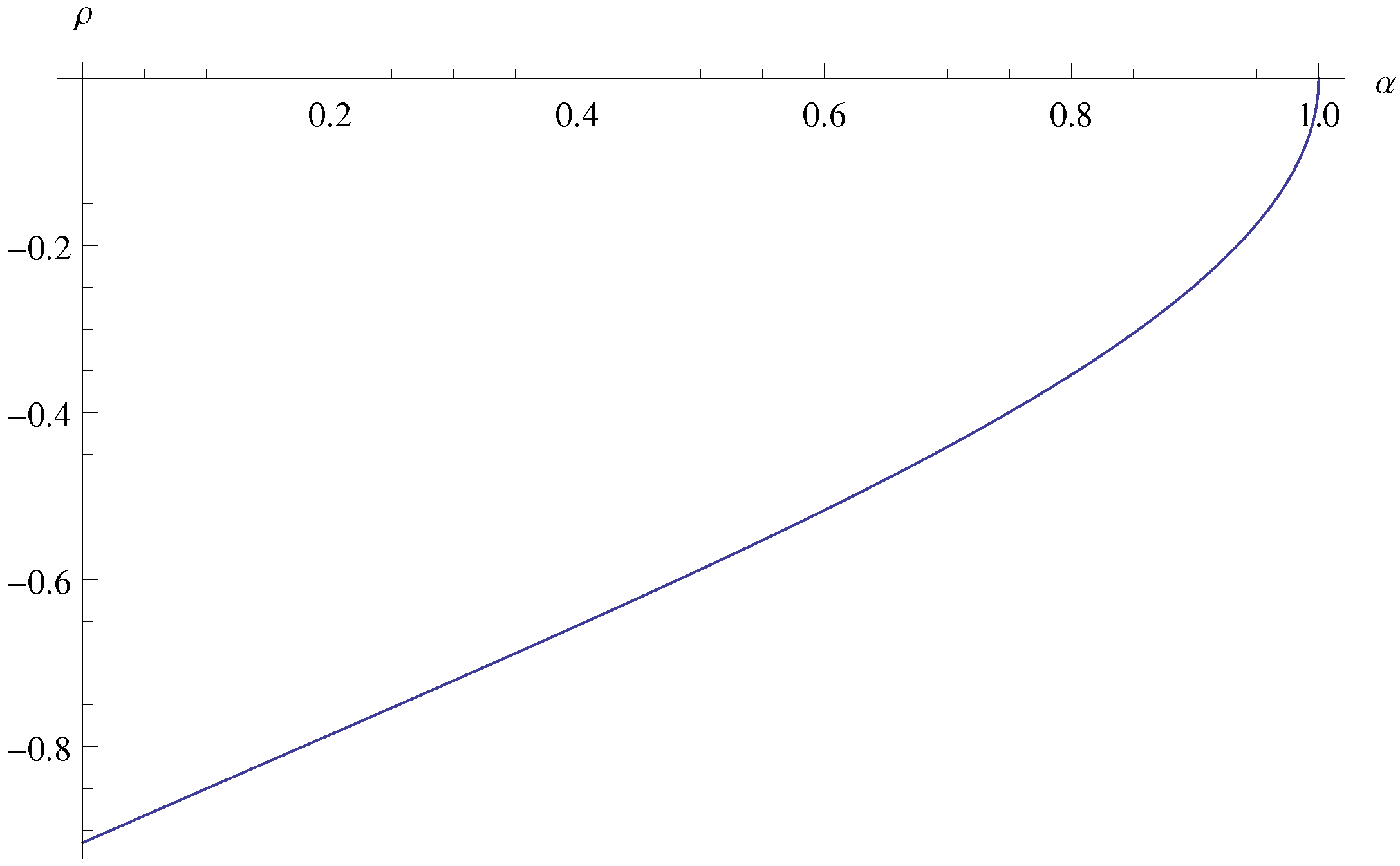
Determining $Var\left\{R_{(0)}^2\right\}$ by exploiting Equation (8) for $k=4$, we then arrive at the linear correlation coefficient

$$\rho (R_{(0)}^2,T_{\infty })=-\sqrt{\frac{3(\gamma -1)(3\gamma -1)(4\gamma -1)}{\gamma (43{\gamma }^2-7\gamma -6)}}.$$

Figure 1 depicts $\rho (R_{(0)}^2,T_{\infty })$ as a function of $\alpha =1/\gamma$. Note that ${lim}_{\gamma \to \infty }\rho (R_{(0)}^2,T_{\infty })=-6/\sqrt{43}$. The correlation coefficient allows to quantify the negative linear dependence between the two ratios (the dependence becomes weaker when α increases, as the maximum term will then typically be less dominant in the sum).

Figure 1. $\rho (R_{(0)}^2,T_{\infty })$ as a function of α.

Next, let us consider the case when the number of largest terms also increases as $t\to \infty$, but slower than the expected number of claims. It is now necessary to change the normalisation coefficients of $X_{N(t)-s}^{*}$ and ${\Sigma }_s(t)$.

Proposition 5. Let $s=⌊p(t)N(t)⌋\to \infty$ for a function $p(t)$ with $p(t)\to 0$ and $tp(t)\to \infty$. Then $\left({\Lambda }_s(t)/U(t),X_{N(t)-s}^{*}/U(p^{-1}(t)),{\Sigma }_s(t)/(tp(t)U(p^{-1}(t)))\right)\stackrel{D}{\to }(\Lambda ,\Xi ,\Sigma )$ where

$$E\left\{exp(-u\Lambda -v\Xi -w\Sigma )\right\}=e^{-v}{q}_0\left({\int }_0^{\infty }\frac{(1-e^{-u{z}^{-\gamma }\eta })}{{\eta }^{1+1/\gamma }}d\eta +\frac{w}{\gamma -1}\right).$$

(11)

If $\Theta =1$ a.s.

$$E\left\{exp(-u\Lambda -v\Xi -w\Sigma )\right\}=exp\left(-{\int }_0^{\infty }\frac{(1-e^{-u{z}^{-\gamma }\eta })}{{\eta }^{1+1/\gamma }}d\eta -v-\frac{w}{\gamma -1}\right).$$

Several messages may be derived from (11). First note that the asymptotic distribution of $X_{N(t)-s}^{*}$ is degenerated for $s=⌊p(t)N(t)⌋$, since $X_{N(t)-s}^{*}/U(p^{-1}(t))\stackrel{D}{\to }1$ as $t\to \infty$. Second, the asymptotic distribution of the sum of the smallest claims is the distribution of Θ up to a scaling factor, since ${\Sigma }_s(t)/(tp(t)U(p^{-1}(t)))\stackrel{D}{\to }\Theta /(\gamma -1)$ as $t\to \infty$.

Finally, for a fixed proportion of maximum terms, it is also necessary to change the normalisation coefficients of $X_{N(t)-s}^{*}$ and ${\Sigma }_s(t)$. We have

Proposition 6. Let $s=⌊pN(t)⌋$ for a fixed $0<p<1$. Then $\left({\Lambda }_s(t)/U(t),X_{N(t)-s}^{*},{\Sigma }_s(t)/t\right)\stackrel{D}{\to }({\Lambda }_p,{\Xi }_p,{\Sigma }_p)$ where

$$E\left\{exp(-u{\Lambda }_p-v{\Xi }_p-w{\Sigma }_p)\right\}=e^{-v{x}_p}{q}_0\left(u^{1/\gamma }\frac{\Gamma (1-1/\gamma )}{1-p}+wE\left\{X|X\le x_p\right\}\right)$$

and $x_p=F^{-1}(p)$. If $\Theta =1$ a.s.,

$$E\left\{exp(-u{\Lambda }_p-v{\Xi }_p-w{\Sigma }_p)\right\}=exp\left(-u^{1/\gamma }\frac{\Gamma (1-1/\gamma )}{1-p}-v{x}_p-wE\left\{X|X\le x_p\right\}\right).$$

As expected, $X_{N(t)-s}^{*}\stackrel{D}{\to }{x}_p$ and ${\Sigma }_s(t)/t\stackrel{D}{\to }\Theta E\left\{X|X\le x_p\right\}$ as $t\to \infty$. If $\Theta =1$ a.s. and $\gamma =2$, then ${\Lambda }_p$ has an inverse Gamma distribution with shape parameter equal to $1/2$.

4. Asymptotics for the Joint Laplace Transforms when $\gamma <1$

In this section, we assume that $\gamma <1$ and hence the expectation of the claim distribution is finite. We let $\mu =E\left\{X_1\right\}$. The normalisation coefficient of the sum of the smallest claims, ${\Sigma }_s(t)$, will therefore be $t^{-1}$ as it is the case for $S(t)$ for the Law of Large Numbers. In Section 5, we will then consider the sum of the smallest centered claims with another normalisation coefficient.

Again, consider a fixed s $\in \mathbb{N}$ first. The normalisation coefficients of ${\Lambda }_s(t)$ and $X_{N(t)-s}^{*}$ are the same as for the case $\gamma >1$, but the normalisation coefficient of ${\Sigma }_s$ is now $t^{-1}$.

Proposition 7. For fixed s $\in \mathbb{N}$, we have $\left({\Lambda }_s(t)/U(t),X_{N(t)-s}^{*}/U(t),{\Sigma }_s(t)/t\right)\stackrel{D}{\to }({\Lambda }_s,{\Xi }_s,{\Sigma }_s)$ where

$$E\left\{exp(-u{\Lambda }_s-v{\Xi }_s-w{\Sigma }_s)\right\}=\frac{1}{s!}{\int }_0^{\infty }{\left(\frac{z}{\gamma }{\int }_1^{\infty }\frac{e^{-u{z}^{-\gamma }\eta }}{{\eta }^{1+1/\gamma }}d\eta \right)}^s{e}^{-v{z}^{-\gamma }}{q}_{s+1}\left(z+w\mu \right)dz.$$

If $\Theta =1$ a.s.,

$$E\left\{exp(-u{\Lambda }_s-v{\Xi }_s-w{\Sigma }_s)\right\}=e^{-w\mu }\frac{1}{s!}{\int }_0^{\infty }{\left(\frac{z}{\gamma }{\int }_1^{\infty }\frac{e^{-u{z}^{-\gamma }\eta }}{{\eta }^{1+1/\gamma }}d\eta \right)}^s{e}^{-v{z}^{-\gamma }-z}dz.$$

Corollary 8. We have

$$E\left\{\frac{{\Sigma }_s}{{\Xi }_s}\right\}=\mu \frac{\Gamma (s-\gamma +1)}{s!}E\left\{{\Theta }^{1+\gamma }\right\}$$

and

$$E\left\{\frac{{\Xi }_0}{{\Lambda }_s+{\Xi }_s+{\Sigma }_s}\right\}=1-\mu {\int }_0^{\infty }{\int }_0^{\infty }{e}^{-u{z}^{-\gamma }}{q}_2\left(z+u\mu \right)dudz.$$

We first note that

$$E\left\{exp(-w{\Sigma }_s)\right\}=\frac{1}{s!}{\int }_0^{\infty }{z}^s{q}_{s+1}\left(z+w\mu \right)dz=E\left\{\frac{1}{s!}{\int }_0^{\infty }{z}^s(e^{-\left(z+w\mu \right)\Theta }{\Theta }^{s+1})dz\right\}=E\left\{e^{-w\mu \Theta }\right\}$$

and therefore ${\Sigma }_s(t)/t\stackrel{D}{\to }\mu \Theta$ as $t\to \infty$ for any fixed s $\in \mathbb{N}$. The influence of the largest claims on the sum becomes less and less important as t is large and is asymptotically negligible. This is very different from the case $\gamma >1$. In Theorem 1 in Downey and Wright [18], it is moreover shown that, as $n\to \infty$,

$$E\left\{\frac{X_n^{*}}{{\sum }_{j=1}^n{X}_j^{*}}\right\}=\frac{E\left\{X_n^{*}\right\}}{E\left\{{\sum }_{j=1}^n{X}_j^{*}\right\}}\left(1+o(1)\right).$$

This result is no more true in our framework when Θ is not degenerate at 1. Assume that $E\left\{{\Theta }^{\gamma }\right\}<\infty$. Using (3) and under a uniform integrability condition, one has

$$\underset{t\to \infty }{lim}E\left\{\frac{X_{N(t)}^{*}}{{\sum }_{j=1}^{N(t)}{X}_j^{*}}\right\}\frac{t}{U(t)}\ne \frac{{lim}_{t\to \infty }E\left\{X_{N(t)}^{*}\right\}/U(t)}{{lim}_{t\to \infty }E\left\{{\sum }_{j=1}^{N(t)}{X}_j^{*}\right\}/t}=\frac{\Gamma (1-\gamma )E\left\{{\Theta }^{\gamma }\right\}}{\mu E\left\{\Theta \right\}}.$$

Next, we consider the case with varying number of maximum terms. The normalisation coefficients of ${\Lambda }_s(t)$ and $X_{N(t)-s}^{*}$ now differ.

Proposition 9. Let $s=⌊p(t)N(t)⌋\to \infty$ and $p(t)\to 0$, i.e., $tp(t)\to \infty$. Then $\left({\Lambda }_s(t)/(tp(t)U(p^{-1}(t))),X_{N(t)-s}^{*}/U(p^{-1}(t)),{\Sigma }_s(t)/t\right)\stackrel{D}{\to }(\Lambda ,\Xi ,\Sigma )$ where

$$E\left\{exp(-u\Lambda -v\Xi -w\Sigma )\right\}=e^{-v}{q}_0\left(\frac{u}{1-\gamma }+w\mu \right).$$

If $\Theta =1$ a.s.,

$$E\left\{exp(-u\Lambda -v\Xi -w\Sigma )\right\}=e^{-u/(1-\gamma )}{e}^{-v}{e}^{-w\mu }.$$

As for the case $\gamma >1$, $X_{N(t)-s}^{*}/U(p^{-1}(t))\stackrel{P}{\to }1$ as $t\to \infty$. Moreover the asymptotic distribution of the sum of the largest claim is the distribution of Θ up to a scaling factor since ${\Lambda }_s(t)/(tp(t)U(p^{-1}(t)))\stackrel{D}{\to }\Theta /(1-\gamma )$ as $t\to \infty$. Finally note that ${\Sigma }_s(t)/t\stackrel{D}{\to }\mu \Theta$ as $t\to \infty$ as for the case when s was fixed.

Finally we fix p. Only the normalisation coefficient of ${\Lambda }_s(t)$ and its asymptotic distribution differ from the case $\gamma >1$.

Proposition 10. Let $s=⌊pN(t)⌋$ and $0<p<1$. Then $\left({\Lambda }_s(t)/t,X_{N(t)-s}^{*},{\Sigma }_s(t)/t\right)\stackrel{D}{\to }({\Lambda }_p,{\Xi }_p,{\Sigma }_p)$ where

$$E\left\{exp(-u{\Lambda }_p-v{\Xi }_p-w{\Sigma }_p)\right\}=e^{-v{x}_p}{q}_0\left(uE\left\{X|X>x_p\right\}+wE\left\{X|X\le x_p\right\}\right)$$

and $x_p=F^{-1}(p)$. If $\Theta =1$ a.s.,

$$E\left\{exp(-u{\Lambda }_p-v{\Xi }_p-w{\Sigma }_p)\right\}=e^{-uE\left\{X|X>x_p\right\}}{e}^{-v{x}_p}{e}^{-wE\left\{X|X\le x_p\right\}}.$$

We note that the normalisation of ${\Lambda }_s(t)$ is the same as for ${\Sigma }_s(t)$ and that ${\Lambda }_s(t)/t\stackrel{D}{\to }\Theta E\left\{X|X>x_p\right\}$ as $t\to \infty$.

5. Asymptotics for the Joint Laplace Transform for $\gamma <1$ with centered claims when s is fixed

In this section, we consider the sum of the smallest centered claims

$${\Sigma }_s^{(\mu )}(t)=\sum _{j=1}^{N(t)-s-1}\left(X_j^{*}-\mu \right)$$

instead of the sum of the smallest claims ${\Sigma }_s(t)$. Like for the Central Limit Theorem, we have to consider two sub-cases: $1/2<\gamma <1$ and $\gamma <1/2$.

For the sub-case $1/2<\gamma <1$, the normalisation coefficient of ${\Sigma }_s^{(\mu )}(t)$ is now $U^{-1}(t)$.

Proposition 11. For fixed s $\in \mathbb{N}$ and $1/2<\gamma <1$, we have

$$\left({\Lambda }_s(t)/U(t),X_{N(t)-s}^{*}/U(t),{\Sigma }_s^{(\mu )}(t)/U(t)\right)\stackrel{D}{\to }({\Lambda }_s,{\Xi }_s,{\Sigma }_s^{(\mu )}),$$

where

$$\begin{array}{cc}& E\left\{exp(-u{\Lambda }_s-v{\Xi }_s-w{\Sigma }_s^{(\mu )})\right\}\hfill \\ =& \frac{1}{s!}{\int }_0^{\infty }{\left(\frac{z}{\gamma }{\int }_1^{\infty }\frac{e^{-u{z}^{-\gamma }\eta }}{{\eta }^{1+1/\gamma }}d\eta \right)}^s{e}^{-v{z}^{-\gamma }}{q}_{s+1}\left(z\left(1+\frac{1}{\gamma }{\int }_0^1\frac{1-w{z}^{-\gamma }\eta -e^{-w{z}^{-\gamma }\eta }}{{\eta }^{1+1/\gamma }}d\eta -\frac{z^{-\gamma }}{1-\gamma }w\right)\right)dz.\hfill \end{array}$$

If $\Theta =1$ a.s.,

$$\begin{array}{ccc}& & E\left\{exp(-u{\Lambda }_s-v{\Xi }_s-w{\Sigma }_s^{(\mu )})\right\}\hfill \\ & =& \frac{1}{s!}{\int }_0^{\infty }{\left(\frac{z}{\gamma }{\int }_1^{\infty }\frac{e^{-u{z}^{-\gamma }\eta }}{{\eta }^{1+1/\gamma }}d\eta \right)}^s{e}^{-v{z}^{-\gamma }}exp\left(-z\left(1+\frac{1}{\gamma }{\int }_0^1\frac{1-w{z}^{-\gamma }\eta -e^{-w{z}^{-\gamma }\eta }}{{\eta }^{1+1/\gamma }}d\eta -\frac{z^{-\gamma }}{1-\gamma }w\right)\right)dz.\hfill \end{array}$$

If $s=0$, then

$$E\left\{exp(-v{\Xi }_0-w{\Sigma }_0^{(\mu )})\right\}={\int }_0^{\infty s}{e}^{-v{z}^{-\gamma }}exp\left(-z\left(1+\frac{1}{\gamma }{\int }_0^1\frac{1-w{z}^{-\gamma }\eta -e^{-w{z}^{-\gamma }\eta }}{{\eta }^{1+1/\gamma }}d\eta -\frac{z^{-\gamma }}{1-\gamma }w\right)\right)dz$$

and we see that ${\Xi }_0$ and ${\Sigma }_0^{(\mu )}$ are not independent.

Corollary 12. We have

$$E\left\{1+\frac{{\Sigma }_s^{(\mu )}}{{\Xi }_s}\right\}=1+\frac{s+1}{\gamma -1}.$$

This result is to compare with the one obtained by Bingham and Teugels [7] for $s=0$ (see also Ladoucette and Teugels [2]).

For the sub-case $\gamma <1/2$, let ${\sigma }^2=Var\left\{X_1\right\}$. The normalisation coefficient of ${\Sigma }_s^{(\mu )}(t)$ becomes $t^{-1/2}$.

Proposition 13. For s $\in \mathbb{N}$ fixed and $\gamma <1/2$, we have $\left({\Lambda }_s(t)/U(t),X_{N(t)-s}^{*}/U(t),{\Sigma }_s^{(\mu )}(t)/t^{1/2}\right)\stackrel{D}{\to }({\Lambda }_s,{\Xi }_s,{\Sigma }_s^{(\mu )})$ where

$$E\left\{exp(-u{\Lambda }_s-v{\Xi }_s-w{\Sigma }_s^{(\mu )})\right\}=\frac{1}{s!}{\int }_0^{\infty }{\left(\frac{z}{\gamma }{\int }_1^{\infty }\frac{e^{-u{z}^{-\gamma }\eta }}{{\eta }^{1+1/\gamma }}d\eta \right)}^s{e}^{-v{z}^{-\gamma }}{q}_{s+1}\left(z-\frac{1}{2}{w}^2{\sigma }^2\right)dz.$$

If $\Theta =1$ a.s.,

$$E\left\{exp(-u{\Lambda }_s-v{\Xi }_s-w{\Sigma }_s^{(\mu )})\right\}=\frac{1}{s!}exp\left(\frac{1}{2}{w}^2{\sigma }^2\right){\int }_0^{\infty }{\left(\frac{z}{\gamma }{\int }_1^{\infty }\frac{e^{-u{z}^{-\gamma }\eta }}{{\eta }^{1+1/\gamma }}d\eta \right)}^s{e}^{-v{z}^{-\gamma }-z}dz.$$

If $s=0$ and $\Theta =1$ a.s., we note that the maximum, ${\Xi }_0$, and the centred sum, ${\Sigma }_0^{(\mu )}$, are independent. If $s>0$ and $\Theta =1$ a.s., $\left({\Lambda }_s,{\Xi }_s\right)$ is independent of ${\Sigma }_s^{(\mu )}$.

6. Proofs

Proof of Proposition 3. In formula (7), we first use the substitution $\overline{F}(y)=z/t$, i.e., $y=U(t/z)$:

$$\begin{array}{cc}& {\Omega }_s(u/U(t),v/U(t),w/U(t))\hfill \\ =& \sum _{n=0}^s{p}_n(t){\left({\int }_0^{\infty }{e}^{-ux/U(t)}dF(x)\right)}^n\hfill \\ & +\frac{1}{s!}{\int }_0^t{\left({\int }_{U(t/z)}^{\infty }{e}^{-ux/U(t)}dF(x)\right)}^s{e}^{-vU(t/z)/U(t)}{Q}_t^{(s+1)}\left({\int }_0^{U(t/z)}{e}^{-wx/U(t)}dF(x)\right)\frac{dz}{t}\hfill \end{array}$$

$$\begin{array}{cc}=& \sum _{n=0}^s{p}_n(t){\left({\int }_0^{\infty }{e}^{-ux/U(t)}dF(x)\right)}^n\hfill \\ & +\frac{1}{s!}{\int }_0^t{\left(t{\int }_{U(t/z)}^{\infty }{e}^{-ux/U(t)}dF(x)\right)}^s{e}^{-vU(t/z)/U(t)}\hfill \\ & \times \frac{1}{t^{s+1}}{Q}_t^{(s+1)}\left(1-\frac{1}{t}\left(t-t{\int }_0^{U(t/z)}{e}^{-wx/U(t)}dF(x)\right)\right)dz.\hfill \end{array}$$

Next, the substitution $\overline{F}(x)=\rho z/t$, i.e., $x=U(t/(z\rho ))$ leads to

$$t{\int }_{U(t/z)}^{\infty }{e}^{-ux/U(t)}dF(x)=z{\int }_0^1{e}^{-uU(t/(z\rho ))/U(t)}d\rho \to z{\int }_0^1{e}^{-u{(z\rho )}^{-\gamma }}d\rho =\frac{z}{\gamma }{\int }_1^{\infty }\frac{e^{-u{z}^{-\gamma }\eta }}{{\eta }^{1+1/\gamma }}d\eta$$

as $t\to \infty$ and also

$$\begin{array}{c}\left(t-t{\int }_0^{U(t/z)}{e}^{-wx/U(t)}dF(x)\right)=t(1-F(U(t/z)))+t{\int }_0^{U(t/z)}(1-e^{-wx/U(t)})dF(x)\hfill \\ =z+z{\int }_1^{\infty }(1-e^{-wU(t/(z\rho ))/U(t)})d\rho \\ \hfill \to z\left(1+{\int }_1^{\infty }(1-e^{-w{(z\rho )}^{-\gamma }})d\rho \right)=z\left(1+\frac{1}{\gamma }{\int }_0^1\frac{1-e^{-w{z}^{-\gamma }\eta }}{{\eta }^{1+1/\gamma }}d\eta \right).\end{array}$$

Note that the integral is well defined since $\gamma >1$. Moreover $e^{-vU(t/z)/U(t)}\to e^{-v{z}^{-\gamma }}$ and

$$p_n(t){\left({\int }_0^{\infty }{e}^{-ux/U(t)}dF(x)\right)}^n\le p_n(t)\to 0\text{as}t\to \infty .$$

   ☐

Proof of Corollary 4. From Proposition 3 we have

$$E\left\{exp(-(u+v){\Xi }_s-u{\Sigma }_s)\right\}=\frac{1}{s!}{\int }_0^{\infty }{z}^s{e}^{-u{z}^{-\gamma }}{e}^{-v{z}^{-\gamma }}{q}_{s+1}\left(z\left(1+\frac{1}{\gamma }{\int }_0^1\frac{1-e^{-u{z}^{-\gamma }\eta }}{{\eta }^{1+1/\gamma }}d\eta \right)\right)dz.$$

Hence

$$\begin{array}{ccc}\hfill {\left.\frac{\partial }{\partial u}E\left\{exp(-(u+v){\Xi }_s-u{\Sigma }_s)\right\}\right|}_{u=0}& =& -\frac{1}{s!}{\int }_0^{\infty }{z}^s{z}^{-\gamma }{e}^{-v{z}^{-\gamma }}{q}_{s+1}\left(z\right)dz\hfill \\ & & -\frac{1}{s!\left(\gamma -1\right)}{\int }_0^{\infty }{z}^{s+1}{z}^{-\gamma }{e}^{-v{z}^{-\gamma }}{q}_{s+2}\left(z\right)dz.\hfill \end{array}$$

This gives indeed, using (3),

$$\begin{array}{c}E\left\{\frac{{\Xi }_s+{\Sigma }_s}{{\Xi }_s}\right\}=-{\int }_0^{\infty }{\left.\frac{\partial }{\partial u}E\left\{exp(-(u+v){\Xi }_s-u{\Sigma }_s)\right\}\right|}_{u=0}dv\hfill \\ \hfill =\frac{1}{s!}{\int }_0^{\infty }{z}^s{q}_{s+1}\left(z\right)dz+\frac{1}{s!\left(\gamma -1\right)}{\int }_0^{\infty }{z}^{s+1}{q}_{s+2}\left(z\right)dz=1+\frac{s+1}{\gamma -1}\end{array}$$

which extends (5) to the case of NMP processes. Next, we focus on (8) for general k. We first consider the case $s=0$. We have

$$E\left\{{\left(1+\frac{{\Sigma }_0}{{\Xi }_0}\right)}^k\right\}=\sum _{i=0}^k\left(\begin{array}{c}k\\ i\end{array}\right)E\left\{{\left(\frac{{\Sigma }_0}{{\Xi }_0}\right)}^i\right\}.$$

Let

$$\theta (z,w)=z\left(1+\frac{1}{\gamma }{\int }_0^1\frac{1-e^{-w{z}^{-\gamma }\eta }}{{\eta }^{1+1/\gamma }}d\eta \right).$$

By Proposition 3

$$E\left\{exp(-v{\Xi }_0-w{\Sigma }_0)\right\}={\int }_0^{\infty }{e}^{-v{z}^{-\gamma }}{q}_1\left(\theta (z,w)\right)dz$$

(12)

and clearly

$$E\left\{{\left(\frac{{\Sigma }_0}{{\Xi }_0}\right)}^i\right\}=\frac{{(-1)}^i}{\Gamma (i)}{\int }_0^{\infty }{v}^{i-1}{\left.\frac{{\partial }^i}{\partial w^i}E(exp(-v{\Xi }_0-w{\Sigma }_0))\right|}_{w=0}dv.$$

Note that

$$\begin{array}{ccc}\hfill {\theta }^{\left(1\right)}(z,w):=& & \frac{\partial }{\partial w}\theta (z,w)=\frac{z^{-\gamma +1}}{\gamma }{\int }_0^1{\eta }^{-1/\gamma }{e}^{-w{z}^{-\gamma }\eta }d\eta \hfill \\ \hfill {\theta }^{\left(n\right)}(z,w):=& & \frac{{\partial }^n}{\partial w^n}\theta (z,w)={\left(-1\right)}^{n+1}\frac{z^{-n\gamma +1}}{\gamma }{\int }_0^1{\eta }^{-1/\gamma +(n-1)}{e}^{-w{z}^{-\gamma }\eta }d\eta ,\hfill \end{array}$$

so

$${\theta }^{\left(n\right)}(z,0)={\left(-1\right)}^{n+1}{z}^{-n\gamma +1}\frac{1}{n\gamma -1}.$$

By the Faa di Bruno’s formula

$$\frac{{\partial }^n}{\partial w^n}{q}_1\left(\theta (z,w)\right)=\sum _{k=0}^n{q}_1^{(k)}\left(\theta (z,w)\right)B_{n,k}\left({\theta }^{\left(1\right)}(z,w),\dots ,{\theta }^{\left(n-k+1\right)}(z,w)\right)$$

where

$$B_{n,k}\left(x_1,\dots ,x_{n-k+1}\right)=\sum _{\begin{array}{c}{m}_1+\dots +m_{n-k+1}=k\\ 1m_1+2m_2+\dots +(n-k+1)m_{n-k+1}=n\end{array}}\frac{n!}{m_1!m_2!\dots m_{n-k+1}!}\prod _{j=1}^{n-k+1}{\left(\frac{x_j}{j!}\right)}^{m_j}.$$

Therefore

$${\left.\frac{{\partial }^n}{\partial w^n}{q}_1\left(\theta (z,w)\right)\right|}_{w=0}=\sum _{k=1}^n{\left(-1\right)}^k{q}_{k+1}\left(z\right)B_{n,k}\left(\frac{z^{-\gamma +1}}{\gamma -1},\dots ,{\left(-1\right)}^{n-k}\frac{z^{-(n-k+1)\gamma +1}}{(n-k+1)\gamma -1}\right).$$

Subsequently,

$$\begin{array}{ccc}& & B_{n,k}\left(\frac{z^{-\gamma +1}}{\gamma -1},\dots ,{\left(-1\right)}^{n-k}\frac{z^{-(n-k+1)\gamma +1}}{(n-k+1)\gamma -1}\right)\hfill \\ & =& \sum _{\begin{array}{c}{m}_1+\dots +m_{n-k+1}=k\\ 1m_1+2m_2+\dots +(n-k+1)m_{n-k+1}=n\end{array}}\frac{n!}{m_1!m_2!\dots m_{n-k+1}!}\prod _{j=1}^{n-k+1}{\left(\frac{{\left(-1\right)}^{j+1}}{j!}{z}^{-j\gamma +1}\frac{1}{j\gamma -1}\right)}^{m_j}\hfill \\ & =& z^{-n\gamma +k}{\left(-1\right)}^{n+k}\sum _{\begin{array}{c}{m}_1+\dots +m_{n-k+1}=k\\ 1m_1+2m_2+\dots +(n-k+1)m_{n-k+1}=n\end{array}}\frac{n!}{m_1!m_2!\dots m_{n-k+1}!}\prod _{j=1}^{n-k+1}{\left(\frac{1}{j!\left(j\gamma -1\right)}\right)}^{m_j}\hfill \\ & =& z^{-n\gamma +k}{\left(-1\right)}^{n+k}{C}_{n,k}\left(\gamma \right)\hfill \end{array}$$

with definition (9). This gives

$${\left.\frac{{\partial }^n}{\partial w^n}{q}_1\left(\theta (z,w)\right)\right|}_{w=0}=z^{-n\gamma +k}{\left(-1\right)}^n\sum _{k=1}^n{q}_{k+1}\left(z\right)C_{n,k}\left(\gamma \right)$$

and

$${\left.\frac{{\partial }^i}{\partial w^i}E(exp(-v{\Xi }_0-w{\Sigma }_0))\right|}_{w=0}={\int }_0^{\infty }{e}^{-v{z}^{-\gamma }}\left(z^{-i\gamma +k}{\left(-1\right)}^i\sum _{k=1}^i{q}_{k+1}\left(z\right)C_{i,k}\left(\gamma \right)\right)dz,$$

so that

$$\begin{array}{ccc}\hfill E\left\{{\left(\frac{{\Sigma }_0}{{\Xi }_0}\right)}^i\right\}& =& \frac{1}{\Gamma (i)}{\int }_0^{\infty }{v}^{i-1}\left[{\int }_0^{\infty }{e}^{-v{z}^{-\gamma }}\left(z^{-i\gamma +k}\sum _{k=1}^i{q}_{k+1}\left(z\right)C_{i,k}\left(\gamma \right)\right)dz\right]dv\hfill \\ & =& \frac{1}{\Gamma (i)}\sum _{k=1}^i{C}_{i,k}\left(\gamma \right){\int }_0^{\infty }{q}_{k+1}\left(z\right)z^{-i\gamma +k}\left[{\int }_0^{\infty }{v}^{i-1}{e}^{-v{z}^{-\gamma }}dv\right]dz\hfill \\ & =& \frac{1}{\Gamma (i)}\sum _{k=1}^i{C}_{i,k}\left(\gamma \right){\int }_0^{\infty }{q}_{k+1}\left(z\right)z^{-i\gamma +k}\frac{\Gamma (i)}{{\left(z^{-\gamma }\right)}^i}dz\hfill \\ & =& \sum _{k=1}^i{C}_{i,k}\left(\gamma \right){\int }_0^{\infty }{q}_{k+1}\left(z\right)z^{k}dz\hfill \\ & =& \sum _{k=1}^{i}k!C_{i,k}\left(\gamma \right)\hfill \end{array}$$

cf. (3), and the result follows.

For the case $s>0$, we proceed in an analogous way. Equation (12) becomes

$$E\left\{exp(-v{\Xi }_s-w{\Sigma }_s)\right\}={\int }_0^{\infty }{z}^s{e}^{-v{z}^{-\gamma }}{q}_{s+1}\left(\theta (z,w)\right)dz.$$

Then ${\Sigma }_0/{\Xi }_0$ is replaced by ${\Sigma }_s/{\Xi }_s$, $q_1\left(z\right)$ by $q_{s+1}\left(z\right)$, $q_1^{(k)}$ by $q_{s+1}^{(k)}$ and, by following the same path as for $s=0$, we get

$$E\left\{{\left(\frac{{\Sigma }_s}{{\Xi }_s}\right)}^i\right\}=\sum _{k=1}^i{C}_{i,k}\left(\gamma \right){\int }_0^{\infty }{q}_{s+k+1}\left(z\right)z^{s+k}dz=\sum _{k=1}^i\frac{(s+k)!}{s!}{C}_{i,k}\left(\gamma \right).$$

   ☐

Proof of Proposition 5. The proof is similar to the previous one, so we just highlight the differences here: Conditioning on $N(t)=n$ we have

$$\begin{array}{ccc}& & E_{N(t)=n}\left\{exp(-u{\Lambda }_s(t)/U(t)-v{X}_{n(1-p(t))}^{*}/U(p^{-1}(t)))-w{\Sigma }_s(t))/(tp(t)U(p^{-1}(t)))\right\}\hfill \\ & =& \frac{n!}{(np(t))!(n(1-p(t)))!}{\int }_0^{\infty }{\left({\int }_y^{\infty }{e}^{-ux/U(t)}dF(x)\right)}^{np(t)}{e}^{-vy/U(p^{-1}(t))}\hfill \\ & & \times {\left({\int }_0^y{e}^{-wx/(tp(t)U(p^{-1}(t)))}dF(x)\right)}^{n(1-p(t))-1}dF(y).\hfill \end{array}$$

We first replace F by the substitution $\overline{F}(y)=p(t)z$, i.e., $y=U(1/(p(t)z))$:

$$\begin{array}{ccc}& & {\left.{\Omega }_s(u/U(t),v/U(p^{-1}(t)),w/(tp(t)U(p^{-1}(t)));t)\right|}_{N(t)=n}\hfill \\ & =& \frac{n!}{(np(t))!(n(1-p(t)))!}{\int }_0^{\infty }{\left({\int }_{U(1/(p(t)z))}^{\infty }{e}^{-ux/(tp(t)U(p^{-1}(t))}dF(x)\right)}^{np(t)}{e}^{-vU(1/(p(t)z))/U(p^{-1}(t))}\hfill \\ & & \times {\left({\int }_0^{U(1/(p(t)z))}{e}^{-wx/(tp(t)U(p^{-1}(t)))}dF(x)\right)}^{n(1-p(t))-1}p(t)dz\hfill \end{array}$$

The factor involving v converges to

$$e^{-vU(1/(p(t)z))/U(p^{-1}(t))}\to e^{-v{z}^{-\gamma }}.$$

The factor containing w behaves as

$$\begin{array}{ccc}\hfill {\int }_0^{U(1/(p(t)z))}{e}^{-wx/(tp(t)U(p^{-1}(t)))}dF(x)& =& 1-p(t)z-{\int }_0^{U(1/(p(t)z))}(1-e^{-wx/(tp(t)U(p^{-1}(t)))}dF(x)\hfill \\ & =& 1-p(t)z-w{\int }_0^{U(1/(p(t)z))}\frac{x}{(tp(t)U(p^{-1}(t)))}dF(x)+\dots \hfill \\ & =& 1-p(t)z-w\frac{r\left(U(1/(p(t)z))\right)}{(tp(t)U(p^{-1}(t)))}+\dots \hfill \\ & =& 1-p(t)z-\frac{w}{t}\frac{z^{1-\gamma }}{\gamma -1}+\dots \hfill \end{array}$$

and hence for the power

$$\begin{array}{c}{\left({\int }_0^{U(1/(p(t)z))}{e}^{-wx/(tp(t)U(p^{-1}(t)))}dF(x)\right)}^{n(1-p(t))-1}\hfill \\ =exp\left(n(1-p(t))ln\left(1-p(t)z-\frac{w}{t}\frac{z^{1-\gamma }}{\gamma -1}+\dots \right)\right)\\ \hfill =exp\left(np(t)z-\frac{n}{t}w\frac{z^{1-\gamma }}{\gamma -1}-np(t)ln\left(1-p(t)z+\dots \right)\right).\end{array}$$

Finally, for the factor containing u, replace F by the substitution $\overline{F}(x)=\rho z/t$, i.e., $x=U(t/(z\rho ))$:

$$\begin{array}{ccc}\hfill {\int }_{U(1/(p(t)z))}^{\infty }{e}^{-ux/U(t)}dF(x)& \sim & \frac{z}{t}{\int }_0^{tp(t)}{e}^{-uU(t/(z\rho ))/U(t)}d\rho \hfill \\ & \sim & \frac{z}{t}{\int }_0^{tp(t)}\left(e^{-uU(t/(z\rho ))/U(t)}-1\right)d\rho +p(t)z\hfill \\ & \sim & p(t)z\left(1-\frac{1}{tp(t)}{\int }_0^{\infty }(1-e^{-u{(z\rho )}^{-\gamma }})d\rho \right)\hfill \\ & \sim & p(t)z\left(1-\frac{1}{tp(t)}{\int }_0^{\infty }\frac{(1-e^{-u{z}^{-\gamma }\eta })}{{\eta }^{1+1/\gamma }}d\eta \right)\hfill \end{array}$$

so that, as $t\to \infty$,

$$\begin{array}{c}{\left({\int }_{U(1/(p(t)z))}^{\infty }{e}^{-ux/(tp(t)U(p^{-1}(t))}dF(x)\right)}^{np(t)}\hfill \\ \hfill \sim exp\left(np(t)lnz+np(t)lnp(t)-\frac{n}{t}{\int }_0^{\infty }\frac{(1-e^{-u{z}^{-\gamma }\eta })}{{\eta }^{1+1/\gamma }}d\eta \right).\end{array}$$

For the factor with the factorials, we have by Stirling’s formula

$$\frac{n!}{np(t)!(n(1-p(t))-1)!}\sim \frac{1}{\sqrt{2\pi }}\frac{n^{1/2}}{e^{(np(t)+1/2)ln(p(t))}{e}^{(n(1-p(t))+1/2)ln(1-p(t)}}.$$

(13)

Equivalent for the integral in z:

$$\begin{array}{ccc}\hfill g(z)& =& ln(z)-z\hfill \\ \hfill g^{\prime }(z)& =& \frac{1}{z}-1g^{\prime }(1)=0\hfill \\ \hfill g^{″}(z)& =& -\frac{1}{z^2}{g}^{″}(1)=-1\hfill \end{array}$$

By Laplace’s method, we deduce that

$${\int }_0^{\infty }exp\left(np(t)(ln(z)-z)\right)dz\sim \frac{\sqrt{2\pi }}{n^{1/2}{p}^{1/2}(t)}exp\left(-np(t)\right).$$

(14)

Altogether

$$\begin{array}{ccc}& & {\left.{\Omega }_s(u/U(t),v/U(p^{-1}(t)),w/(tp(t)U(p^{-1}(t))))\right|}_{N(t)=n}\hfill \\ & \sim & e^{-v}exp\left(-\frac{n}{t}w\frac{1}{\gamma -1}+o\left(\frac{n}{t}\right)+np(t)ln\left(1-p(t)\right)+np(t)lnp(t)\right)\hfill \\ & & \times exp\left(-\frac{n}{t}{\int }_0^{\infty }\frac{(1-e^{-u{z}^{-\gamma }\eta })}{{\eta }^{1+1/\gamma }}d\eta -np(t)lnp(t)-np(t)-\frac{1}{2}ln(p(t))+ln(p(t))\right)\hfill \\ & & \times exp\left(-(np(t)+1/2)ln(p(t))-(n(1-p(t))+1/2)ln(1-p(t)\right)\hfill \\ & \sim & exp\left(-\frac{n}{t}{\int }_0^{\infty }\frac{(1-e^{-u{z}^{-\gamma }\eta })}{{\eta }^{1+1/\gamma }}d\eta -v-\frac{n}{t}w\frac{1}{\gamma -1}\right).\hfill \end{array}$$

   ☐

Proof of Proposition 6. Again, we condition on $N(t)=n$:

$$\begin{array}{ccc}& & E_{N(t)=n}\left\{exp(-u{\Lambda }_s(t)/U(t)-v{X}_{n(1-p)}^{*}-w{\Sigma }_s(t))/t\right\}\hfill \\ & =& \frac{n!}{np!(n(1-p)-1)!}{\int }_0^{\infty }{\left({\int }_y^{\infty }{e}^{-ux/U(t)}dF(x)\right)}^{np}{e}^{-vy}{\left({\int }_0^y{e}^{-wx/t}dF(x)\right)}^{n(1-p)-1}dF(y).\hfill \end{array}$$

For the factor containing w, we have

$$\begin{array}{ccc}\hfill {\int }_0^y{e}^{-wx/t}dF(x)& =& P(X\le y)-\frac{w}{t}{\int }_0^{y}xdF(x)+o(t^{-1})\hfill \\ & =& P(X\le y)\left(1-\frac{w}{t}E\left\{X|X\le y\right\}+o(t^{-1})\right)\hfill \\ & =& F(y)\left(1-\frac{w}{t}E\left\{X|X\le y\right\}+o(t^{-1})\right).\hfill \end{array}$$

For the factor involving u one can write

$$\begin{array}{ccc}\hfill {\int }_y^{\infty }{e}^{-ux/U(t)}dF(x)& =& -{\left[e^{-ux/U(t)}\overline{F}(x)\right]}_y^{\infty }-{\int }_y^{\infty }{e}^{-ux/U(t)}\frac{x}{U(t)}\overline{F}(x)dx\hfill \\ & =& e^{-uy/U(t)}\overline{F}(y)-{\int }_{uy/U(t)}^{\infty }{e}^{-w}\overline{F}\left(\frac{w}{u}U(t)\right)dw\hfill \\ & =& \overline{F}(y)-\frac{1}{t}{u}^{1/\gamma }{\int }_0^{\infty }{e}^{-w}{w}^{-1/\gamma }dw\left(1+o(1)\right)\hfill \\ & =& \overline{F}(y)-\frac{1}{t}{u}^{1/\gamma }\Gamma (1-1/\gamma )\left(1+o(1)\right).\hfill \end{array}$$

The ratio with factorials behaves, by Stirling’s formula, as

$$\begin{array}{ccc}\hfill \frac{n!}{np!(n(1-p)-1)!}& \sim & \frac{\sqrt{2\pi }{n}^{n+1/2}{e}^{-n}}{\sqrt{2\pi }{(np)}^{np+1/2}{e}^{-np}\sqrt{2\pi }{(n(1-p))}^{n(1-p)+1/2}{e}^{-np}}\hfill \\ & \sim & \frac{1}{\sqrt{2\pi }}\frac{n^{1/2}}{p^{np+1/2}{(1-p)}^{n(1-p)+1/2}}.\hfill \end{array}$$

For the integral in y we have the equivalence

$$\begin{array}{ccc}& & {\left({\int }_y^{\infty }{e}^{-ux/t}dF(x)\right)}^{np}{\left({\int }_0^y{e}^{-wx/t}dF(x)\right)}^{n(1-p)-1}\hfill \\ & =& exp\left(n\left(pln(F(y)+(1-p)ln(\overline{F}(y))\right)\right)exp\left(-w\frac{n}{t}pE\left\{X|X\le y\right\}-u\frac{n}{t}E\left\{X|X>y\right\}\right).\hfill \end{array}$$

Let

$$\begin{array}{ccc}\hfill g(y)& =& pln(F(y))+(1-p)ln(\overline{F}(y))\hfill \\ \hfill g^{\prime }(y)& =& p\frac{f(y)}{F(y)}-(1-p)\frac{f(y)}{\overline{F}(y)}\hfill \\ \hfill F(y_p)& =& p,y_p=F^{-1}(p)\hfill \\ \hfill g(y_p)& =& pln(p)+(1-p)ln(1-p)\hfill \\ \hfill g^{″}(y)& =& p\frac{f^{\prime }(y)F(y)-f^2(y)}{F^2(y)}-(1-p)\frac{f^{\prime }(y)\overline{F}(y)+f^2(y)}{{\overline{F}}^2(y)}\hfill \\ \hfill g^{″}(y_p)& =& f^{\prime }(y_p)-\frac{f^2(y_p)}{p}-f^{\prime }(y_p)-\frac{f^2(y_p)}{1-p}=-\frac{f^2(y_p)}{p(1-p)}.\hfill \end{array}$$

By Laplace’s method, we deduce that

$$exp\left(n\left(pln(F(y)+(1-p)ln(\overline{F}(y))\right)\right)\sim \frac{\sqrt{2\pi }\sqrt{p(1-p)}}{n^{1/2}}{e}^{n\left(pln(p)+(1-p)ln(1-p)\right)}$$

and then

$$\begin{array}{ccc}& & {\int }_0^{\infty }{\left({\int }_y^{\infty }{e}^{-ux/t}dF(x)\right)}^{np}{e}^{-vy}{\left({\int }_0^y{e}^{-wx/t}dF(x)\right)}^{n(1-p)-1}dF(y)\hfill \\ & \sim & \frac{\sqrt{2\pi }\sqrt{p(1-p)}}{n^{1/2}}{e}^{n\left(pln(p)+(1-p)ln(1-p)\right)}exp\left(-u\Theta E\left\{X|X>y_p\right\}-v{y}_p-w\Theta pE\left\{X|X\le y_p\right\}\right).\hfill \end{array}$$

Altogether

$${\Omega }_s(u/t,v,w/t;t)\to e^{-v{y}_p}{q}_0\left(uE\left\{X|X>y_p\right\}+wE\left\{X|X\le y_p\right\}\right).$$

   ☐

Proof of Proposition 7. We first replace F by the substitution $\overline{F}(y)=z/t$, i.e., $y=U(t/z)$

$$\begin{array}{c}{\Omega }_s(u/U(t),v/U(t),w/t;t)=\sum _{n=0}^s{p}_n(t){\left({\int }_0^{\infty }{e}^{-ux/U(t)}dF(x)\right)}^s\hfill \\ \hfill +\frac{1}{s!}{\int }_0^t{\left(t{\int }_{U(t/z)}^{\infty }{e}^{-ux/U(t)}dF(x)\right)}^s{e}^{-vU(t/z)/U(t)}\frac{1}{t^{s+1}}{Q}_t^{(s+1)}\left({\int }_0^{U(t/z)}{e}^{-wx/t}dF(x)\right)dz.\end{array}$$

Then we have

$$\begin{array}{ccc}\hfill {\int }_0^{U(t/z)}{e}^{-wx/t}dF(x)& =& F(U(t/z))-\frac{w}{t}{\int }_0^{U(t/z)}xdF(x)+o\left(\frac{1}{t}\right)\hfill \\ & =& 1-\frac{z}{t}-\frac{w}{t}\mu +o\left(\frac{1}{t}\right)=1-\frac{1}{t}\left(z+w\mu +o\left(1\right)\right).\hfill \end{array}$$

Now use analogous arguments as in the proof of Proposition 3 and note that

$$\begin{array}{ccc}\hfill E\left\{exp(-uS(t)/t)\right\}& =& Q_t\left(E\left\{exp(-uX/t)\right\}\right)=Q_t\left({\int }_0^{\infty }{e}^{-ux/t}dF(x)\right)\hfill \\ & =& Q_t\left(1-\frac{u}{t}{\int }_0^{\infty }xdF(x)+o\left(\frac{1}{t}\right)\right)\hfill \\ & \to & q_0\left(u\mu \right).\hfill \end{array}$$

   ☐

Proof of Corollary 8. By Proposition 7

$$E\left\{exp(-v{\Xi }_s-u{\Sigma }_s)\right\}=\frac{1}{s!}{\int }_0^{\infty }{z}^s{e}^{-v{z}^{-\gamma }}{q}_{s+1}\left(z+u\mu \right)dz.$$

Hence

$${\left.\frac{\partial }{\partial u}E\left\{exp(-v{\Xi }_s-u{\Sigma }_s)\right\}\right|}_{u=0}=-\frac{\mu }{s!}{\int }_0^{\infty }{z}^s{e}^{-v{z}^{-\gamma }}{q}_{s+2}\left(z\right)dz$$

and therefore

$$\begin{array}{ccc}\hfill -{\int }_0^{\infty }{\left.\frac{\partial }{\partial u}E\left\{exp(-(u+v){\Xi }_s-u{\Sigma }_s)\right\}\right|}_{u=0}dv& =& \frac{\mu }{s!}{\int }_0^{\infty }{z}^{s-\gamma }{q}_{s+2}\left(z\right)dz\hfill \\ & =& \mu \frac{\Gamma (s-\gamma +1)}{s!}E\left\{{\Theta }^{1+\gamma }\right\}.\hfill \end{array}$$

By Proposition 7

$$E\left\{exp(-(u+v){\Xi }_0-u{\Sigma }_0)\right\}={\int }_0^{\infty }{e}^{-(u+v)z^{-\gamma }}{q}_1\left(z+u\mu \right)dz$$

$${\left.\frac{\partial }{\partial v}E\left\{exp(-(u+v){\Xi }_0-u{\Sigma }_0)\right\}\right|}_{v=0}=-{\int }_0^{\infty }{z}^{-\gamma }{e}^{-u{z}^{-\gamma }}{q}_1\left(z+u\mu \right)dz$$

$$\begin{array}{ccc}& & -{\int }_0^{\infty }{\left.\frac{\partial }{\partial v}E\left\{exp(-(u+v){\Xi }_0-u{\Sigma }_0)\right\}\right|}_{v=0}du\hfill \\ & =& {\int }_0^{\infty }{\int }_0^{\infty }{z}^{-\gamma }{e}^{-u{z}^{-\gamma }}{q}_1\left(z+u\mu \right)dudz\hfill \\ & =& {\int }_0^{\infty }\left(-{\left[e^{-u{z}^{-\gamma }}{q}_1\left(z+u\mu \right)\right]}_0^{\infty }-\mu {\int }_0^{\infty }{e}^{-u{z}^{-\gamma }}{q}_2\left(z+u\mu \right)du\right)dz\hfill \\ & =& {\int }_0^{\infty }{q}_1\left(z\right)dz-\mu {\int }_0^{\infty }{\int }_0^{\infty }{e}^{-u{z}^{-\gamma }}{q}_2\left(z+u\mu \right)dudz\hfill \\ & =& 1-\mu {\int }_0^{\infty }{\int }_0^{\infty }{e}^{-u{z}^{-\gamma }}{q}_2\left(z+u\mu \right)dudz.\hfill \end{array}$$

   ☐

Proof of Proposition 9. Condition on $N(t)=n$ to see that

$$\begin{array}{ccc}& & E_{N(t)=n}\left\{exp(-u{\Lambda }_s(t)/(tp(t)U(p^{-1}(t)))-v{X}_{n(1-p(t))}^{*}/U(p^{-1}(t)))-w{\Sigma }_s(t))/t\right\}\hfill \\ & =& \frac{n!}{np(t)!(n(1-p(t)))!}{\int }_0^{\infty }{\left({\int }_y^{\infty }{e}^{-ux/(tp(t)U(p^{-1}(t))}dF(x)\right)}^{np(t)}{e}^{-vy/U(p^{-1}(t))}\hfill \\ & & \times {\left({\int }_0^y{e}^{-wx/t}dF(x)\right)}^{n(1-p(t))-1}dF(y).\hfill \end{array}$$

Now replace F by the substitution $\overline{F}(y)=p(t)z$, i.e., $y=U(1/(p(t)z))$

$$\begin{array}{cc}& {\Omega }_s(u/(tp(t)U(p^{-1}(t))),v/U(p^{-1}(t)),w/t;t)\hfill \\ =& \frac{n!}{np(t)!(n(1-p(t)))!}{\int }_0^{\infty }{\left({\int }_{U(1/(p(t)z))}^{\infty }{e}^{-ux/(tp(t)U(p^{-1}(t))}dF(x)\right)}^{np(t)}\hfill \\ & \times e^{-vU(1/(p(t)z))/U(p^{-1}(t))}{\left({\int }_0^{U(1/(p(t)z))}{e}^{-wx/t}dF(x)\right)}^{n(1-p(t))-1}p(t)dz.\hfill \end{array}$$

Like before,

$$e^{-vU(1/(p(t)z))/U(p^{-1}(t))}\to e^{-v{z}^{-\gamma }}.$$

For the factor with w, one sees that

$$\begin{array}{ccc}\hfill {\int }_0^{U(1/(p(t)z))}{e}^{-wx/t}dF(x)& =& F(U(1/(p(t)z)))-\frac{w}{t}{\int }_0^{U(1/(p(t)z))}xdF(x)+o\left(\frac{1}{t}\right)...\hfill \\ & =& 1-p(t)z-\frac{w}{t}\mu +o\left(\frac{1}{t}\right)...\hfill \end{array}$$

and then

$$\begin{array}{ccc}\hfill {\left({\int }_0^{U(1/(p(t)z))}{e}^{-wx/t}dF(x)\right)}^{n(1-p(t))-1}& =& exp\left(n(1-p(t))ln\left(1-p(t)z-\frac{w}{t}\mu +o\left(\frac{1}{t}\right)\right)\right)\hfill \\ & =& exp\left(-np(t)z-\frac{n}{t}w\mu +o\left(\frac{n}{t}\right)+np(t)ln\left(1-p(t)z\right)\right).\hfill \end{array}$$

For the factor with u, replace F by the substitution $\overline{F}(x)=p(t)\rho z$, i.e., $x=U(1/(p(t)z\rho ))$:

$$t{\int }_{U(t/z)}^{\infty }{e}^{-ux/U(t)}dF(x)=z{\int }_0^1{e}^{-uU(t/(z\rho ))/U(t)}d\rho \to z{\int }_0^1{e}^{-u{(z\rho )}^{-\gamma }}d\rho =\frac{z}{\gamma }{\int }_1^{\infty }\frac{e^{-u{z}^{-\gamma }\eta }}{{\eta }^{1+1/\gamma }}d\eta$$

$$\begin{array}{ccc}\hfill {\int }_{U(1/(p(t)z))}^{\infty }{e}^{-ux/(tp(t)U(p^{-1}(t))}dF(x)& =& p(t)z{\int }_0^1{e}^{-uU(p^{-1}(t)/(z\rho ))/U(p^{-1}(t))tp(t)}d\rho \hfill \\ & =& p(t)z\left(1-\frac{1}{tp(t)}{\int }_0^{1}u{(z\rho )}^{-\gamma }d\rho +\right)\hfill \\ & =& p(t)z\left(1-\frac{1}{1-\gamma }\frac{z^{-\gamma }}{tp(t)}u{\int }_0^1{\rho }^{-\gamma }d\rho +\dots \right)\hfill \end{array}$$

and then

$$\begin{array}{ccc}& & {\left({\int }_{U(1/(p(t)z))}^{\infty }{e}^{-ux/(tp(t)U(p^{-1}(t))}dF(x)\right)}^{np(t)}\hfill \\ & =& exp\left(np(t)lnp(t)+np(t)ln(z)-\frac{n}{t}\frac{u}{1-\gamma }{z}^{-\gamma }+\dots \right).\hfill \end{array}$$

The ratio of factorials coincides with (13). Also (14) applies here. Altogether

$$\begin{array}{cc}& \frac{n!}{np(t)!(n(1-p(t)))!}{\int }_0^{\infty }{\left({\int }_{U(1/(p(t)z))}^{\infty }{e}^{-ux/(tp(t)U(p^{-1}(t))}dF(x)\right)}^{np(t)}{e}^{-vU(1/(p(t)z))/U(p^{-1}(t))}\hfill \\ & \times {\left({\int }_0^{U(1/(p(t)z))}{e}^{-wx/t}dF(x)\right)}^{n(1-p(t))-1}p(t)dz\hfill \\ \sim & e^{-v}exp\left(-\frac{n}{t}w\mu +o\left(\frac{n}{t}\right)+np(t)ln\left(1-p(t)\right)+np(t)lnp(t)-\frac{n}{t}\frac{u}{1-\gamma }-np(t)-\frac{1}{2}lnp(t)+lnp(t)\right)\hfill \\ & \times exp\left(-(np(t)+1/2)lnp(t)-(n(1-p(t))+1/2)ln(1-p(t)\right)\hfill \\ \sim & exp\left(-\frac{n}{t}\frac{u}{1-\gamma }-v-\frac{n}{t}w\mu \right).\hfill \end{array}$$

   ☐

Proof of Proposition 10. Given $N(t)=n$

$$\begin{array}{ccc}& & E_{N(t)=n}\left\{exp(-u{\Lambda }_s(t)/t-v{X}_{n(1-p)}^{*}-w{\Sigma }_s(t))/t\right\}\hfill \\ & =& \frac{n!}{np!(n(1-p)-1)!}{\int }_0^{\infty }{\left({\int }_y^{\infty }{e}^{-ux/t}dF(x)\right)}^{np}{e}^{-vy}{\left({\int }_0^y{e}^{-wx/t}dF(x)\right)}^{n(1-p)-1}dF(y).\hfill \end{array}$$

The part involving w coincides with the one in the proof of Proposition 6. For the factor involving u, we have

$$\begin{array}{ccc}\hfill {\int }_y^{\infty }{e}^{-ux/t}dF(x)& =& P(X>y)-\frac{u}{t}{\int }_y^{\infty }xdF(x)+o(t^{-1})\hfill \\ & =& \overline{F}(y)\left(1-\frac{u}{t}E\left\{X|X>y\right\}+o(t^{-1})\right).\hfill \end{array}$$

The rest of the proof is completely analogous to the one for Proposition 6.     ☐

Proof of Proposition 11. Use the substitution $\overline{F}(y)=z/t$, i.e., $y=U(t/z)$:

$$\begin{array}{cc}& {\Omega }_s^{(\mu )}(u{\Lambda }_s(t)/U(t),v{X}_{N(t)-s}^{*}/U(t),w{\Sigma }_s^{(\mu )}(t)/U(t);t)\hfill \\ =& \sum _{n=0}^s{p}_n(t){\left({\int }_0^{\infty }{e}^{-ux/U(t)}dF(x)\right)}^s\hfill \\ & +\frac{1}{s!}{\int }_0^t{\left(t{\int }_{U(t/z)}^{\infty }{e}^{-ux/U(t)}dF(x)\right)}^s{e}^{-vU(t/z)/U(t)}\hfill \\ & \times \frac{1}{t^{s+1}}{Q}_t^{(s+1)}\left(1-\frac{1}{t}\left(t-t{e}^{w\mu /U(t)}{\int }_0^{U(t/z)}{e}^{-wx/U(t)}dF(x)\right)\right)dz.\hfill \end{array}$$

We then replace F by the substitution $\overline{F}(x)=\rho z/t$, i.e., $x=U(t/(z\rho ))$:

$$\begin{array}{ccc}& & t-t{e}^{w\mu /U(t)}{\int }_0^{U(t/z)}{e}^{-wx/U(t)}dF(x)\hfill \\ & =& t+t{e}^{w\mu /U(t)}{\int }_0^{U(t/z)}\left(1-\frac{wx}{U(t)}-e^{-wx/U(t)}\right)dF(x)-t{e}^{w\mu /U(t)}F(U(t/z))\hfill \\ & & +t{e}^{w\mu /U(t)}{\int }_0^{U(t/z)}\frac{wx}{U(t)}dF(x)\hfill \\ & =& t\left(1-e^{w\mu /U(t)}\left(1-\frac{z}{t}\right)\right)+z{\int }_1^{\infty }\left(1-w\frac{U(t/(z\rho ))}{U(t)}-e^{-wU(t/(z\rho ))/U(t)}\right)d\rho \hfill \\ & & +\frac{tw}{U(t)}{e}^{w\mu /U(t)}\left(\mu -\frac{z^{1-\gamma }}{1-\gamma }\frac{U(t)}{t}(1+o(1))\right)\hfill \\ & =& t\left(1-\left(1+\frac{w\mu }{U(t)}+\frac{1}{2}{\left(\frac{w\mu }{U(t)}\right)}^2+o\left(\frac{1}{U^2(t)}\right)\right)\left(1-\frac{z}{t}\right)\right)\hfill \\ & & +z{\int }_1^{\infty }\left(1-w\frac{U(t/(z\rho ))}{U(t)}-e^{-wU(t/(z\rho ))/U(t)}\right)d\rho +\frac{tw\mu }{U(t)}\left(1+\frac{w\mu }{U(t)}+o\left(\frac{1}{U(t)}\right)\right)\left(1+O(1/t)\right)\hfill \end{array}$$

$$\begin{array}{ccc}& =& z+z{\int }_1^{\infty }\left(1-w\frac{U(t/(z\rho ))}{U(t)}-e^{-wU(t/(z\rho ))/U(t)}\right)d\rho -\frac{z^{1-\gamma }}{1-\gamma }w+O\left(\frac{1}{U(t)}\right)+O\left(\frac{t}{U^2(t)}\right)\hfill \\ & \to & z\left(1+{\int }_1^{\infty }(1-w{(z\rho )}^{-\gamma }-e^{-w{(z\rho )}^{-\gamma }})d\rho -\frac{z^{-\gamma }}{1-\gamma }w\right)\hfill \\ & =& z\left(1+\frac{1}{\gamma }{\int }_0^1\frac{1-w{z}^{-\gamma }v-e^{-w{z}^{-\gamma }\eta }}{{\eta }^{1+1/\gamma }}d\eta -\frac{z^{-\gamma }}{1-\gamma }w\right).\hfill \end{array}$$

Now use the same arguments as in the proof of Proposition     ☐

Proof of Corollary 12. Note that

$$\begin{array}{cc}& E\left\{exp(-(u+v){\Xi }_s-u{\Sigma }_s^{(\mu )})\right\}\hfill \\ =& \frac{1}{s!}{\int }_0^{\infty }{z}^s{e}^{-v{z}^{-\gamma }}{e}^{-u{z}^{-\gamma }}{q}_{s+1}\left(z\left(1+\frac{1}{\gamma }{\int }_0^1\frac{1-u{z}^{-\gamma }v-e^{-u{z}^{-\gamma }\eta }}{{\eta }^{1+1/\gamma }}d\eta -\frac{z^{-\gamma }}{1-\gamma }u\right)\right)dz\hfill \end{array}$$

$$\begin{array}{cc}& {\left.\frac{\partial }{\partial u}E\left\{exp(-(u+v){\Xi }_s-u{\Sigma }_s)\right\}\right|}_{u=0}\hfill \\ =& -\frac{1}{s!}{\int }_0^{\infty }{z}^s{z}^{-\gamma }{e}^{-v{z}^{-\gamma }}{q}_{s+1}\left(z\right)dz+\frac{1}{\left(1-\gamma \right)s!}{\int }_0^{\infty }{z}^{1+s}{z}^{-\gamma }{e}^{-v{z}^{-\gamma }}{q}_{s+2}\left(z\right)dz\hfill \\ & \hspace{1em}-{\int }_0^{\infty }{\left.\frac{\partial }{\partial u}E\left\{exp(-(u+v){\Xi }_s-u{\Sigma }_s^{(\mu )})\right\}\right|}_{u=0}dv=1+\frac{s+1}{\gamma -1}.\hfill \end{array}$$

   ☐

Proof of Proposition 13. Use the substitution $\overline{F}(y)=z/t$, i.e., $y=U(t/z)$:

$$\begin{array}{cc}& {\Omega }_s^{(\mu )}(u{\Lambda }_s(t)/U(t),v{X}_{N(t)-s}^{*}/U(t),w{\Sigma }_s^{(\mu )}/t^{1/2};t)\hfill \\ =& \sum _{n=0}^s{p}_n(t){\left({\int }_0^{\infty }{e}^{-ux/U(t)}dF(x)\right)}^s\hfill \\ & +\frac{1}{s!}{\int }_0^t{\left(t{\int }_{U(t/z)}^{\infty }{e}^{-ux/U(t)}dF(x)\right)}^s{e}^{-vU(t/z)/U(t)}\hfill \\ & \times \frac{1}{t^{s+1}}{Q}_t^{(s+1)}\left(1-\frac{1}{t}\left(t-t{e}^{w\mu /t^{1/2}}{\int }_0^{U(t/z)}{e}^{-wx/t^{1/2}}dF(x)\right)\right)dz.\hfill \end{array}$$

Then we have

$$\begin{array}{cc}& t-t{e}^{w\mu /t^{1/2}}{\int }_0^{U(t/z)}{e}^{-wx/t^{1/2}}dF(x)\hfill \\ =& t+t{e}^{w\mu /t^{1/2}}{\int }_0^{U(t/z)}\left(1-\frac{wx}{t^{1/2}}+\frac{1}{2}\frac{{\left(wx\right)}^2}{t}-e^{-wx/t^{1/2}}\right)dF(x)-t{e}^{w\mu /t^{1/2}}F(U(t/z))\hfill \\ & +t{e}^{w\mu /t^{1/2}}{\int }_0^{U(t/z)}\frac{wx}{t^{1/2}}dF(x)-\frac{1}{2}{e}^{w\mu /t^{1/2}}{\int }_0^{U(t/z)}{\left(wx\right)}^{2}dF(x).\hfill \end{array}$$

First note that

$$\begin{array}{ccc}& & t{e}^{w\mu /t^{1/2}}{\int }_0^{U(t/z)}\left(1-\frac{wx}{t^{1/2}}+\frac{1}{2}\frac{{\left(wx\right)}^2}{t}-e^{-wx/t^{1/2}}\right)dF(x)\hfill \\ & =& z{e}^{w\mu /t^{1/2}}{\int }_1^{\infty }\left(1-w\frac{U(t/(z\rho ))}{t^{1/2}}+\frac{1}{2}{\left(w\frac{U(t/(z\rho ))}{t^{1/2}}\right)}^2-e^{-wU(t/(z\rho ))/t^{1/2}}\right)d\rho \to 0.\hfill \end{array}$$

Secondly,

$$\begin{array}{cc}& t-t{e}^{w\mu /t^{1/2}}F(U(t/z))+t{e}^{w\mu /t^{1/2}}{\int }_0^{U(t/z)}\frac{wx}{t^{1/2}}dF(x)-\frac{1}{2}{e}^{w\mu /t^{1/2}}{\int }_0^{U(t/z)}{\left(wx\right)}^{2}dF(x)\hfill \\ =& t\left(1-e^{w\mu /t^{1/2}}\left(1-\frac{z}{t}\right)\right)+\frac{tw}{t^{1/2}}{e}^{w\mu /t^{1/2}}\left(\mu -U(t/z)\frac{z}{t}-{\int }_{U(t/z)}^{\infty }\overline{F}(x)dx\right)\hfill \\ & -\frac{1}{2}{e}^{w\mu /t^{1/2}}\left(E\left\{X_1^2\right\}-{\int }_{U(t/z)}^{\infty }{x}^{2}dF(x)\right)\hfill \\ =& t\left(1-e^{w\mu /t^{1/2}}\left(1-\frac{z}{t}\right)\right)+\frac{tw}{t^{1/2}}{e}^{w\mu /t^{1/2}}\left(\mu -\frac{1}{1-\gamma }U(t/z)\frac{z}{t}(1+o(1))\right)\hfill \\ =& -\frac{1}{2}{w}^2{e}^{w\mu /t^{1/2}}\left(E\left\{X_1^2\right\}-\gamma {\left(U(t/z)\right)}^2\frac{z}{t}(1+o(1)\right)\hfill \\ =& t\left(1-\left(1+\frac{w\mu }{t^{1/2}}+\frac{1}{2}{\left(\frac{w\mu }{t^{1/2}}\right)}^2+o\left(\frac{1}{t}\right)\right)\left(1-\frac{z}{t}\right)\right)\hfill \\ & +t^{1/2}\mu w\left(1+\frac{w\mu }{t^{1/2}}+\frac{1}{2}{\left(\frac{w\mu }{t^{1/2}}\right)}^2+o\left(\frac{1}{t}\right)\right)\left(1-\frac{1}{\mu (1-\gamma )}U(t/z)\frac{z}{t}(1+o(1)\right)\hfill \\ & -\frac{1}{2}{w}^2\left(1+\frac{w\mu }{t^{1/2}}+\frac{1}{2}{\left(\frac{w\mu }{t^{1/2}}\right)}^2+o\left(\frac{1}{t}\right)\right)\left(E\left\{X_1^2\right\}-\gamma {\left(U(t/z)\right)}^2\frac{z}{t}(1+o(1)\right)\hfill \end{array}$$

and it follows that

$$\begin{array}{ccc}& & t-t{e}^{w\mu /t^{1/2}}F(U(t/z))+t{e}^{w\mu /t^{1/2}}{\int }_0^{U(t/z)}\frac{wx}{t^{1/2}}dF(x)-\frac{1}{2}{e}^{w\mu /t^{1/2}}{\int }_0^{U(t/z)}{\left(wx\right)}^{2}dF(x)\hfill \\ & =& z-t^{1/2}\mu w-\frac{1}{2}{\left(w\mu \right)}^2+o(1)+t^{1/2}\mu w+{\left(w\mu \right)}^2+O\left(\frac{U(t)}{t^{1/2}}\right)-\frac{1}{2}{w}^{2}E\left\{X_1^2\right\}+O\left({\left(\frac{U(t)}{t^{1/2}}\right)}^2\right)\hfill \\ & \to & z-\frac{1}{2}{w}^2{\sigma }^2,\hfill \end{array}$$

which completes the proof. Note that

$$\begin{array}{ccc}\hfill E\left\{exp(-u(S(t)-N(t)\mu )/t^{1/2})\right\}& =& Q_t\left(E\left\{exp(-u(X-\mu )/t^{1/2})\right\}\right)\hfill \\ & =& Q_t\left({\int }_0^{\infty }{e}^{-u(x-\mu )/t^{1/2}}dF(x)\right)\hfill \\ & =& Q_t\left(1+\frac{u^2}{2t}{\sigma }^2+o\left(\frac{1}{t}\right)\right).\hfill \\ & \to & q_0\left(-\frac{u^2}{2}{\sigma }^2\right)=E\left\{e^{u^2{\sigma }^2\Theta /2}\right\}.\hfill \end{array}$$

   ☐

7. Conclusions

In this paper we provided a fairly general collection of results on the joint asymptotic Laplace transforms of the normalised sums of smallest and largest among regularly varying claims, when the length of the considered time interval tends to infinity. This extends several classical results in the field. The appropriate scaling of the different quantities is essential. We showed to what extent the type of the near mixed Poisson process counting the number of claim instances influences the limit results, and also identified quantities for which this influence is asymptotically negligible. We further related the dominance of the maximum term in such a random sum to another quantity that exhibits the effect of the tail index on the aggregate claim rather explicitly, namely the ratio of sum of squares of the claims over the sum of the claims squared. The results allow to further quantify the effect of large claims on the total claim amount in an insurance portfolio, and could hence be helpful in the design of appropriate reinsurance programs when facing heavy-tailed claims with regularly varying tail. Particular emphasis is given to the case when the tail index exceeds 1, which corresponds to infinite-mean claims, a situation that is particularly relevant for catastrophe modelling.