Model Risk in Portfolio Optimization

Abstract

We consider a one-period portfolio optimization problem under model uncertainty. For this purpose, we introduce a measure of model risk. We derive analytical results for this measure of model risk in the mean-variance problem assuming we have observations drawn from a normal variance mixture model. This model allows for heavy tails, tail dependence and leptokurtosis of marginals. The results show that mean-variance optimization is seriously compromised by model uncertainty, in particular, for non-Gaussian data and small sample sizes. To mitigate these shortcomings, we propose a method to adjust the sample covariance matrix in order to reduce model risk.

1. Introduction

Traditional portfolio optimization techniques rely on the true model parameters being known. However, in general, these model parameters are not known and need to be estimated, for example, from historical data. The possible estimation error gives rise to model risk or model uncertainty. Let us illustrate this with a prominent example, the mean-variance optimization introduced by Markowitz [1]. Consider the unconstrained version of the optimization problem

$$\mathrm{maximize}({\mathit{\mu }}^{\prime }\mathit{w}-\kappa {\mathit{w}}^{\prime }\Sigma \mathit{w})\mathrm{over}\mathit{w}\in {\mathbb{R}}^n$$

where $\mathit{\mu }\in {\mathbb{R}}^n$ is the vector of expected returns, $\Sigma \in {\mathbb{R}}^{n\times n}$ is the positive definite covariance matrix and $\kappa >0$ is a risk aversion parameter. This optimization problem has a unique solution ${\mathit{w}}^{*}\in {\mathbb{R}}^n$ given by

$${\mathit{w}}^{*}=\frac{1}{2\kappa }{\Sigma }^{-1}\mathit{\mu }$$

This solution crucially depends on the true expected returns μ and the covariance matrix Σ. The standard approach replaces true parameters by estimates ignoring any model uncertainty. In the literature, it has been shown that this standard approach has serious drawbacks in mean-variance optimization, see e.g., Michaud [2].

The aim of this paper is to study analytically and numerically the consequences of such model uncertainty in the mean-variance problem and derive parameter estimators which take model uncertainty into account. Despite being a standard one-period problem, it becomes mathematically rather involved when considering model uncertainty. We remark that the mean-variance portfolio remains one of the most important benchmarks in the literature on asset allocation and in the asset management industry, see e.g., Litterman, [3] Chapter 4, and Meucci, [4] Chapter 6. Numerically we will also analyze three other important benchmarks in asset allocation: the minimum variance, the equal contributions to risk and the maximum diversification problems; see e.g., Choueifaty and Coignard [5], Maillard et al. [6] and Clarke et al. [7] for more information about the latter problems. In this paper we consider these four major portfolio optimization problems. There is an extensive literature discussing mean-variance optimization under model uncertainty. We briefly review the main contributions.

A first portfolio selection rule which takes model uncertainty into account has initially been studied in Brown [8,9], and Klein and Bawa [10]. They use a Bayesian approach under a non-informative prior. In this framework, the optimal portfolio is selected maximizing the expected value of the objective function conditioned on the predictive distribution of the asset returns. This approach mostly outperforms the standard one and has been studied in many subsequent articles, see e.g., Kandel and Stambaugh [11], Barberis [12], Pástor [13], Pástor and Stambaugh [14], Xia [15], and Tu and Zhou [16].

A second approach to deal with model uncertainty has been proposed in Jobson et al. [17], Jorion [18], and Frost and Savarino [19]. This consists in adjusting the estimated parameters in order to minimize or reduce a certain loss function. The loss function measures the negative effects of model uncertainty. Typically, it is defined by the expected loss in the mean-variance objective function caused by the estimation. In [17,18,19] the mean-variance problem is considered within the Bayesian framework using such a loss function. This approach differs from the one in [9] and subsequent papers. In [17,18,19] informative priors are proposed with the aim of exploiting prior knowledge about the problem and reducing estimation bias and error for the optimal portfolio weights. In [17] Stein-type estimators (also known as shrinkage estimators) for μ and Σ are introduced. In [18] the problem is studied under uncertainty in μ only. In [19] the mean-variance problem with linear constraints is considered under uncertainty in both μ and Σ. Ter Horst et al. [20] analyze the same loss function as in [17,18,19] under the assumption of known covariance matrix Σ and considering only estimation of μ. A uniform rescaling of the optimal portfolio weights is proposed to account for model uncertainty. In Kan and Zhou [21] a closed-form expression for the same loss function as in [17,18,19] is derived in the unconstrained mean-variance problem under uncertainty in μ and Σ. In Jobson and Korkie [22] the asymptotic distributions of the means, variances and optimal portfolio weights are derived in a constrained problem. Mori [23] obtains analytical results on the optimality of certain estimators in the constrained mean-variance problem. General linear equality constraints are considered under uncertainty in μ and Σ. Unlike these papers we use a more general class of models for the data than the multivariate Gaussian assumption. Moreover, we consider a modification of the loss function used in [17,18,19].

As mentioned above, other optimization problems than mean-variance are also used in practice. In particular, many variants involving different optimization criteria and different notions of risk have been proposed. For this reason an appropriate model risk measure should be defined for a relatively general portfolio optimization problem. In Kondor et al. [24] model uncertainty in a risk minimization problem is studied under several different risk measures using simulated data. The loss function considered in [24] is essentially a generalization of the one used in [17,18,19] to other risk measures than the variance. In this paper we introduce a measure of model risk in a more general portfolio optimization context than mean-variance or risk minimization.

Finally, Simaan [25] introduced an alternative loss measure to [17,18,19] based on the opportunity cost of forgoing the optimal portfolio. The opportunity cost is defined by the minimal amount of money the investor is willing to accept to replace the optimal portfolio with an alternative sub-optimal portfolio. If the investor has full information on the true parameters, then the amount is positive. However, under model uncertainty, the alternative portfolio may be superior out-of-sample and the amount may be negative. In the framework of [25] the opportunity cost is evaluated and used to study the effects of model uncertainty on the portfolio optimization. This approach is fundamentally different from the one we follow in this paper.

Ledoit and Wolf [26], partially motivated by portfolio optimization applications, propose a shrinkage estimator for Σ defined by the convex linear combination of the sample covariance matrix and the identity matrix. The optimal weight in the combination is determined asymptotically for number of assets and observations going simultaneously to infinity, i.e., they obtain asymptotically optimal covariance estimators. An alternative portfolio selection rule to the shrinkage of the sample covariance matrix is considered in DeMiguel et al. [27]. The approach of [27] can be interpreted as a shrinkage procedure for the optimal portfolio weights. This is achieved by imposing an additional constraint on the norm of the weights in the optimization. The paper shows that this corresponds to a Bayesian approach where the investor has prior information on the optimal portfolio weights rather than the means and the covariances. Recently, Zhou et al. [28] have considered an estimator based on a different regularization structure. Monotonicity constraints on the covariances and a smoothness penalty term are imposed when estimating the covariance matrix. They argue that a monotonic structure for the covariance matrix is common in several situations, e.g., bonds with different maturities and options with different strikes or expirations. In [28] the use of these smooth monotonic estimators is also extended to non-Gaussian data. In contrast, in our paper we do not attempt to reduce estimation error based on prior information about the structure of the problem; rather, we define a measure which describes how estimation uncertainty affects portfolio optimization. We study the properties of this measure under non-Gaussian data, and modify the estimates accordingly.

El Karoui [29,30] derives asymptotic results which highlight the severe problems arising in high-dimensional optimization problems. The minimum variance problem with linear constraints and uncertainty in μ and Σ is considered under elliptical asset returns. The considerations in our paper are in the spirit of [29,30] but relate to finite number of assets and sample size.

To conclude the review of the literature we would like to mention the deterministic approach studied in Goldfarb and Iyengar [31]. In this framework model parameters are known to lie within appropriately defined bounded sets. The optimization problem is then solved assuming worst case scenarios in these sets. In [31] an efficient algorithm to compute such robust optimal portfolios is developed.

In this paper we give the following contributions. First, we introduce a measure of model risk based on an alternative loss function to the one initially proposed by Jobson et al. [17], Jorion [18], and Frost and Savarino [19]. In Section 2 we introduce this measure in a general optimization problem and describe the reason why we believe it is more relevant for applications than the one considered in [17,18,19].

Secondly, most of the articles so far, have quantified model risk assuming $\mathrm{i}.\mathrm{i}.\mathrm{d}.$ multivariate Gaussian observations. This is, of course, not a realistic model for asset returns in the financial market, see e.g., McNeil et al. [32], Chapter 3. In Ter Horst et al. [20] a non-$\mathrm{i}.\mathrm{i}.\mathrm{d}.$ case is considered. In [29,30] non-$\mathrm{i}.\mathrm{i}.\mathrm{d}.$ elliptical data is considered and the problem is analyzed asymptotically. In this paper we derive analytical results for finite number of assets and observations in a normal variance mixture model which allows for heavy tails, tail dependence and leptokurtosis of marginals. In particular, we study the cases of small and large number of assets relative to the sample size. Note also that some articles in the literature (see e.g., [20]) consider only uncertainty in μ. From the analytical results derived in Kan and Zhou [21], it follows that the uncertainty in the covariance matrix also has a large impact on the optimal portfolio when the number of assets is large compared to the sample size. Therefore, in this paper, we consider uncertainty in both μ and Σ.

Finally, we present an alternative method to adjust the estimated parameters for model uncertainty. We consider modifications of the spectral decomposition of the sample covariance matrix in order to reduce the drawbacks of model risk. In the literature, we can find many papers studying the spectrum of the sample covariance matrix statistically, see e.g., Johnstone [33], Ledoit and Wolf [26], and El Karoui [34]. It has been shown that, although the sample covariance matrix is an unbiased estimator, its eigenvalues behave very differently from the true ones, especially, when the number of assets is large compared to the sample size. The linear shrinkage procedure of Ledoit and Wolf [26] corresponds to shrinking all the eigenvalues towards the same constant. In Ledoit and Wolf [35], it is argued that this approach works well in the case where the true eigenvalues are close to each other (this is typically the case when the number of assets is small compared to the sample size). However, if the eigenvalues are highly dispersed (typically the case when the number of assets is large compared to the sample size) linear shrinkage does not substantially improve the estimation. In their work they propose to apply an individual shrinkage to each sample eigenvalue in order to obtain an improvement in the covariance matrix estimation. This, however, without a direct consideration to portfolio optimization. The procedure to estimate the shrinkage intensities for each eigenvalue is based on a large dimensional asymptotic approximation, which relies on results from random matrix theory on the limiting spectral distribution of the sample covariance matrix, see Marchenko and Pastur [36]. Papp et al. [37] investigate a filtering procedure for the sample covariance matrix. Specifically, they consider a result which provides an exact relationship between the spectral moments of the true matrix and the sample ones. This can be used to revise the spectrum of the sample estimator. The applicability of this procedure is demonstrated using simulated data. In Menchero et al. [38] we find an empirical study on the bias of volatility estimates for mean-variance portfolios and its relations to eigenvalues and eigenvectors of the sample covariance matrix. In this paper we revisit the idea of modifying the eigenvalues individually and apply it to reduce the negative effects of model uncertainty. In particular, we analyze the measure of model uncertainty introduced in Section 2 in the mean-variance problem for the covariance matrix estimator with rescaled eigenvalues.

Organization of the paper. In Section 2 we introduce our measure of model risk for general portfolio optimization problems. Using this measure we prove in Proposition 1 the following result: under the assumption of known constraints and unbiased estimators, optimal portfolios are on average negatively affected by model risk. In Section 3 we consider mean-variance optimization assuming we have observations drawn from a normal variance mixture model. We derive in Theorem 2 an analytical formula for our measure of model uncertainty. This provides a good description of the effects of model uncertainty. Moreover, we show that this measure of model risk attains its lowest value in the Gaussian case. In Section 4 we introduce an estimator for the covariance matrix with adjusted eigenvalues. In Theorem 4 we derive a relationship between our measure of model uncertainty and the adjusted eigenvalues. Using this, we derive in Theorem 5 a rule which reduces the effects of model uncertainty under the assumption of known eigenvectors. Even if these are unknown, we show numerically in Section 5 that the rule provides significant improvements to the portfolio optimization problem.

2. General Definitions

We consider the portfolio optimization problem of an investor who allocates his wealth among n risky assets. A portfolio is defined by $\mathit{w}={(w_1,\dots ,w_n)}^{\prime }\in {\mathbb{R}}^n$, where $w_i$ denotes the proportion of wealth invested in asset i. Let $U:{\mathbb{R}}^n\to \mathbb{R}$ be a real-valued function on the set of all portfolios. The function U specifies the investor’s preference for portfolios and is called utility function. Let $\mathcal{A}\subset {\mathbb{R}}^n$ be the set of admissible portfolios which specifies the investment constraints. In this general setting we define the optimal portfolio by

$${\mathit{w}}^{*}(U,\mathcal{A})={\mathrm{argmax}}_{\mathit{w}\in \mathcal{A}}U\left(\mathit{w}\right)$$

(1)

under the assumption that the maximization problem has a unique solution. We think of ${\mathit{w}}^{*}(U,\mathcal{A})\in {\mathbb{R}}^n$ as the optimal portfolio based on utility U and constraints specified by $\mathcal{A}$. In Example 1 we give prominent examples of the general optimization problem (1).

Example 1. 

Assume the investor has complete knowledge of the mean vector $\mathit{\mu }\in {\mathbb{R}}^n$ and the covariance matrix $\Sigma \in {\mathbb{R}}^{n\times n}$ of the asset returns. We assume Σ is positive definite and formulate four major portfolio optimization problems. For a detailed description of the first two problems we refer to Meucci [4], Chapter 6.3–6.5. For the latter two see Choueifaty and Coignard [5], Maillard et al. [6], and Clarke et al. [7].

(i)

Mean-variance optimization: the investor is assumed to maximize

$$U^{\mathrm{mv}}\left(\mathit{w}\right)={\mathit{\mu }}^{\prime }w-\kappa {\mathit{w}}^{\prime }\Sigma \mathit{w}$$

where $\kappa >0$ is a given risk aversion parameter. The solution of Equation (1) in the unconstrained case can be calculated using first order conditions and is given by

$${\mathit{w}}^{*}(U^{\mathrm{mv}},{\mathbb{R}}^n)=\frac{1}{2\kappa }{\Sigma }^{-1}\mathit{\mu }$$

In the case of linear constraints we set $\mathcal{A}=\{\mathit{w}\in {\mathbb{R}}^n|A^{\prime }\mathit{w}=\mathbb{a}\}$, where $A\in {\mathbb{R}}^{n\times k}$ is a matrix of rank k and $\mathit{a}\in {\mathbb{R}}^k$. The solution of Equation (1) can be calculated using the method of Lagrange and is given by

$${\mathit{w}}^{*}(U^{\mathrm{mv}},\mathcal{A})=\frac{1}{2\kappa }\left({\Sigma }^{-1}-{\Sigma }^{-1}A{\left(A^{\prime }{\Sigma }^{-1}A\right)}^{-1}{A}^{\prime }{\Sigma }^{-1}\right)\mathit{\mu }+{\Sigma }^{-1}A{\left(A^{\prime }{\Sigma }^{-1}A\right)}^{-1}\mathit{a}$$

(ii)

Minimum variance: the investor is assumed to maximize the following utility function

$$U^{\mathrm{v}}\left(\mathit{w}\right)=-{\mathit{w}}^{\prime }\Sigma \mathit{w}$$

Consider the following linear equality constraints $\mathcal{A}=\{\mathit{w}\in {\mathbb{R}}^n|A^{\prime }\mathit{w}=\mathit{a}\mathrm{and}{\mathit{w}}^{\prime }\mathit{\mu }={\mu }_0\}$, where $A\in {\mathbb{R}}^{n\times k}$ is a matrix of rank k, $\mathit{a}\in {\mathbb{R}}^k$ and ${\mu }_0\in \mathbb{R}$. In this problem we are looking for the portfolio with minimal variance satisfying linear constraints and having expected return equal to ${\mu }_0$. The optimal portfolio can be calculated using the method of Lagrange and is given by

$${\mathit{w}}^{*}(U^{\mathrm{v}},\mathcal{A})={\Sigma }^{-1}\tilde{A}{\left({\tilde{A}}^{\prime }{\Sigma }^{-1}\tilde{A}\right)}^{-1}\tilde{\mathit{a}}$$

where $\tilde{A}=(A,\mathit{\mu })\in {\mathbb{R}}^{n\times (k+1)}$ and $\tilde{\mathit{a}}={({\mathit{a}}^{\prime },{\mathit{\mu }}_0)}^{\prime }\in {\mathbb{R}}^{k+1}$. In this example note that the set of admissible strategies $\mathcal{A}$ also depends on the distribution of the random returns through the mean vector μ.

(iii)

Equal contributions to risk: the investor is assumed to maximize

$$U^{\mathrm{ecr}}\left(\mathit{w}\right)=-\sum _{\begin{array}{c}i,j=1,\dots ,n\\ i<j\end{array}}{\left({\mathrm{RC}}_i\left(\mathit{w}\right)-{\mathrm{RC}}_j\left(\mathit{w}\right)\right)}^2$$

where ${\mathrm{RC}}_i\left(\mathit{w}\right)={\mathit{w}}_i{(\Sigma \mathit{w})}_i$ denotes the contribution of asset i to the total portfolio variance. This means that the investor looks for a portfolio with risk contributions as close to each other as possible with respect to the Euclidean distance. Typically, constraints as in (ii) are chosen.

(iv)

Maximum diversification: the investor is assumed to maximize

$$U^{\mathrm{md}}\left(\mathit{w}\right)=\frac{{\sum }_{i=1}^n{w}_i\sqrt{{\Sigma }_{ii}}}{\sqrt{{\mathit{w}}^{\prime }\Sigma \mathit{w}}}$$

where ${\Sigma }_{ii}$ is the i-th element on the diagonal of Σ. This means that the investor maximizes the benefits of diversification. Typically, constraints as in (ii) are chosen.

Note that in practice μ and Σ are not observable. Therefore, the investor cannot directly maximize $U^{\mathrm{mv}}$, $U^{\mathrm{v}}$, $U^{\mathrm{ecr}}$ or $U^{\mathrm{md}}$, because neither U nor $\mathcal{A}$ are explicitly known.

Let $(\Omega ,\mathcal{F},P)$ be a probability space. Suppose the investor has m observations of the n-dimensional return vectors given by

$$\mathit{R}={\left({\mathit{R}}_i\right)}_{i=1,\dots ,m}={\left({(R_{i,1},\dots ,R_{i,n})}^{\prime }\right)}_{i=1,\dots ,m},$$

i.e., he has m random vectors ${\mathit{R}}_1,\dots ,{\mathit{R}}_m$ on $(\Omega ,\mathcal{F},P)$ representing the returns of the n risky assets.

Remark 1. 

In this section we do not make particular assumptions on the distribution or the dependence structure of R, except for certain integrability conditions specified below.

Based on the observations R we define the utility estimator by

$$\widehat{U}:\mathit{w}\mapsto u(\mathit{w},{\mathit{R}}_1,\dots ,{\mathit{R}}_m)$$

for a given function $u:{\mathbb{R}}^n\times {\left({\mathbb{R}}^n\right)}^m\to \mathbb{R}$. The estimator $\widehat{U}$ is called unbiased for U if $\widehat{U}\left(\mathit{w}\right)\in {\mathcal{L}}^1(\Omega ,\mathcal{F},P)$ and $E\left[\widehat{U}\left(\mathit{w}\right)\right]=U\left(\mathit{w}\right)$ for all $\mathit{w}\in {\mathbb{R}}^n$. The set of admissible portfolios $\mathcal{A}$ may also be unobservable, see e.g., Example 1(ii). Analogously to the utility estimator, we define the set $\widehat{\mathcal{A}}$ estimated from the observations R, i.e.,

$$\widehat{\mathcal{A}}=a({\mathit{R}}_1,\dots ,{\mathit{R}}_m)\subset {\mathbb{R}}^n$$

for a suitable function a. The investor then chooses the optimal portfolio (1) by replacing U and $\mathcal{A}$ with the estimates $\widehat{U}$ and $\widehat{\mathcal{A}}$. This means,

$${\mathit{w}}^{*}(\widehat{U},\widehat{\mathcal{A}})={\mathrm{argmax}}_{\mathit{w}\in \widehat{\mathcal{A}}}\widehat{U}\left(\mathit{w}\right)={\mathrm{argmax}}_{\mathit{w}\in a({\mathit{R}}_1,\dots ,{\mathit{R}}_m)}u(\mathit{w},{\mathit{R}}_1,\dots ,{\mathit{R}}_m)$$

where we assume that the maximization problem has a unique solution, almost surely. The fact that the investor can only compute the portfolio ${\mathit{w}}^{*}(\widehat{U},\widehat{\mathcal{A}})$ is often neglected in practice, assuming that the true utility of this portfolio is on average similar to its estimated utility.

In order to get an understanding of this problem we introduce the following loss function

$$L(U,\widehat{U},\widehat{\mathcal{A}})=E\left[\widehat{U}\left({\mathit{w}}^{*}(\widehat{U},\widehat{\mathcal{A}})\right)-U\left({\mathit{w}}^{*}(\widehat{U},\widehat{\mathcal{A}})\right)\right]$$

(2)

under the assumption $U\left({\mathit{w}}^{*}(\widehat{U},\widehat{\mathcal{A}})\right),\widehat{U}\left({\mathit{w}}^{*}(\widehat{U},\widehat{\mathcal{A}})\right)\in {\mathcal{L}}^1(\Omega ,\mathcal{F},P)$. We motivate this definition as follows. The quantity $U\left({\mathit{w}}^{*}(\widehat{U},\widehat{\mathcal{A}})\right)$ describes the utility which the investor realizes out-of-sample if he chooses the portfolio ${\mathit{w}}^{*}(\widehat{U},\widehat{\mathcal{A}})$ based on the estimates $\widehat{U}$ and $\widehat{\mathcal{A}}$. This out-of-sample utility is compared to $\widehat{U}\left({\mathit{w}}^{*}(\widehat{U},\widehat{\mathcal{A}})\right)$ which represents the utility of ${\mathit{w}}^{*}(\widehat{U},\widehat{\mathcal{A}})$ calculated by the investor using the estimate $\widehat{U}$. In other words: if $L(U,\widehat{U},\widehat{\mathcal{A}})>0(<0)$, then the out-of-sample utility of the portfolio choice is on average lower (higher) than the one measured in-sample. We use loss function (2) as a measure of model risk in the portfolio optimization problem.

Remark 2. 

In the literature the problem of model uncertainty in portfolio optimization is mostly studied under the loss function

$$L^{\mathrm{Jorion}}(U,\mathcal{A},\widehat{U},\widehat{\mathcal{A}})=E\left[U\left({\mathit{w}}^{*}(U,\mathcal{A})\right)-U\left({\mathit{w}}^{*}(\widehat{U},\widehat{\mathcal{A}})\right)\right]$$

(3)

see e.g., Jobson et al. [17], Jorion [18], Forst and Savarino [19], Ter Horst at al. [20], Mori [23], and Kan and Zhou [21]. According to this definition, the out-of-sample utility of ${\mathit{w}}^{*}(\widehat{U},\widehat{\mathcal{A}})$ is compared to the optimal utility $U\left({\mathit{w}}^{*}(U,\mathcal{A})\right)$ under full information. Both Equations (2) and (3) describe the effect of replacing unobservable quantities with estimates on the portfolio optimization. Loss function (2) is a modification of Equation (3) where the optimal utility $U\left({\mathit{w}}^{*}(U,\mathcal{A})\right)$ under full information is replaced with the perceived optimal utility of the investor $\widehat{U}\left({\mathit{w}}^{*}(\widehat{U},\widehat{\mathcal{A}})\right)$. In real applications the investor chooses the portfolio ${\mathit{w}}^{*}(\widehat{U},\widehat{\mathcal{A}})$ under in-sample utility $\widehat{U}$ based on the estimation. However, in the future, he realizes utility U. In practice, this difference is more crucial to the investor than Equation (3), since the quantity $U\left({\mathit{w}}^{*}(U,\mathcal{A})\right)$ does neither reflect the investor expectations nor the realized out-of-sample utility. For this reason we choose Equation (2) as measure of model risk. More recently, El Karoui [30] studies the difference between the variance forecast and the realized variance of the minimum variance portfolio. This difference exactly corresponds to Equation (2) in the case of Example 1(ii). A similar measure, called second order risk, has also been studied in Shepard [39].

Remark 3. 

In general (2) and (3) are unobservable since they depend on U. We derive analytical results on Equation (2) and explain its estimation.

The measure of model risk (2) satisfies the following property (for proof see Appendix 1.1).

Proposition 1. 

Let $\widehat{\mathcal{A}}=\mathcal{A}$ be known and $U\left({\mathit{w}}^{*}(\widehat{U},\mathcal{A})\right),\widehat{U}\left({\mathit{w}}^{*}(\widehat{U},\mathcal{A})\right)\in {\mathcal{L}}^1(\Omega ,\mathcal{F},P)$. Assume $\widehat{U}$ is unbiased for U, i.e., $E\left[\widehat{U}\left(\mathit{w}\right)\right]=U\left(\mathit{w}\right)$ for all $\mathit{w}\in {\mathbb{R}}^n$. Then,

$$L(U,\widehat{U},\mathcal{A})\ge 0$$

with strict inequality if $P[{\mathit{w}}^{*}(U,\mathcal{A})\ne {\mathit{w}}^{*}(\widehat{U},\mathcal{A})]>0$.

This result states that, assuming known constraints and unbiased utility estimator, the loss function is positive and the portfolio choice ${\mathit{w}}^{*}(\widehat{U},\mathcal{A})$ is on average negatively affected by model uncertainty, i.e., the out-of-sample utility is on average lower than the in-sample one.

Remark 4. 

Under the assumptions of Proposition 1 we have by the same arguments as in Appendix 1.1

$$\begin{array}{cc}\hfill L(U,\widehat{U},\mathcal{A})& =E\left[\widehat{U}\left({\mathit{w}}^{*}(\widehat{U},\mathcal{A})\right)\right]-U\left({\mathit{w}}^{*}(U,\mathcal{A})\right)+L^{\mathrm{Jorion}}(U,\mathcal{A},\widehat{U},\mathcal{A})\hfill \\ & \ge L^{\mathrm{Jorion}}(U,\mathcal{A},\widehat{U},\mathcal{A})\hfill \end{array}$$

This states that loss function (2) has an additional uncertainty component compared to Equation (3), which corresponds to the difference between the perceived optimal utility of the investor and the optimal utility under full information. In Section 5.1 we compare the two loss functions for a real world example.

Proposition 1 suggests to introduce a bias correction in the utility estimator in order to reduce the loss function. In Section 4 we present a method to accomplish this task.

3. Analysis of the Loss Function in the Mean-Variance Case

We analyze loss function (2) in the mean-variance case. We start with this problem since it is one of the most important benchmarks in portfolio optimization and because it is analytically tractable. In Section 5 we consider the three problems presented in Example 1(ii)–(iv) from a numerical point of view. In this section, we focus on analytical results. As in Example 1, let $\mathit{\mu }\in {\mathbb{R}}^n$ and $\Sigma \in {\mathbb{R}}^{n\times n}$ be the unobservable mean vector and covariance matrix of the asset returns. Assume Σ is symmetric positive definite. The portfolio $\mathit{w}\in {\mathbb{R}}^n$ is chosen to maximize the utility function $U^{\mathrm{mv}}\left(\mathit{w}\right)={\mathit{\mu }}^{\prime }\mathit{w}-\kappa {\mathit{w}}^{\prime }\Sigma \mathit{w}$, where $\kappa >0$ is a given risk aversion parameter.

We derive a closed-form expression for loss function (2) in the unconstrained mean-variance problem under non-Gaussian observations. In Kan and Zhou [21] this has been done for loss function (3) under the assumption of $\mathrm{i}.\mathrm{i}.\mathrm{d}.$ multivariate Gaussian observations. Under the same assumption on the observations, Mori [23] derived analytical results on the optimality of certain estimators with respect to Equation (3) under linear equality constraints. El Karoui [30] studies the asymptotic behavior of Equation (2) in a minimum-variance problem with linear equality constraints under non-$\mathrm{i}.\mathrm{i}.\mathrm{d}.$ and non-Gaussian observations.

We assume the observations ${\left({\mathit{R}}_i\right)}_{i=1,\dots ,m}$ are drawn from a multivariate normal variance mixture distribution

$${\mathit{R}}_i\sim \mathit{\mu }+\sqrt{w}{\Sigma }^{\frac{1}{2}}{\mathit{Z}}_i$$

(4)

where

(i)

${\left({\mathit{Z}}_i\right)}_{i=1,\dots ,m}\stackrel{\mathrm{i}.\mathrm{i}.\mathrm{d}.}{\sim }\mathcal{N}(0_n,I_n)$ for $0_n$ and $I_n$ being the n-dimensional zero vector and identity matrix, respectively;

(ii)

W is an almost surely positive random variable, independent of ${\left({\mathit{Z}}_i\right)}_{i=1,\dots ,m}$, satisfying $E\left[w\right]=1$; and

(iii)

${\Sigma }^{\frac{1}{2}}\in {\mathbb{R}}^{n\times n}$ is a non-singular matrix such that ${\Sigma }^{\frac{1}{2}}{\left({\Sigma }^{\frac{1}{2}}\right)}^{\prime }=\Sigma$.

This assumption encompasses models with heavy tails, tail dependence and leptokurtosis of marginals, see e.g., McNeil et al. [32], Chapter 3. Often, this provides a reasonable description of returns in the financial market. In Remark 6 below we discuss the connection between model assumption (4) and subordinated stochastic processes.

Remark 5. 

Under the above assumptions we have

(i)

${\left({\mathit{R}}_i\right|W)}_{i=1,\dots ,m}\stackrel{\mathrm{i}.\mathrm{i}.\mathrm{d}.}{\sim }\mathcal{N}(\mathit{\mu },W\Sigma )$,

(ii)

$E\left[{\mathit{R}}_i\right]=\mathit{\mu }$, and $\mathrm{Cov}\left({\mathit{R}}_i\right)=E\left[W\right]\Sigma =\Sigma$ for all $i=1,\dots ,m$.

Remark 6. 

We relate the model assumption to a continuous time perspective and assume that the price process of asset $j\in \{1,\dots ,n\}$ is given by

$$S_j\left(t\right)=S_j\left(0\right)exp({\mathit{\mu }}_{j}t+B_j\left(t\right))$$

where $\mathit{B}={(B_1,\dots ,B_n)}^{\prime }$ is a n-dimensional Brownian motion with $E\left[\mathit{B}\right(t\left)\right]=0$ and $\mathrm{Cov}\left(\mathit{B}\right(t\left)\right)=t\Sigma$ for all $t\ge 0$. In this model logarithmic returns over non-overlapping time periods of length one are $\mathrm{i}.\mathrm{i}.\mathrm{d}$ multivariate Gaussian with mean μ and covariance matrix Σ. In order to obtain a more general class of models one introduces a random time change. Let T be a non-decreasing stochastic process with $T\left(0\right)=0$, almost surely. This process is called subordinator and represents a stochastic relationship between the calendar time and the pace of the market. Based on this time change one considers the model

$${\tilde{S}}_j\left(t\right)=S_j\left(0\right)exp\left({\mathit{\mu }}_{j}t+B_j\left(T\left(t\right)\right)\right)$$

where the process ${\left(\mathit{B}\left(T\right(t\left)\right)\right)}_{t\ge 0}$ is called subordinated Brownian motion. If B and T are independent processes, then we have for the logarithmic return

$$log\frac{{\tilde{S}}_j\left(t\right)}{{\tilde{S}}_j(t-1)}\sim {\mathit{\mu }}_j+\sqrt{T\left(t\right)-T(t-1)}{B}_j\left(1\right)$$

for all $t\ge 1$. Setting $T\left(t\right)=Wt$ for a positive random variable W independent of B we obtain model assumption (4) for fixed $t\ge 1$. For more details on subordinated models see e.g., De Giovanni et al. [40].

Example 2. 

The following special cases are often used in practice.

(i)

Multivariate Gauss: set $W=1$.

(ii)

2-points mixture: let W be discrete and take positive values $x_1$ and $x_2$ with probabilities $p\in (0,1)$ and $1-p$. The condition $E\left[W\right]=1$ implies $x_1\in (0,p^{-1})$ and $x_2=\frac{1-p{x}_1}{1-p}$. This is a regime switching model with 2 variance regimes characterized by $x_1$ and $x_2$.

(iii)

Multivariate Student-t: let $W\sim \frac{\nu -2}{\nu }\mathrm{Ig}\left(\frac{\nu }{2},\frac{\nu }{2}\right)$, where $\nu >2$ and $\mathrm{Ig}(·,·)$ denotes the inverse gamma distribution. The scaling is chosen so that $E\left[W\right]=1$. Then, for all $i=1,\dots ,m$, the random vector ${\mathit{R}}_i$ has a multivariate Student-t distribution with ν degrees of freedom, mean vector μ and covariance matrix Σ.

For μ and Σ we consider the sample estimators

$$\widehat{\mathit{\mu }}=\frac{1}{m}\sum _{i=1}^m{\mathit{R}}_i\mathrm{and}\widehat{\Sigma }=\frac{1}{m-1}\sum _{i=1}^m({\mathit{R}}_i-\widehat{\mathit{\mu }}){({\mathit{R}}_i-\widehat{\mathit{\mu }})}^{\prime }$$

(5)

In this way we estimate the mean-variance utility by ${\widehat{U}}^{\mathrm{mv}}\left(\mathit{w}\right)={\widehat{\mathit{\mu }}}^{\prime }\mathit{w}-\kappa {\mathit{w}}^{\prime }\widehat{\Sigma }\mathit{w}$ for $\mathit{w}\in {\mathbb{R}}^n$.

Remark 7. 

Under Equation (4) the sample estimators satisfy the following properties.

(i)

Conditional on W we have

$$\widehat{\mathit{\mu }}|W\sim \mathcal{N}\left(\mathit{\mu },\frac{W}{m}\Sigma \right)\mathrm{and}(m-1)\widehat{\Sigma }|W\sim \mathcal{W}(\Sigma ,m-1)$$

where $\mathcal{W}$ denotes the Wishart distribution. Moreover, $\widehat{\mathit{\mu }}$ and $\widehat{\Sigma }$ are conditionally independent given W. See Appendix 2 for more details.

(ii)

For $m>n$ the sample covariance matrix is almost surely positive definite and ${\widehat{\Sigma }}^{-1}$ exists almost surely. See Appendix 2 for more details.

(iii)

For any $\mathit{w}\in {\mathbb{R}}^n$ we have $E\left[\widehat{\mathit{\mu }}\right]=\mathit{\mu }$, $E\left[\widehat{\Sigma }\right]=\Sigma$, and $E\left[{\widehat{U}}^{\mathrm{mv}}\left(\mathit{w}\right)\right]=U^{\mathrm{mv}}\left(\mathit{w}\right)$. This means that $\widehat{\mathit{\mu }}$, $\widehat{\Sigma }$ and ${\widehat{U}}^{\mathrm{mv}}$ are unbiased estimators for μ, Σ and $U^{\mathrm{mv}}$, respectively.

Under Equation (4) we have the following result (see Appendix 1.2).

Theorem 2. 

Assume $m>n+4$, then

$$\begin{array}{cc}\hfill L(U^{\mathrm{mv}},{\widehat{U}}^{\mathrm{mv}},{\mathbb{R}}^n)& =\frac{1}{4\kappa }\alpha (m-1,n)\{\frac{n}{m}\left(1+\beta (m-1,n)E\left[W^{-1}\right]\right)\hfill \\ & +\left(\beta (m-1,n)E\left[W^{-2}\right]-E\left[W^{-1}\right]\right){\mathit{\mu }}^{\prime }{\Sigma }^{-1}\mathit{\mu }\}\hfill \end{array}$$

where $\alpha (m,n)=\frac{m}{m-n-1}$ and $\beta (m,n)=\frac{m(m-1)}{(m-n)(m-n-3)}$.

As we will explain in Remark 8(ii) below, this result implies that the drawbacks of model uncertainty cannot completely be eliminated by increasing the sample size m, unless we are in the multivariate Gaussian case, i.e., $W=1$. In practice, we need to find a trade-off between large and recent samples: we need as many observations as possible in order to reduce parameter estimation error; on the other hand we need the most recent ones since, in practice, the $\mathrm{i}.\mathrm{i}.\mathrm{d}.$ assumption is often violated over long time horizons.

Remark 8. 

From Theorem 2 we observe the following facts.

(i)

Jensen’s inequality implies $E\left[W^{-2}\right]\ge E{\left[W^{-1}\right]}^2\ge E\left[W^{-1}\right]$. Hence for $m>n+4$

$$\begin{array}{cc}\hfill L(U^{\mathrm{mv}},{\widehat{U}}^{\mathrm{mv}},{\mathbb{R}}^n)& \ge \frac{1}{4\kappa }\left(\beta (m-1,n)E\left[W^{-2}\right]-E\left[W^{-1}\right]\right){\mathit{\mu }}^{\prime }{\Sigma }^{-1}\mathit{\mu }\hfill \\ & \ge \frac{1}{4\kappa }\left(E\left[W^{-2}\right]-E\left[W^{-1}\right]\right){\mathit{\mu }}^{\prime }{\Sigma }^{-1}\mathit{\mu }\ge 0\hfill \end{array}$$

see also Proposition 1. This lower bound is strictly positive in the non-Gaussian case.

(ii)

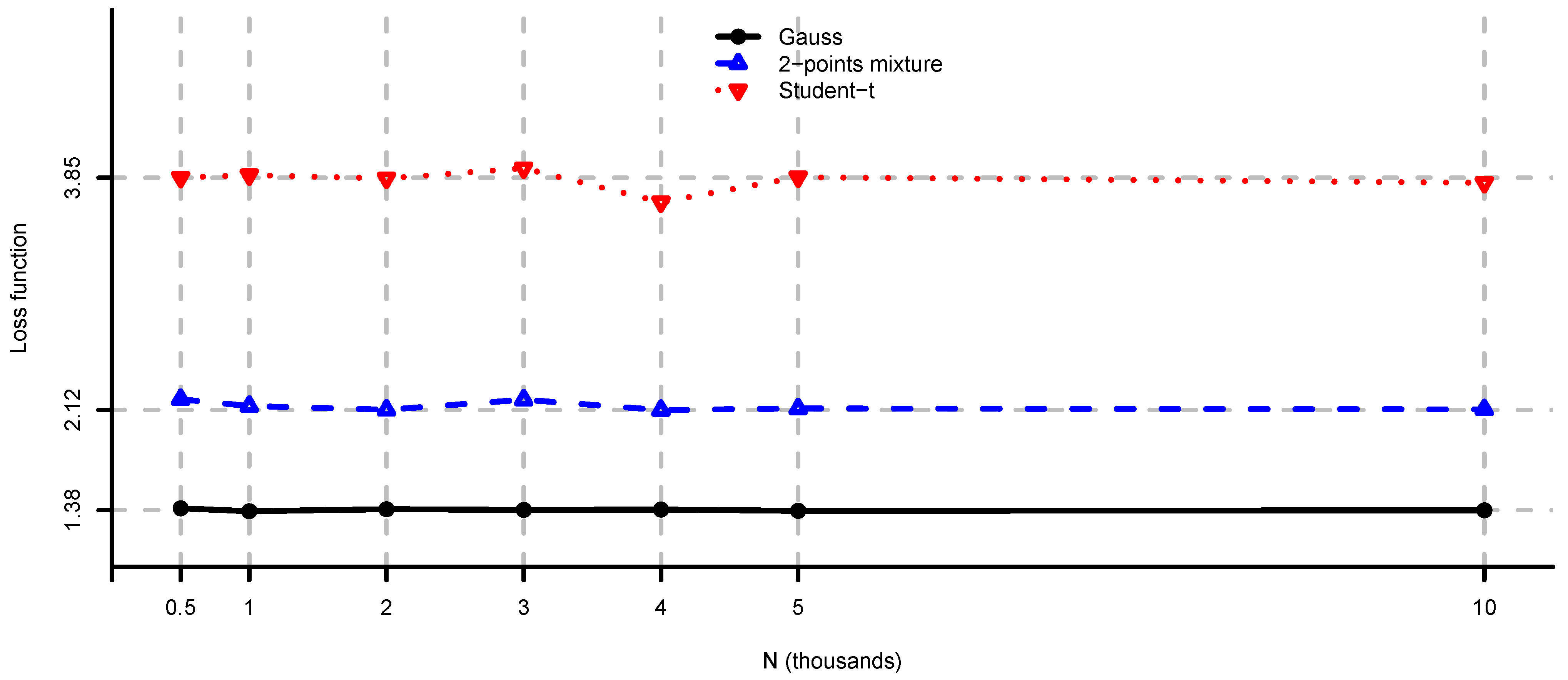
If we fix the number of assets n and let $m\to \infty$ we obtain

$$L(U^{\mathrm{mv}},{\widehat{U}}^{\mathrm{mv}},{\mathbb{R}}^n)⟶\frac{1}{4\kappa }\left(E\left[W^{-2}\right]-E\left[W^{-1}\right]\right){\mathit{\mu }}^{\prime }{\Sigma }^{-1}\mathit{\mu }\ge 0$$

In particular, in the multivariate Gaussian, case we have $L(U^{\mathrm{mv}},{\widehat{U}}^{\mathrm{mv}},{\mathbb{R}}^n)\to 0$ as $m\to \infty$, see Example 2(i).

(iii)

For $n,m\to \infty$ and $n/m\to c\in (0,1)$ we get

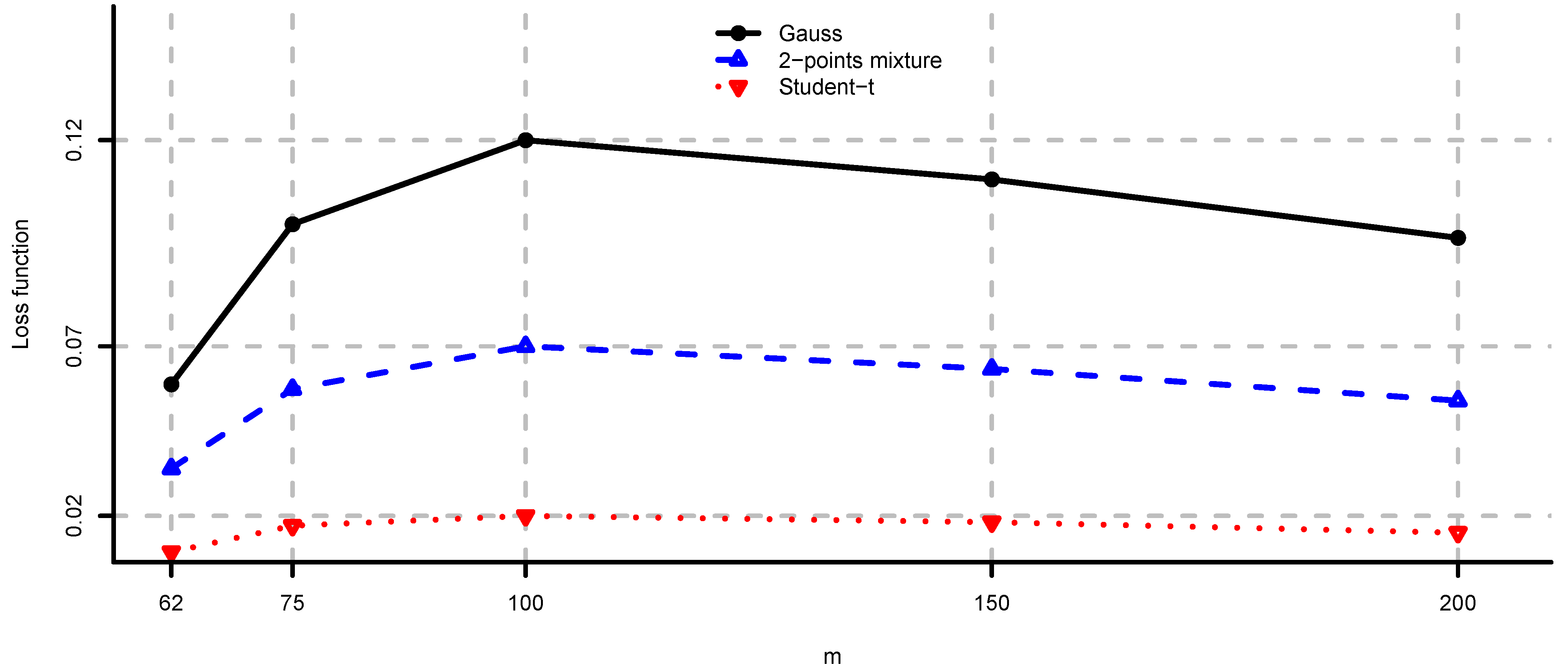
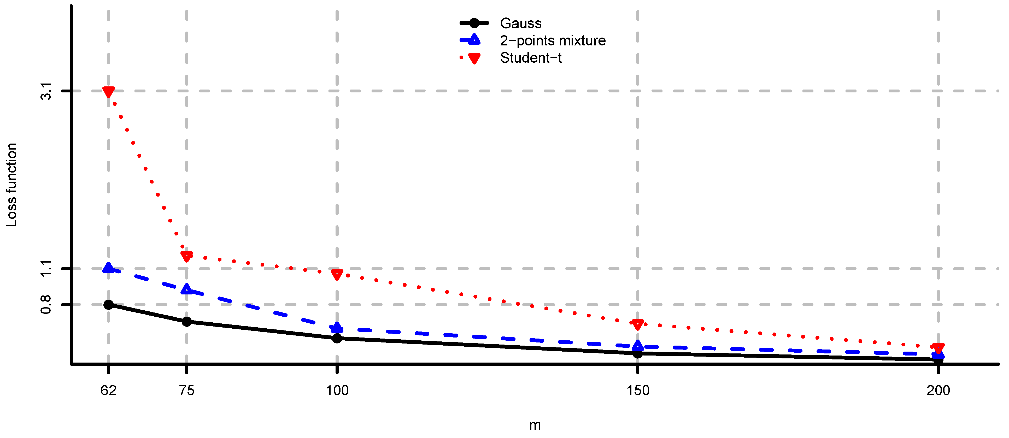
$$\begin{array}{cc}\hfill L(U^{\mathrm{mv}},{\widehat{U}}^{\mathrm{mv}},{\mathbb{R}}^n)& ⟶\frac{1}{4\kappa }\frac{1}{(1-c)}\{c+\frac{c}{{(1-c)}^2}E\left[W^{-1}\right]\hfill \\ & +\left(\frac{1}{{(1-c)}^2}E\left[W^{-2}\right]-E\left[W^{-1}\right]\right){\mathit{\mu }}^{\prime }{\Sigma }^{-1}\mathit{\mu }\}\hfill \end{array}$$

This asymptotic analysis corresponds to large number of risky assets n and comparable sample size m. This limit is considered in El Karoui [29,30] to obtain asymptotic results on model uncertainty in a problem with constraints. The same limit is also considered in Ledoit and Wolf [35] to study asymptotic properties of the spectrum of $\widehat{\Sigma }$. In this paper, we have an explicit characterization of model uncertainty for finite n and m. Note that for $c\to 0^{+}$ we obtain the same limit as in (ii), and for $c\to 1^{-}$ we have $L(U^{\mathrm{mv}},{\widehat{U}}^{\mathrm{mv}},{\mathbb{R}}^n)\to \infty$.

(iv)

Note that the loss function depends on the unobservable distribution of W, true mean vector μ and true covariance matrix Σ.

We consider the special cases for W discussed in Example 2 (see Appendix 1.3).

Corollary 1. 

Let $m>n+4$. In the three special cases given in Example 2 we have for the loss function

(i)

multivariate Gauss:

$$\begin{array}{cc}\hfill L^{\mathrm{Gauss}}(U^{\mathrm{mv}},{\widehat{U}}^{\mathrm{mv}},{\mathbb{R}}^n)& =\frac{1}{4\kappa }\alpha (m-1,n)\{\frac{n}{m}\left(1+\beta (m-1,n)\right)\hfill \\ & +\left(\beta (m-1,n)-1\right){\mathit{\mu }}^{\prime }{\Sigma }^{-1}\mathit{\mu }\}\hfill \end{array}$$

(ii)

2-points mixture:

$$\begin{array}{cc}\hfill L^{2\mathrm{pm}}(U^{\mathrm{mv}},{\widehat{U}}^{\mathrm{mv}},{\mathbb{R}}^n)& =\frac{1}{4\kappa }\alpha (m-1,n)\{\frac{n}{m}-\left(\frac{p}{x_1}+\frac{{(1-p)}^2}{1-p{x}_1}\right){\mathit{\mu }}^{\prime }{\Sigma }^{-1}\mathit{\mu }\hfill \\ & +\frac{n}{m}\beta (m-1,n)\left(\frac{p}{x_1}+\frac{{(1-p)}^2}{1-p{x}_1}\right)\hfill \\ & +\beta (m-1,n)\left(\frac{p}{x_1^2}+\frac{{(1-p)}^3}{{(1-p{x}_1)}^2}\right){\mathit{\mu }}^{\prime }{\Sigma }^{-1}\mathit{\mu }\}\hfill \end{array}$$

where $p\in (0,1)$ and $x_1\in (0,p^{-1})$;

(iii)

multivariate Student-t:

$$\begin{array}{cc}\hfill L^{\mathrm{t}}(U^{\mathrm{mv}},{\widehat{U}}^{\mathrm{mv}},{\mathbb{R}}^n)& =\frac{1}{4\kappa }\alpha (m-1,n)\{\frac{n}{m}\left(1+\beta (m-1,n)\frac{\nu }{\nu -2}\right)\hfill \\ & +\frac{\nu }{\nu -2}\left(\beta (m-1,n)\frac{2+\nu }{\nu -2}-1\right){\mathit{\mu }}^{\prime }{\Sigma }^{-1}\mathit{\mu }\}\hfill \end{array}$$

where $\nu >2$.

Remark 9. 

From the results of Corollary 1 we observe the following facts.

(i)

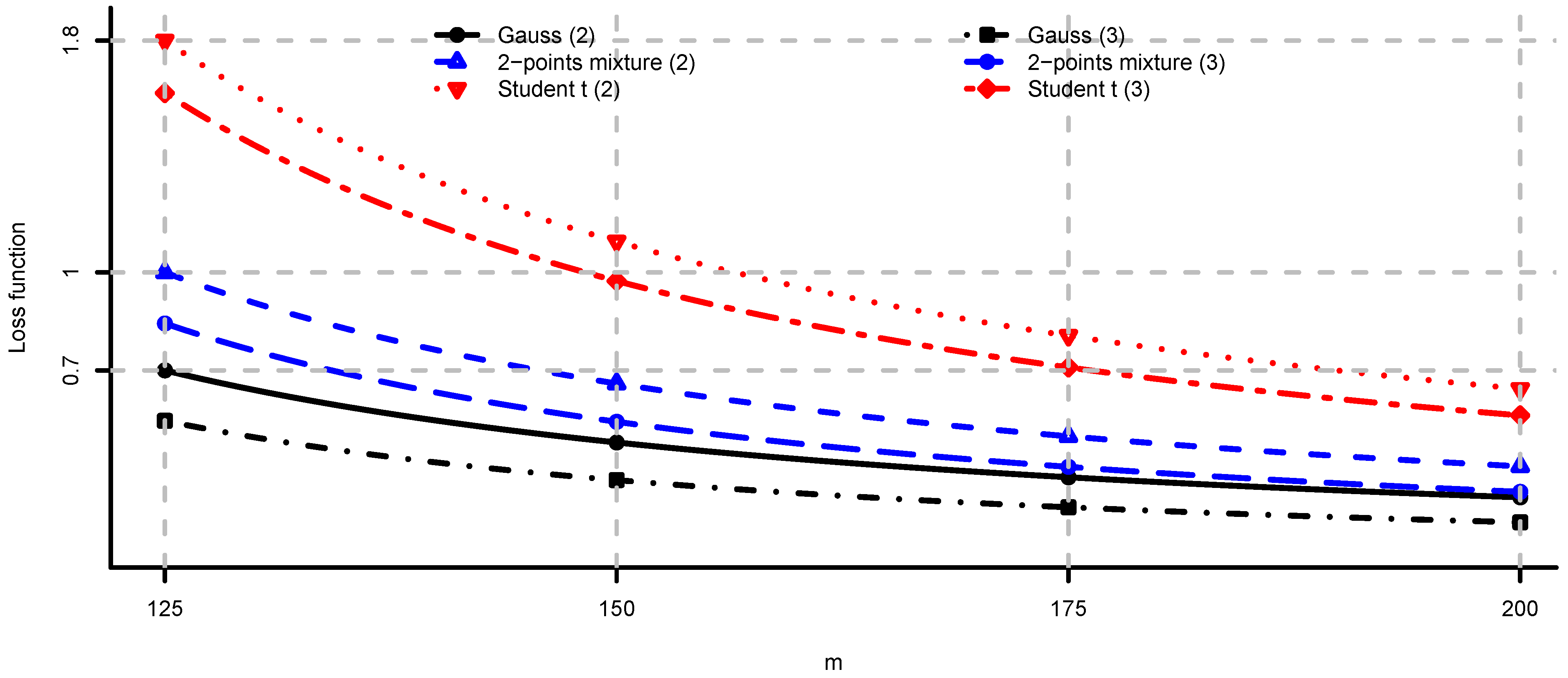
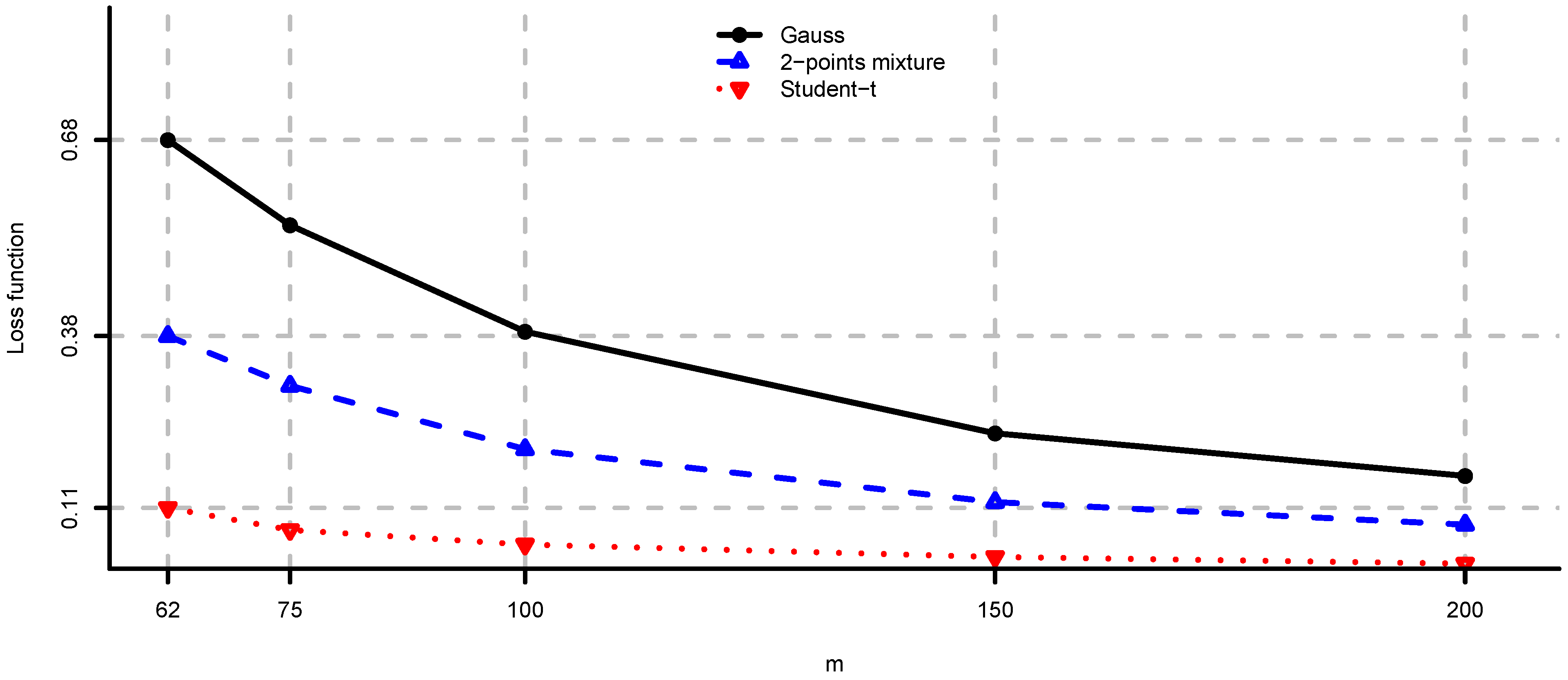
In the 2-points mixture model we have $L^{2\mathrm{pm}}(U^{\mathrm{mv}},{\widehat{U}}^{\mathrm{mv}},{\mathbb{R}}^n)\to \infty$ for $x_1\to p^{-1}$ or $x_1\to 0$, and $L^{2\mathrm{pm}}(U^{\mathrm{mv}},{\widehat{U}}^{\mathrm{mv}},{\mathbb{R}}^n)\to L^{\mathrm{Gauss}}(U^{\mathrm{mv}},{\widehat{U}}^{\mathrm{mv}},{\mathbb{R}}^n)$ for $x_1\to 1$. The more we increase the difference between the two variance regimes (i.e., by considering $x_1\to p^{-1}$ or $x_1\to 0$), the greater the average negative effect of model risk. If we decrease the difference (by considering $x_1\to 1$), then the loss function becomes closer to the Gaussian case.

(ii)

In the multivariate Student-t model we have $L^{\mathrm{t}}(U^{\mathrm{mv}},{\widehat{U}}^{\mathrm{mv}},{\mathbb{R}}^n)\to \infty$ for $\nu \to 2^{+}$, and $L^{\mathrm{t}}(U^{\mathrm{mv}},{\widehat{U}}^{\mathrm{mv}},{\mathbb{R}}^n)\to L^{\mathrm{Gauss}}(U^{\mathrm{mv}},{\widehat{U}}^{\mathrm{mv}},{\mathbb{R}}^n)$ for $\nu \to \infty$. This means, by making the marginals “less normal” (i.e., by considering $\nu \to 2^{+}$), we increase the average negative effect of model risk.

We show that the drawbacks of model uncertainty in the general case are on average bigger than those in the Gaussian case (see Appendix 1.4).

Corollary 2. 

Let $m>n+4$. Then, $L(U^{\mathrm{mv}},{\widehat{U}}^{\mathrm{mv}},{\mathbb{R}}^n)>L^{\mathrm{Gauss}}(U^{\mathrm{mv}},{\widehat{U}}^{\mathrm{mv}},{\mathbb{R}}^n)$, for any $W\ne 1$.

In the financial market asset returns show non-Gaussian behavior, which on average has a negative effect on the optimal portfolio choice. In the next section we consider techniques to reduce the loss function and improve the optimal portfolio.

4. Adjusting for Model Risk

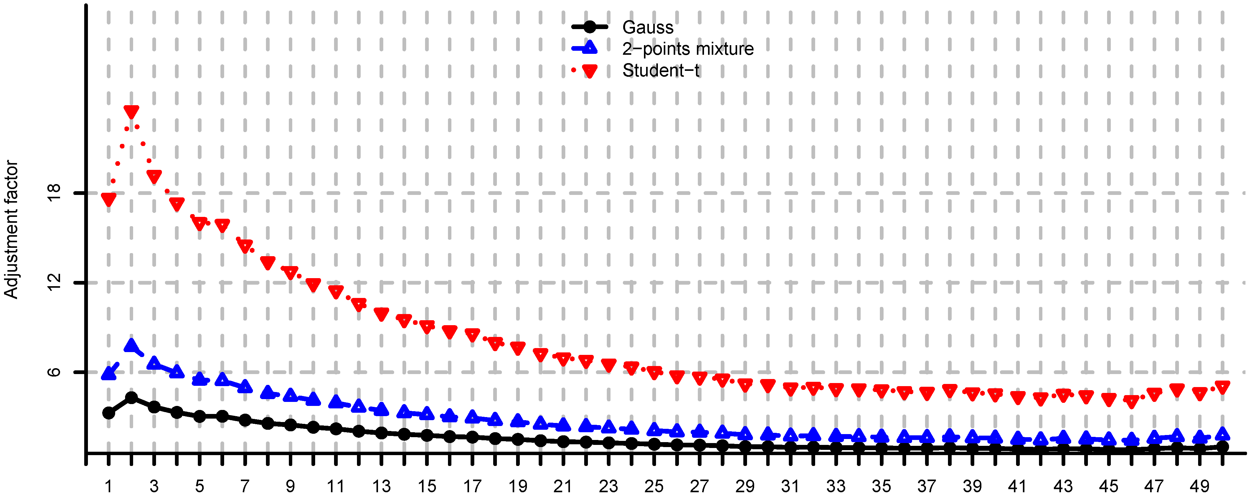
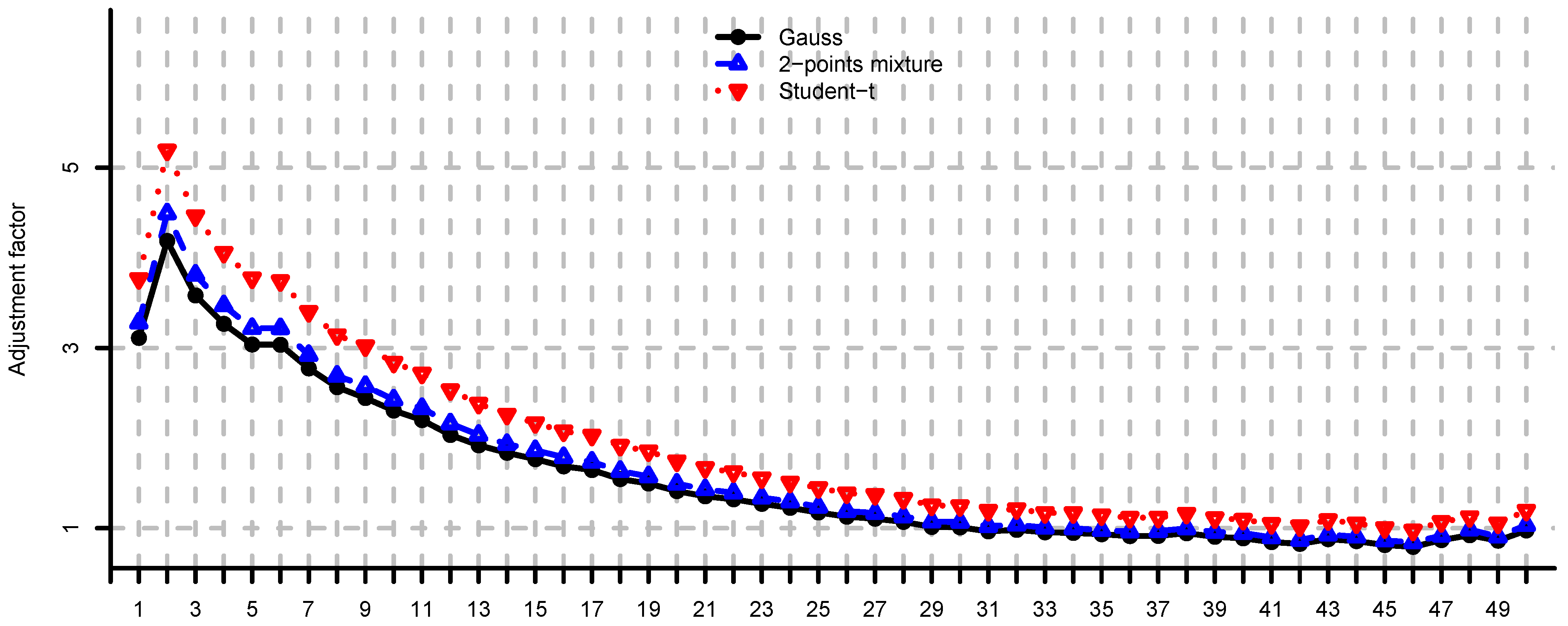
As Proposition 1 and Remark 8(i) pointed out, if we solve the mean-variance problem using the unbiased utility estimator ${\widehat{U}}^{\mathrm{mv}}$, model risk deteriorates the investor’s optimal portfolio choice ${\mathit{w}}^{*}({\widehat{U}}^{\mathrm{mv}},{\mathbb{R}}^n)$. Therefore, we might want to introduce a bias correction in ${\widehat{U}}^{\mathrm{mv}}$ which allows to reduce the loss function (2). In the literature we can find several papers using this idea to improve the optimal portfolio under loss function (3). See for example Jobson et al. [17], Jorion [18], Frost and Savarino [19], Mori [23], and Kan and Zhou [21]. These approaches typically result in rescaled or shrinkage estimators for the mean or covariance matrix so that loss function (3) is improved. In this work, we present an alternative approach based on the classical spectral decomposition of symmetric positive definite matrices.

Remark 10. 

Contrary to Section 3, we do not make specific distributional assumptions on R in the following results, unless explicitly specified.

Let ${\mathit{R}}_1,\dots ,{\mathit{R}}_m\in {\mathcal{L}}^2{(\Omega ,\mathcal{F},P)}^n$, and $\widehat{\mathit{\mu }}$ and $\widehat{\Sigma }$ be unbiased estimators for μ and Σ. We assume that $\widehat{\Sigma }$ is positive definite almost surely. We want to analyze a class of estimators for the covariance matrix Σ obtained by individually rescaling the eigenvalues of $\widehat{\Sigma }$. An asymptotic analysis of this approach is proposed in Ledoit and Wolf [35]. In [35] this is done to improve the covariance matrix estimation without specific considerations on mean-variance optimization. Menchero et al. [38] analyze empirically spectral properties of $\widehat{\Sigma }$ in the context of mean-variance optimization. The spectral decomposition of the symmetric positive definite covariance matrix Σ is given by

$$\Sigma =T\Lambda T^{\prime }$$

where

(i)

$\Lambda =\mathrm{diag}({\lambda }_1,\dots ,{\lambda }_n)$ is the diagonal matrix of eigenvalues (also called eigenvariances in this context) of Σ, which satisfy $0<{\lambda }_1\le \dots \le {\lambda }_n$; and

(ii)

T is an orthogonal matrix with columns $v_1={(T_{11},\dots ,T_{n1})}^{\prime },\dots ,v_n={(T_{n1},\dots ,T_{nn})}^{\prime }$ being the eigenvectors (also called eigenportfolios) of Σ corresponding to ${\lambda }_1,\dots ,{\lambda }_n$, respectively.

In the same way set $\widehat{\Sigma }=\widehat{T}\widehat{\Lambda }{\widehat{T}}^{\prime }$, where $\widehat{T}=({\widehat{v}}_1,\dots ,{\widehat{v}}_n)$ and $\widehat{\Lambda }=\mathrm{diag}({\widehat{\lambda }}_1,\dots ,{\widehat{\lambda }}_n)$ are random matrices with $\widehat{T}{\widehat{T}}^{\prime }=I_n$ and $0<{\widehat{\lambda }}_1\le \dots \le {\widehat{\lambda }}_n$, almost surely. Note that $\widehat{T}$ and $\widehat{\Lambda }$ are in general dependent. In this work we study the following class of covariance matrix estimators

$${\widehat{\Sigma }}_C=\widehat{T}\mathrm{diag}(c_1{\widehat{\lambda }}_1,\dots ,c_n{\widehat{\lambda }}_n){\widehat{T}}^{\prime }$$

where $c_1,\dots ,c_n>0$ are referred to as adjustment factors. For finite n and m, there is only little known about the distribution of $\widehat{\Lambda }$ and $\widehat{T}$. Nevertheless, the decomposition of the sample covariance matrix using eigenportfolios and eigenvariances is a useful tool in mean-variance optimization. It is understood that the eigenvalues of $\widehat{\Sigma }$ behave very differently from those of Σ. Ledoit and Wolf [26] point out that the largest sample eigenvalues are systematically biased upwards and the smallest ones downwards. This fact has also been verified for market return data in different empirical studies, see e.g., Menchero et al. [38]. There is statistical literature studying asymptotic spectral properties of $\widehat{\Sigma }$ when n and m are large, see e.g., Johnstone [33] and El Karoui [29].

Remark 11. 

Note that for any $c_1,\dots ,c_n>0$ the estimator ${\widehat{\Sigma }}_C$ is almost surely positive definite and

$$\begin{array}{cc}\hfill {\widehat{\Sigma }}_C& =\left(\widehat{T}C{\widehat{T}}^{\prime }\right)\widehat{\Sigma }=\widehat{\Sigma }\left(\widehat{T}C{\widehat{T}}^{\prime }\right),\hfill \\ \hfill {\widehat{\Sigma }}_C^{-1}& =\left(\widehat{T}{C}^{-1}{\widehat{T}}^{\prime }\right){\widehat{\Sigma }}^{-1}={\widehat{\Sigma }}^{-1}\left(\widehat{T}{C}^{-1}{\widehat{T}}^{\prime }\right)\hfill \end{array}$$

where $C=\mathrm{diag}(c_1,\dots ,c_n)$. If $C=I_n$ then ${\widehat{\Sigma }}_C$ is unbiased for Σ.

Using ${\widehat{\Sigma }}_C$ we define the following utility estimator for $\mathit{w}\in {\mathbb{R}}^n$

$${\widehat{U}}_C^{\mathrm{mv}}\left(\mathit{w}\right)={\widehat{\mathit{\mu }}}^{\prime }\mathit{w}-\kappa \mathit{w}{\widehat{\Sigma }}_C\mathit{w}={\widehat{\mathit{\mu }}}^{\prime }\mathit{w}-\kappa \mathit{w}\left(\widehat{T}C{\widehat{T}}^{\prime }\right)\widehat{\Sigma }\mathit{w}$$

Our aim is to determine adjustment factors $c_1,\dots ,c_n$ so that

$$L(U^{\mathrm{mv}},{\widehat{U}}_C^{\mathrm{mv}},\widehat{\mathcal{A}})\le L(U^{\mathrm{mv}},{\widehat{U}}^{\mathrm{mv}},\widehat{\mathcal{A}})$$

(6)

see also Proposition 1. In this way we obtain an optimal portfolio ${\mathit{w}}^{*}({\widehat{U}}_C^{\mathrm{mv}},\widehat{\mathcal{A}})$ which is more robust to model uncertainty as measured by Equation (2). We can accomplish this in a straightforward way considering the special case of equal adjustment factors (see Appendix 1.5).

Proposition 3. 

Choose $c_1=\dots =c_n=\overline{c}>0$. Let ${\Sigma }_{\overline{c}}={\widehat{\Sigma }}_C=\overline{c}\widehat{\Sigma }$ and ${\widehat{U}}_{\overline{c}}^{\mathrm{mv}}$ be the corresponding utility estimator. Then,

$$L(U^{\mathrm{mv}},{\widehat{U}}_{\overline{c}}^{\mathrm{mv}},{\mathbb{R}}^n)=\frac{1}{4\overline{c}\kappa }E\left[{\widehat{\mathit{\mu }}}^{\prime }{\widehat{\Sigma }}^{-1}\widehat{\mathit{\mu }}\right]-\frac{1}{2\overline{c}\kappa }{\mathit{\mu }}^{\prime }E\left[{\widehat{\Sigma }}^{-1}\widehat{\mathit{\mu }}\right]+\frac{1}{4{\overline{c}}^2\kappa }E\left[{\widehat{\mathit{\mu }}}^{\prime }{\widehat{\Sigma }}^{-1}\Sigma {\widehat{\Sigma }}^{-1}\widehat{\mathit{\mu }}\right]$$

In particular, under assumption Equation (4) on the observations, and setting

$$\overline{c}=\beta (m-1,n)\frac{E\left[W^{-2}\right]}{E\left[W^{-1}\right]}$$

(7)

we have $L(U^{\mathrm{mv}},{\widehat{U}}_{\overline{c}}^{\mathrm{mv}},{\mathbb{R}}^n)\le L(U^{\mathrm{mv}},{\widehat{U}}^{\mathrm{mv}},{\mathbb{R}}^n)$.

Remark 12. 

Observe the following about the approach of Proposition 3.

(i)

${\widehat{\Sigma }}_{\overline{c}}=\overline{c}\widehat{\Sigma }$ is a simple proportional scaling type estimator. The unconstrained mean-variance portfolio constructed using ${\widehat{\Sigma }}_{\overline{c}}$ is given by

$${\mathit{w}}^{*}({\widehat{U}}_{\overline{c}}^{\mathrm{mv}},{\mathbb{R}}^n)=\frac{1}{2\overline{c}\kappa }{\widehat{\Sigma }}^{-1}\widehat{\mathit{\mu }}$$

(8)

(ii)

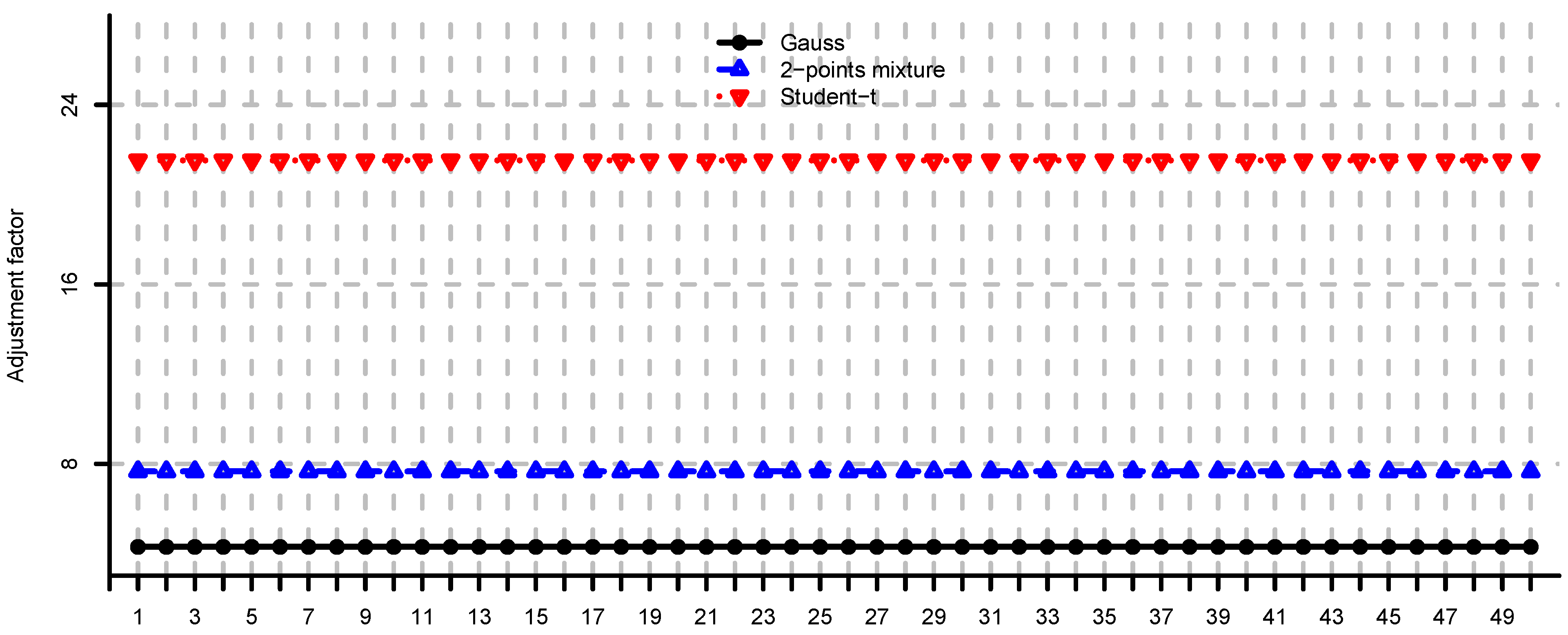
In general, adjustment factors (7) are unobservable since they depend on the unknown distribution of W. Note that, by Remark 8(i) we have

$$\overline{c}\ge \beta (m-1,n)$$

with equality in the multivariate Gaussian case.

Scaling $\widehat{\Sigma }$ by $\overline{c}$ is useful since it reduces the impact of model risk. However, this proportional scaling is not helpful to improve the relative asset allocation because it does not adjust the correlation structure of $\widehat{\Sigma }$. For example, in the unconstrained mean-variance case, all portfolio weights are uniformly reduced by a constant factor $1/\overline{c}$, i.e., the risk aversion is increased by factor $\overline{c}$, see Equation (7). Since the relative asset allocation remains the same, this cannot be considered as a substantial improvement in the optimal portfolio allocation. Therefore, we consider individual adjustment factors $c_1,\dots ,c_n$ for the eigenvariances ${\widehat{\lambda }}_1,\dots ,{\widehat{\lambda }}_n$.

A heuristic approach to select the adjustment factors is to set for $k=1,\dots ,n$

$$c_k=\frac{{\lambda }_k}{E\left[{\widehat{\lambda }}_k\right]}$$

(9)

This rule ensures that the eigenvariances of ${\widehat{\Sigma }}_C$ are unbiased estimators for the ones of Σ.

In the next result we calculate $L(U^{\mathrm{mv}},{\widehat{U}}_C^{\mathrm{mv}},{\mathbb{R}}^n)$ for general $c_1,\dots ,c_n$ in the unconstrained mean-variance case (see Appendix 1.6). We first introduce some additional notation to simplify the representation. Since the family $\{v_1,\dots ,v_n\}$ of eigenportfolios builds an orthonormal basis for ${\mathbb{R}}^n$ we can write the optimal portfolio as

$${\mathit{w}}^{*}({\widehat{U}}^{\mathrm{mv}},\widehat{\mathcal{A}})=\sum _{k=1}^n{\pi }_k\left({\mathit{w}}^{*}({\widehat{U}}^{\mathrm{mv}},\widehat{\mathcal{A}}),\Sigma \right)v_k$$

where ${\pi }_k(\mathit{w},\Sigma )={\left(T^{\prime }\mathit{w}\right)}_k$ denotes the projection of $\mathit{w}\in {\mathbb{R}}^n$ on the eigenportfolio $v_k$. In the same way we define ${\pi }_k(\mathit{w},\widehat{\Sigma })$ and ${\pi }_k(\mathit{w},{\widehat{\Sigma }}_C)$. Note that, in general, these two random variables depend on both $\widehat{T}$ and $\widehat{\Lambda }$.

Theorem 4. 

The loss function for the unconstrained mean-variance problem and the estimator ${\widehat{\Sigma }}_C$ is given by

$$\begin{array}{cc}\hfill L(U^{\mathrm{mv}},{\widehat{U}}_C^{\mathrm{mv}},{\mathbb{R}}^n)& =\frac{1}{2\kappa }\sum _{k=1}^{n}E\left[\left({\pi }_k{(\widehat{\mathit{\mu }},\widehat{\Sigma })}^2-{\pi }_k(\widehat{\mathit{\mu }},\widehat{\Sigma }){\pi }_k(\mathit{\mu },\widehat{\Sigma })\right)c_k^{-1}{\widehat{\lambda }}_k^{-1}\right]\hfill \\ & +\frac{1}{4\kappa }\sum _{k=1}^{n}E\left[{\pi }_k{({\widehat{\Sigma }}_C^{-1}\widehat{\mathit{\mu }},\Sigma )}^2{\lambda }_k-{\pi }_k{(\widehat{\mathit{\mu }},\widehat{\Sigma })}^2{c}_k^{-1}{\widehat{\lambda }}_k^{-1}\right]\hfill \end{array}$$

From the general formula of Theorem 4 it is difficult to derive a simple rule to select the adjustment factors $c_1,\dots ,c_n$. However, this can be done under the following simplifying assumptions. For the estimators $\widehat{\mathit{\mu }}$ and $\widehat{\Sigma }$ we consider the following assumption

$$\widehat{\Sigma }=T\widehat{\Lambda }{T}^{\prime }$$

(10)

where

(i)

$\widehat{\Lambda }=\mathrm{diag}({\widehat{\lambda }}_1,\dots ,{\widehat{\lambda }}_n)$ independent of $\widehat{\mathit{\mu }}$,

(ii)

$0<{\widehat{\lambda }}_1\le \dots \le {\widehat{\lambda }}_n$ almost surely and integrable, and

(iii)

$E\left[\widehat{\mathit{\mu }}\right]=\mathit{\mu }$.

This means that we consider only estimation uncertainty in the means and eigenvariances, and assume independence between eigenvariances and means.

Remark 13. 

The estimator $\widehat{\Sigma }$ is almost surely positive definite by assumption. The estimator $\widehat{\Sigma }$ is unbiased for Σ if and only if $\widehat{\Lambda }$ is unbiased for Λ.

We derive the following result for the loss function (see Appendix 1.7).

Theorem 5. 

Under Equation (10) we have

$$\begin{array}{cc}\hfill L(U^{\mathrm{mv}},{\widehat{U}}_C^{\mathrm{mv}},{\mathbb{R}}^n)& =\frac{1}{2\kappa }\sum _{k=1}^n{c}_k^{-1}\mathrm{Var}\left[{\pi }_k(\widehat{\mathit{\mu }},\Sigma )\right]E\left[{\widehat{\lambda }}_k^{-1}\right]\hfill \\ & +\frac{1}{4\kappa }\sum _{k=1}^{n}E\left[{\pi }_k{(\widehat{\mathit{\mu }},\Sigma )}^2\right]\left(c_k^{-2}E\left[{\widehat{\lambda }}_k^{-2}\right]{\lambda }_k-c_k^{-1}E\left[{\widehat{\lambda }}_k^{-1}\right]\right)\hfill \end{array}$$

Assume $\widehat{\Sigma }$ is unbiased for Σ and set

$$c_k=\frac{{\lambda }_{k}E\left[{\widehat{\lambda }}_k^{-2}\right]}{E\left[{\widehat{\lambda }}_k^{-1}\right]}$$

(11)

Then, $c_k\ge 1$ for all $k=1,\dots ,n$ and $L(U^{\mathrm{mv}},{\widehat{U}}_C^{\mathrm{mv}},{\mathbb{R}}^n)\le L(U^{\mathrm{mv}},{\widehat{U}}^{\mathrm{mv}},{\mathbb{R}}^n)$.

In the simplified situation (10) we obtain a rule for selecting the adjustment factors $c_1,\dots ,c_n$ which reduces the effects of model risk.

In Section 5 we show that adjustment factors (7), (9) and (11) considerably reduce the loss function (2) in the mean-variance problem. This reduction is particularly large in the multivariate Student-t case with small values of ν, or in the case when n is close to m. The numerical results show that the adjustment factors (11) reduce the drawbacks of model uncertainty also when we use the sample estimator for the covariance matrix. We interpret this fact as the property that estimation errors in the eigenportfolios and eigenvariances of the sample covariance matrix may have low correlation with each other. Therefore, selecting the adjustment factors based on the stand-alone effect of estimation uncertainty in the eigenvariances is helpful. Note that the adjustment factors (7), (9) and (11) are, in general, not observable and need to be estimated. This issue is also addressed in Section 5.

5. Case Studies

5.1. Simulated Observations

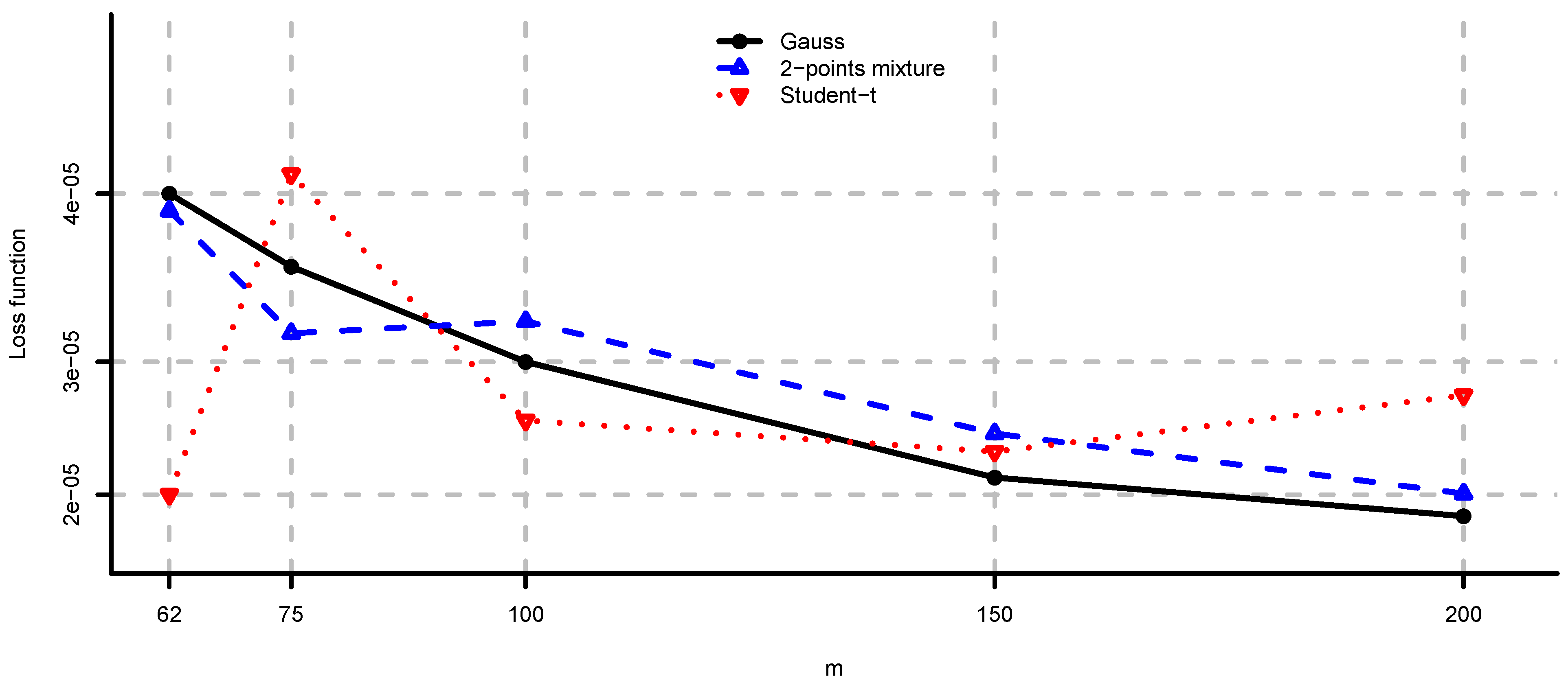
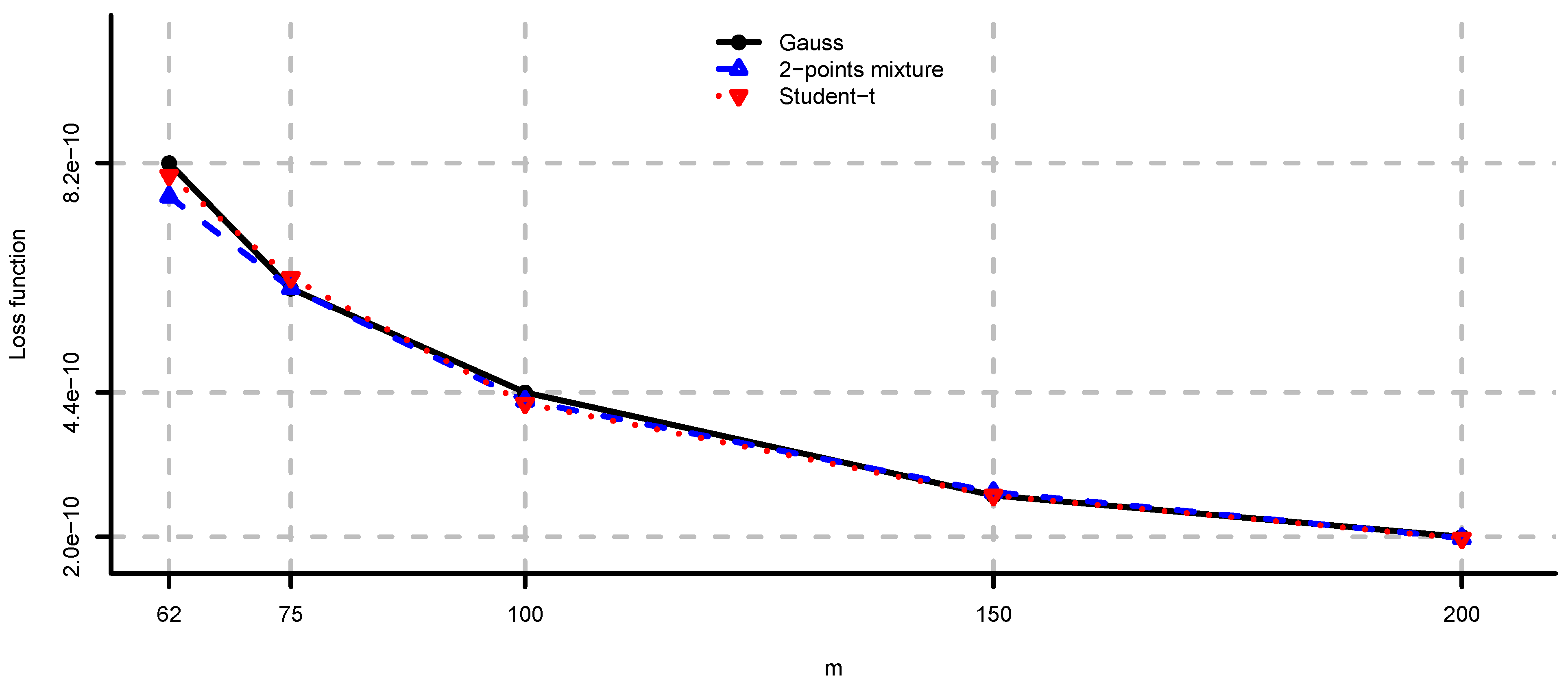
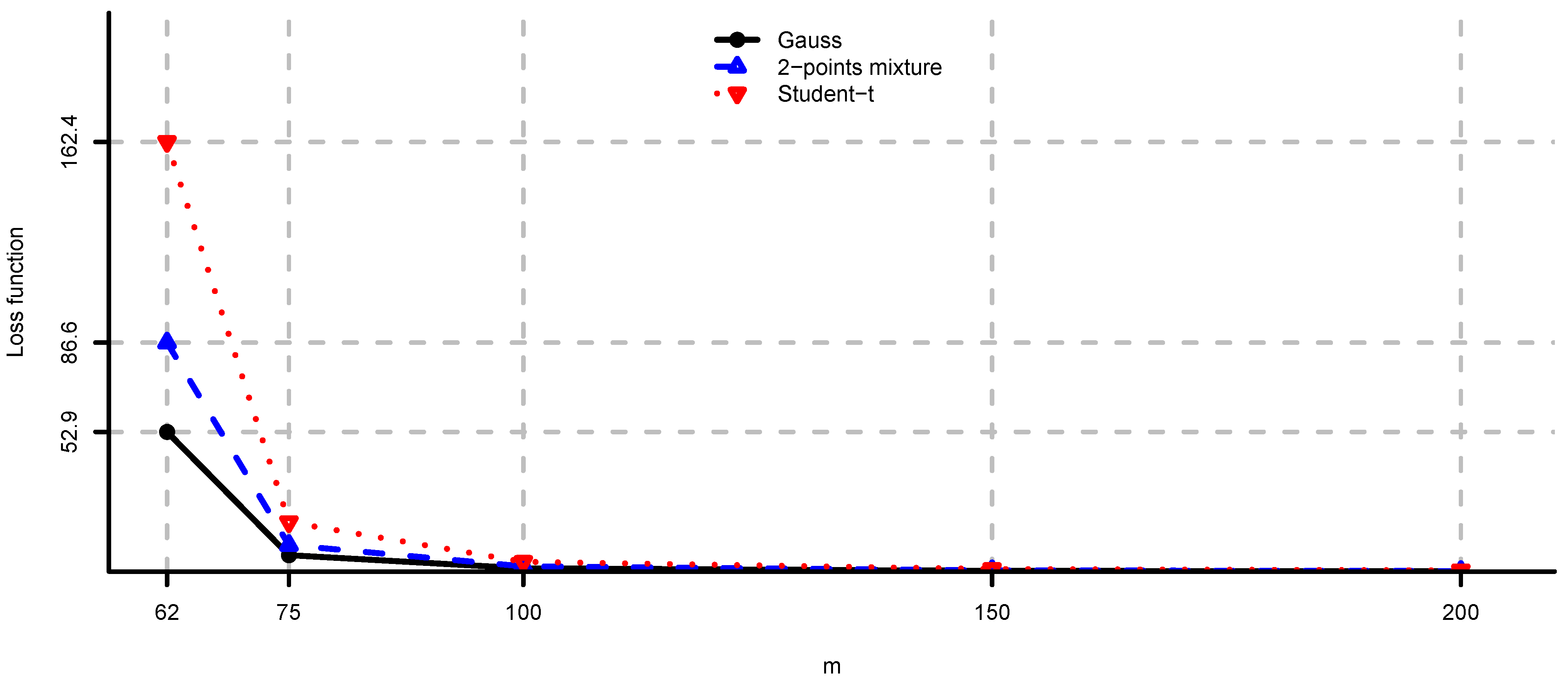
In the first place we compute loss function (2) using return observations simulated from known μ and Σ. We consider the following four problems, see Example 1.

(i)

Unconstrained mean-variance: $U=U^{\mathrm{mv}}$ and $\mathcal{A}={\mathbb{R}}^n$. We set $\kappa =1$ for the risk aversion parameter.

(ii)

Long only fully invested minimum variance: $U=U^{\mathrm{v}}$ and $\mathcal{A}=\{\mathit{w}\in {\mathbb{R}}^n|{\mathbf{1}}^{\prime }\mathit{w}=1\text{and}{w}_i\ge 0\text{for}\text{all}i=1,\dots ,n\}$.

(iii)

Long only fully invested equal contributions to risk: $U=U^{\mathrm{ecr}}$ and $\mathcal{A}$ as in (ii).

(iv)

Long only fully invested maximum diversification: $U=U^{\mathrm{md}}$ and $\mathcal{A}$ as in (ii).

We set $n=50$ assets and consider different values for the number of observations m. We set μ and Σ equal to the sample estimates computed from the dataset of Section 5.2. We simulate independently N samples of m return observations from the three distributional models of Example 2. In the 2-points mixture case we set $x_1=5$ and $p=0.1$; in the multivariate Student-t case we set $\nu =3$.

In Figure 1 and Figure 2 we see the values of loss function (2) in the unconstrained mean-variance problem (i). As N becomes larger we have convergence to the values given by Theorem 2. Note also that, as expected by Corollary 2, the drawbacks of model risk are considerably more severe in the 2-points mixture and the multivariate Student-t models compared to the multivariate Gaussian case. We observe that the loss function is decreasing in the sample size m, steep for m close to n and flat for $m\gg n$. From this analysis we conclude that the unconstrained mean-variance portfolio is severely compromised by model risk and particularly so in the case of non-Gaussian returns and m close to n. An adjustment in the sense of Section 4 is therefore necessary in this problem.

Figure 1. $L^{\mathrm{Gauss}}(U^{\mathrm{mv}},{\widehat{U}}^{\mathrm{mv}},{\mathbb{R}}^n)$, $L^{2\mathrm{pm}}(U^{\mathrm{mv}},{\widehat{U}}^{\mathrm{mv}},{\mathbb{R}}^n)$ and $L^{\mathrm{t}}(U^{\mathrm{mv}},{\widehat{U}}^{\mathrm{mv}},{\mathbb{R}}^n)$ computed by simulation for $n=50$, $m=100$ and different values of N. The values given by Theorem 2 are approximately $1.3814$, $2.1236$ and $3.8453$, respectively.

Figure 2. $L(U^{\mathrm{mv}},{\widehat{U}}^{\mathrm{mv}},{\mathbb{R}}^n)$ computed using Theorem 2 for $n=50$ and different values of m.

In Figure 3 we compare the loss functions (2) and (3). Using similar arguments as in Appendix 1.2 we also have a closed-form expression for Equation (3). As expected from Remark 4 we see that (2) is larger than (3) for each model. We observe that the additional positive component in Equation (2) is not negligible.

In Figure 4, Figure 5 and Figure 6 we provide loss function (2) in problem (i) using the covariance matrix estimator ${\widehat{\Sigma }}_C$, where $c_1,\dots ,c_n$ are chosen according to Equations (7), (9) and (11). Note that rule (7) simply increases the risk aversion, rule (9) is a heuristic approach and rule (11) is derived under simplifying assumptions. These estimators provide a significant reduction in the loss function, in particular for small m, compare Figure 4, Figure 5 and Figure 6 to Figure 2. We conclude that using the adjustment factors of Section 4 we obtain optimal portfolios which are more robust to model risk. In practice, the adjustment factors (7), (9) and (11) need to be estimated, and therefore the loss function improvement is less pronounced. Observe that the loss function curves in Figure 4, Figure 5 and Figure 6 are less steep for m close to n compared to Figure 2. In Figure 7, Figure 8 and Figure 9 we show the adjustment factors computed for each eigenvariance. For adjustment factors Equation (7) we have constant scaling (see Figure 7), and for adjustment factors (9) and (11) each eigenvariance is scaled individually (see Figure 8 and Figure 9). In Figure 8 we also observe the stylized facts of Ledoit and Wolf [26], and Menchero et al. [38], i.e., small eigenvariances are substantially biased downwards and large eigenvariances are slightly biased.

Figure 3. Loss functions (2) and (3) for $n=50$ and different values of m.

Figure 4. $L(U^{\mathrm{mv}},{\widehat{U}}_C^{\mathrm{mv}},{\mathbb{R}}^n)$ computed by simulation ($N=1000$) for $n=50$ and different values of m. The adjustment factors $c_1,\dots ,c_n$ are selected according to Equation (7).

Figure 5. As in Figure 4 where $c_1,\dots ,c_n$ are selected according to Equation (9).

Figure 6. As in Figure 4 where $c_1,\dots ,c_n$ are selected according to Equation (11).

Figure 7. Adjustment factors Equation (7) computed by simulation for $N=1000$ and $m=100$, for each eigenvariance.

Figure 8. Adjustment factors (9) computed by simulation for $N=1000$ and $m=100$, for each eigenvariance.

Figure 9. Adjustment factors (11) computed by simulation for $N=1000$ and $m=100$, for each eigenvariance.

Note that problem (i) requires estimation of μ and Σ, whereas problems (ii)–(iv) require only estimation of Σ. We compare the behavior of the loss functions in (ii)–(iv) for different values of m, since they are based on estimation of the same parameters. In Figure 10, Figure 11 and Figure 12 we present these loss functions. We observe that these problems are not severely deteriorated by model risk even in the case of n close to m or non-Gaussian observations because they only require estimation of Σ. The equal contributions to risk and maximum diversification portfolios are less affected by the distribution of the observations compared to the minimum variance portfolio.

Figure 10. $L(U^{\mathrm{v}},U^{\mathrm{v}},\mathcal{A})$ for $N=1000$ and different values of m.

Figure 11. $L(U^{\mathrm{ecr}},U^{\mathrm{ecr}},\mathcal{A})$ for $N=1000$ and different values of m.

Figure 12. $L(U^{\mathrm{md}},U^{\mathrm{md}},\mathcal{A})$ for $N=1000$ and different values of m.

5.2. Large-Cap U.S. Equity Portfolios

We consider an investment universe of 50 large-cap U.S. stocks from different industry sectors. The list of companies is given in Appendix 3. We set $n=50$ and enumerate the companies according to the list. For these stocks we consider daily total returns (i.e., dividends are included) for the period from 2 January 1995 to 14 October 2011 (4380 daily observations). We study the mean-variance optimization problem under long only fully invested constraints, i.e., $\mathcal{A}=\{\mathit{w}\in {\mathbb{R}}^n|{\mathbf{1}}^{\prime }\mathit{w}=1\text{and}{w}_i\ge 0\text{for}\text{all}i=1,\dots ,n\}$, see Example 1(i). In this numerical example we set $\kappa =100$ for the risk aversion parameter. In this way the utility function is mainly determined by the portfolio variance and the problem is comparable to a constrained minimum variance problem, see Example 1(ii). For parameter estimation we use $m=100$, i.e., for each trading day we consider the previous 100 daily observations to estimate μ and Σ. Note that the estimation of μ is required in this problem, unlike in problems (ii)–(iv) of Section 5.1. As shown in Section 5.1, the estimator ${\widehat{\Sigma }}_C$, where $c_1,\dots ,c_n$ are selected according to Equations (7) and (11), considerably reduces the negative effects of model risk in the unconstrained mean-variance problem. In this section we apply Equations (7) and (11) to the problem of long only fully invested constraints. Observe that for non-Gaussian observations the adjustment factors (7) depend on the unobservable distribution of W. To estimate these values we calibrate a specific normal variance mixture model to the data. The adjustment factors (11) are also unobservable since they depend on the true covariance matrix. In order to estimate them we rely on the following simulation procedure. For each trading day, we estimate $\widehat{\Sigma }$ and consider it as the true covariance matrix. We then simulate $N=1000$ samples of 100 observations using a specific normal variance mixture model calibrated to the data. These samples are used, on the other hand, to estimate sample covariance matrices ${\Sigma }^{\left(1\right)},\dots ,{\Sigma }^{\left(N\right)}$. Diagonalization of these matrices provide the eigenvariances

$${\left({\widehat{\lambda }}_i^{\left(j\right)}\right)}_{i=1,\dots ,n,j=1,\dots ,N}$$

which are ordered such that ${\widehat{\lambda }}_1^{\left(j\right)}\le \dots \le {\widehat{\lambda }}_n^{\left(j\right)}$ for all $j=1,\dots ,N$. Then, we set for $i=1,\dots ,n$

$$c_i={\widehat{\lambda }}_i\frac{{\sum }_{k=1}^N{\left({\widehat{\lambda }}_i^{\left(k\right)}\right)}^{-2}}{{\sum }_{k=1}^N{\left({\widehat{\lambda }}_i^{\left(k\right)}\right)}^{-1}}$$

(12)

We perform out-of-sample backtesting of the following five investment strategies, where we set $\kappa =100$ and $\mathcal{A}=\{\mathit{w}\in {\mathbb{R}}^n|{\mathbf{1}}^{\prime }\mathit{w}=1\text{and}{w}_i\ge 0\text{for}\text{all}i=1,\dots ,n\}$.

(i)

The classical mean-variance portfolio ${\mathit{w}}^{*}({\widehat{U}}^{\mathrm{mv}},\mathcal{A})$ based on the sample estimators $\widehat{\mathit{\mu }}$ and $\widehat{\Sigma }$.

(ii)

Portfolio ${\mathit{w}}^{*}({\widehat{U}}_{\overline{c}}^{\mathrm{mv}},\mathcal{A})$ based on the estimators $\widehat{\mathit{\mu }}$ and ${\widehat{\Sigma }}_{\overline{c}}$, where $\overline{c}$ is determined by Equation (7) under a multivariate Gaussian model.

(iii)

As in (ii), where $\overline{c}$ is determined by Equation (7) under a multivariate Student-t model.

(iv)

Portfolio ${\mathit{w}}^{*}({\widehat{U}}_C^{\mathrm{mv}},\mathcal{A})$ based on the estimators $\widehat{\mathit{\mu }}$ and ${\widehat{\Sigma }}_C$, where $c_1,\dots ,c_n$ are determined numerically by Equation (12) under a multivariate Gaussian model.

(v)

As in (iv), where $c_1,\dots ,c_n$ are determined numerically by Equation (12) under a multivariate Student-t model.

In Table 1 and Table 2 we present the out-of-sample backtesting results of investment strategies (i)–(v).

Table 1. Out-of-sample backtesting results of the strategies (i)–(iii). All numbers are expressed in percent except for Sharpe ratios and average degrees of diversification. The return and volatility values are annualized assuming 250 trading days per year.

	Return Annualized			Volatility Annualized			Sharpe Ratio			Maximum Drawdown			Average Turnover			Average Diversification
	(i)	(ii)	(iii)	(i)	(ii)	(iii)	(i)	(ii)	(iii)	(i)	(ii)	(iii)	(i)	(ii)	(iii)	(i)	(ii)	(iii)
All	7.63	8.03	8.66	15.06	15.01	15.00	0.51	0.53	0.58	47.80	47.16	45.31	13.38	12.78	12.25	10.05	10.10	10.15
2011	10.85	11.85	12.01	14.09	13.97	13.88	0.77	0.85	0.87	10.04	9.58	9.75	13.75	12.95	12.31	8.87	8.98	9.05
2010	9.13	9.26	8.90	11.12	10.97	10.86	0.82	0.84	0.82	7.63	7.35	7.33	10.39	9.94	9.80	7.74	7.88	8.05
2009	22.10	21.35	24.27	17.94	18.05	18.19	1.23	1.18	1.33	19.56	20.06	18.83	10.84	10.69	10.28	9.66	9.57	9.54
2008	−27.67	−26.57	−25.93	28.82	28.74	28.91	neg	neg	neg	39.68	38.59	38.05	12.95	12.31	11.60	8.03	7.97	7.94
2007	10.29	10.06	10.72	11.33	11.23	11.09	0.91	0.90	0.97	7.05	6.87	6.70	14.27	13.27	12.80	8.39	8.34	8.38
2006	9.30	10.04	10.91	8.05	7.96	7.89	1.16	1.26	1.38	5.93	5.37	4.78	15.06	13.62	12.40	8.43	8.23	8.03
2005	1.66	2.02	1.94	9.59	9.51	9.41	0.17	0.21	0.21	7.29	6.79	6.62	15.75	15.16	14.48	9.38	9.47	9.53
2004	9.17	9.76	10.38	9.45	9.35	9.26	0.97	1.04	1.12	7.68	7.18	6.79	14.28	13.50	12.59	8.52	8.68	8.86
2003	20.49	21.05	21.44	12.16	12.10	12.07	1.69	1.74	1.78	8.57	8.59	8.80	13.03	12.64	12.05	9.24	9.20	9.15
2002	−13.33	−13.29	−12.20	18.12	18.25	18.26	neg	neg	neg	27.35	27.56	27.19	12.33	12.05	11.74	9.39	9.52	9.56
2001	−7.23	−6.52	−5.41	13.97	13.89	13.94	neg	neg	neg	16.49	16.20	16.00	13.93	13.45	13.14	11.85	11.93	12.02
2000	6.64	6.29	6.83	17.99	17.99	18.01	0.37	0.35	0.38	22.37	22.42	22.34	14.70	14.49	13.95	12.80	12.94	13.00
1999	−2.76	−1.62	−0.41	15.32	15.30	15.25	neg	neg	neg	15.12	14.52	14.01	14.45	13.77	13.47	12.00	12.16	12.35
1998	18.57	19.22	19.09	17.63	17.57	17.61	1.05	1.09	1.08	17.41	17.57	17.88	13.82	13.53	13.35	11.09	10.99	10.92
1997	26.78	26.58	26.09	15.91	15.76	15.59	1.68	1.69	1.67	8.05	8.07	8.13	12.54	11.82	11.12	11.32	11.31	11.25
1996	18.62	19.32	20.01	12.01	11.94	11.88	1.55	1.62	1.68	7.33	7.13	7.17	14.93	14.22	13.70	12.03	12.33	12.61
1995	17.80	18.60	19.35	7.76	7.60	7.47	2.29	2.45	2.59	3.77	3.72	3.78	9.72	9.26	8.83	12.92	13.15	13.40

Table 1. Out-of-sample backtesting results of the strategies (i)–(iii). All numbers are expressed in percent except for Sharpe ratios and average degrees of diversification. The return and volatility values are annualized assuming 250 trading days per year.

	Return Annualized			Volatility Annualized			Sharpe Ratio			Maximum Drawdown			Average Turnover			Average Diversification
	(i)	(ii)	(iii)	(i)	(ii)	(iii)	(i)	(ii)	(iii)	(i)	(ii)	(iii)	(i)	(ii)	(iii)	(i)	(ii)	(iii)
All	7.63	8.03	8.66	15.06	15.01	15.00	0.51	0.53	0.58	47.80	47.16	45.31	13.38	12.78	12.25	10.05	10.10	10.15
2011	10.85	11.85	12.01	14.09	13.97	13.88	0.77	0.85	0.87	10.04	9.58	9.75	13.75	12.95	12.31	8.87	8.98	9.05
2010	9.13	9.26	8.90	11.12	10.97	10.86	0.82	0.84	0.82	7.63	7.35	7.33	10.39	9.94	9.80	7.74	7.88	8.05
2009	22.10	21.35	24.27	17.94	18.05	18.19	1.23	1.18	1.33	19.56	20.06	18.83	10.84	10.69	10.28	9.66	9.57	9.54
2008	−27.67	−26.57	−25.93	28.82	28.74	28.91	neg	neg	neg	39.68	38.59	38.05	12.95	12.31	11.60	8.03	7.97	7.94
2007	10.29	10.06	10.72	11.33	11.23	11.09	0.91	0.90	0.97	7.05	6.87	6.70	14.27	13.27	12.80	8.39	8.34	8.38
2006	9.30	10.04	10.91	8.05	7.96	7.89	1.16	1.26	1.38	5.93	5.37	4.78	15.06	13.62	12.40	8.43	8.23	8.03
2005	1.66	2.02	1.94	9.59	9.51	9.41	0.17	0.21	0.21	7.29	6.79	6.62	15.75	15.16	14.48	9.38	9.47	9.53
2004	9.17	9.76	10.38	9.45	9.35	9.26	0.97	1.04	1.12	7.68	7.18	6.79	14.28	13.50	12.59	8.52	8.68	8.86
2003	20.49	21.05	21.44	12.16	12.10	12.07	1.69	1.74	1.78	8.57	8.59	8.80	13.03	12.64	12.05	9.24	9.20	9.15
2002	−13.33	−13.29	−12.20	18.12	18.25	18.26	neg	neg	neg	27.35	27.56	27.19	12.33	12.05	11.74	9.39	9.52	9.56
2001	−7.23	−6.52	−5.41	13.97	13.89	13.94	neg	neg	neg	16.49	16.20	16.00	13.93	13.45	13.14	11.85	11.93	12.02
2000	6.64	6.29	6.83	17.99	17.99	18.01	0.37	0.35	0.38	22.37	22.42	22.34	14.70	14.49	13.95	12.80	12.94	13.00
1999	−2.76	−1.62	−0.41	15.32	15.30	15.25	neg	neg	neg	15.12	14.52	14.01	14.45	13.77	13.47	12.00	12.16	12.35
1998	18.57	19.22	19.09	17.63	17.57	17.61	1.05	1.09	1.08	17.41	17.57	17.88	13.82	13.53	13.35	11.09	10.99	10.92
1997	26.78	26.58	26.09	15.91	15.76	15.59	1.68	1.69	1.67	8.05	8.07	8.13	12.54	11.82	11.12	11.32	11.31	11.25
1996	18.62	19.32	20.01	12.01	11.94	11.88	1.55	1.62	1.68	7.33	7.13	7.17	14.93	14.22	13.70	12.03	12.33	12.61
1995	17.80	18.60	19.35	7.76	7.60	7.47	2.29	2.45	2.59	3.77	3.72	3.78	9.72	9.26	8.83	12.92	13.15	13.40

Table 2. Out-of-sample backtesting results of the strategies (i)–(v). All numbers are expressed in percent except for Sharpe ratios and average degrees of diversification. The return and volatility values are annualized assuming 250 trading days per year.

	Return annualized			Volatility annualized			Sharpe ratio			Maximum drawdown			Average turnover			Average diversification
	(i)	(iv)	(v)	(i)	(iv)	(v)	(i)	(iv)	(v)	(i)	(iv)	(v)	(i)	(iv)	(v)	(i)	(iv)	(v)
All	7.63	7.64	9.34	15.06	14.74	14.55	0.51	0.52	0.64	47.80	45.43	41.17	13.38	11.40	9.55	10.05	11.78	12.13
2011	10.85	11.46	13.43	14.09	13.95	13.35	0.77	0.82	1.01	10.04	10.10	9.65	13.75	11.63	8.65	8.87	10.19	10.64
2010	9.13	9.42	7.85	11.12	10.83	10.43	0.82	0.87	0.75	7.63	7.09	6.83	10.39	9.34	8.34	7.74	8.26	8.32
2009	22.10	17.63	18.27	17.94	16.48	16.00	1.23	1.07	1.14	19.56	19.49	19.72	10.84	8.77	7.83	9.66	10.94	10.13
2008	−27.67	−25.08	−20.81	28.82	28.09	28.06	neg	neg	neg	39.68	37.17	33.29	12.95	11.06	10.74	8.03	9.05	8.48
2007	10.29	11.40	13.34	11.33	11.23	10.77	0.91	1.02	1.24	7.05	6.67	5.60	14.27	12.58	9.21	8.39	9.82	9.91
2006	9.30	9.41	12.84	8.05	7.98	7.80	1.16	1.18	1.65	5.93	6.12	4.26	15.06	12.41	9.22	8.43	11.00	11.12
2005	1.66	2.60	0.69	9.59	9.55	9.28	0.17	0.27	0.07	7.29	6.80	7.42	15.75	13.71	11.14	9.38	11.37	11.87
2004	9.17	9.63	10.66	9.45	9.39	9.10	0.97	1.03	1.17	7.68	7.27	6.63	14.28	12.32	9.32	8.52	10.48	11.45
2003	20.49	20.85	22.23	12.16	11.98	11.90	1.69	1.74	1.87	8.57	7.95	8.03	13.03	11.12	9.81	9.24	10.07	9.54
2002	−13.33	−15.84	−15.64	18.12	17.72	18.16	neg	neg	neg	27.35	28.48	29.53	12.33	10.59	9.98	9.39	9.95	10.26
2001	−7.23	−10.55	−5.53	13.97	13.75	13.67	neg	neg	neg	16.49	17.88	15.71	13.93	10.92	9.44	11.85	13.61	14.53
2000	6.64	8.22	11.63	17.99	17.71	17.74	0.37	0.46	0.66	22.37	21.88	21.99	14.70	12.09	10.29	12.80	16.04	17.02
1999	−2.76	−0.29	4.73	15.32	14.97	14.79	neg	neg	0.32	15.12	13.74	10.51	14.45	11.69	9.65	12.00	14.46	14.84
1998	18.57	16.90	15.64	17.63	17.57	17.45	1.05	0.96	0.90	17.41	18.08	18.41	13.82	12.30	11.17	11.09	12.08	11.89
1997	26.78	26.78	27.04	15.91	15.78	15.10	1.68	1.70	1.79	8.05	7.86	7.87	12.54	10.87	8.82	11.32	12.65	12.57
1996	18.62	18.54	22.43	12.01	12.03	11.77	1.55	1.54	1.91	7.33	6.94	7.78	14.93	13.33	11.13	12.03	15.06	16.62
1995	17.80	19.73	20.95	7.76	7.73	7.10	2.29	2.55	2.95	3.77	3.62	4.05	9.72	8.49	6.94	12.92	16.74	19.58

Table 2. Out-of-sample backtesting results of the strategies (i)–(v). All numbers are expressed in percent except for Sharpe ratios and average degrees of diversification. The return and volatility values are annualized assuming 250 trading days per year.

	Return annualized			Volatility annualized			Sharpe ratio			Maximum drawdown			Average turnover			Average diversification
	(i)	(iv)	(v)	(i)	(iv)	(v)	(i)	(iv)	(v)	(i)	(iv)	(v)	(i)	(iv)	(v)	(i)	(iv)	(v)
All	7.63	7.64	9.34	15.06	14.74	14.55	0.51	0.52	0.64	47.80	45.43	41.17	13.38	11.40	9.55	10.05	11.78	12.13
2011	10.85	11.46	13.43	14.09	13.95	13.35	0.77	0.82	1.01	10.04	10.10	9.65	13.75	11.63	8.65	8.87	10.19	10.64
2010	9.13	9.42	7.85	11.12	10.83	10.43	0.82	0.87	0.75	7.63	7.09	6.83	10.39	9.34	8.34	7.74	8.26	8.32
2009	22.10	17.63	18.27	17.94	16.48	16.00	1.23	1.07	1.14	19.56	19.49	19.72	10.84	8.77	7.83	9.66	10.94	10.13
2008	−27.67	−25.08	−20.81	28.82	28.09	28.06	neg	neg	neg	39.68	37.17	33.29	12.95	11.06	10.74	8.03	9.05	8.48
2007	10.29	11.40	13.34	11.33	11.23	10.77	0.91	1.02	1.24	7.05	6.67	5.60	14.27	12.58	9.21	8.39	9.82	9.91
2006	9.30	9.41	12.84	8.05	7.98	7.80	1.16	1.18	1.65	5.93	6.12	4.26	15.06	12.41	9.22	8.43	11.00	11.12
2005	1.66	2.60	0.69	9.59	9.55	9.28	0.17	0.27	0.07	7.29	6.80	7.42	15.75	13.71	11.14	9.38	11.37	11.87
2004	9.17	9.63	10.66	9.45	9.39	9.10	0.97	1.03	1.17	7.68	7.27	6.63	14.28	12.32	9.32	8.52	10.48	11.45
2003	20.49	20.85	22.23	12.16	11.98	11.90	1.69	1.74	1.87	8.57	7.95	8.03	13.03	11.12	9.81	9.24	10.07	9.54
2002	−13.33	−15.84	−15.64	18.12	17.72	18.16	neg	neg	neg	27.35	28.48	29.53	12.33	10.59	9.98	9.39	9.95	10.26
2001	−7.23	−10.55	−5.53	13.97	13.75	13.67	neg	neg	neg	16.49	17.88	15.71	13.93	10.92	9.44	11.85	13.61	14.53
2000	6.64	8.22	11.63	17.99	17.71	17.74	0.37	0.46	0.66	22.37	21.88	21.99	14.70	12.09	10.29	12.80	16.04	17.02
1999	−2.76	−0.29	4.73	15.32	14.97	14.79	neg	neg	0.32	15.12	13.74	10.51	14.45	11.69	9.65	12.00	14.46	14.84
1998	18.57	16.90	15.64	17.63	17.57	17.45	1.05	0.96	0.90	17.41	18.08	18.41	13.82	12.30	11.17	11.09	12.08	11.89
1997	26.78	26.78	27.04	15.91	15.78	15.10	1.68	1.70	1.79	8.05	7.86	7.87	12.54	10.87	8.82	11.32	12.65	12.57
1996	18.62	18.54	22.43	12.01	12.03	11.77	1.55	1.54	1.91	7.33	6.94	7.78	14.93	13.33	11.13	12.03	15.06	16.62
1995	17.80	19.73	20.95	7.76	7.73	7.10	2.29	2.55	2.95	3.77	3.62	4.05	9.72	8.49	6.94	12.92	16.74	19.58

Remark 14. 

In Table 1 and Table 2 we report the maximum drawdown, average turnover and average degree of diversification of the optimal portfolios. We recall how these numbers are calculated. Let ${\mathit{r}}_1,\dots ,{\mathit{r}}_T\in {\mathbb{R}}^n$ be T holding period returns and ${\mathit{w}}_1,\dots ,{\mathit{w}}_T$ be T vectors of portfolio weights. The cumulative profit and loss ${\left(p_t\right)}_{t=1,\dots ,T}$ is defined by $p_1=1$ and $p_t=p_{t-1}+{\mathit{w}}_{t-1}^{\prime }{\mathit{r}}_t$ for $t=2,\dots ,T$. The drawdown curve ${\left({\mathrm{DD}}_t\right)}_{t=1,\dots ,T}$ is computed from the cumulative profit and loss as ${\mathrm{DD}}_t={max}_{1\le k\le t}{p}_k-p_t$. This quantity measures the decline in value from a historical peak. This is a very important quantity in the asset management industry since it measures the potential loss of an investor entering the strategy in an unfavorable point in time. The maximum drawdown is defined by $\mathrm{MDD}={max}_{1\le t\le T}{\mathrm{DD}}_t$. The turnover ${\left({\mathrm{TO}}_t\right)}_{2\le t\le T}$ and the degree of diversification ${\left({\mathrm{Div}}_t\right)}_{1\le t\le T}$ are defined by

$${\mathrm{TO}}_t=\sum _{i=1}^n|w_{t,i}-w_{t-1,i}|\text{and}{\mathrm{Div}}_t={\left(\sum _{i=1}^n{w}_{t,i}^2\right)}^{-1}$$

The turnover measures trading activity: higher values mean higher transaction costs and more difficulties in the practical realization of the strategy. Note that this definition does not consider the trading activity necessary to rebalance the portfolio for changes in prices. We have ${\mathrm{Div}}_t\in [1,n]$ for all $\mathit{w}\in \mathcal{A}$ and $t=1,\dots ,T$. The lowest and highest values are attained if the wealth is invested in one asset or equally in n assets, respectively. The averages over time are defined by $\mathrm{ATO}={(T-1)}^{-1}{\sum }_{t=2}^T{\mathrm{TO}}_t$ and $\mathrm{ADiv}=T^{-1}{\sum }_{t=1}^T{\mathrm{Div}}_t$.

In Table 1 and Table 2 we see the following: first, we observe that the volatilities of the five investment strategies are similar over the entire period and in most single years (slightly lower for investment strategies (ii)–(v) compared to (i)). In terms of annualized return, Sharpe ratio and maximum drawdown investment strategies (ii)–(v) outperform (i) over the entire period and in most single years. In particular, investment strategy (v) shows the best annualized return, Sharpe ratio and maximum drawdown. The average turnover of investment strategies (ii)–(v) is lower than the one of (i) over the entire period and in most single years. The average degrees of diversification of (i)–(iii) are similar. Conversely, investment strategies (iv) and (v) are on average considerably more diversified. These results resemble the ones in Pantaleo et al. [41]. In the empirical study [41], several improved estimators for the covariance matrix are considered including shrinkage and spectral estimators. In particular, it is shown that long only mean-variance portfolios constructed using improved and sample estimators have very similar out-of-sample volatilities. However, those based on improved estimators are on average more diversified. In Table 2, we observe similar results for the estimator with rescaled eigenvalues. In this example, we conclude the following: investment strategies (i)–(v) all show similar out-of-sample volatilities; investment strategies (ii) and (iv) slightly improve the mean-variance optimization strategy; investment strategies (iii) and (v) provide significant improvement, particularly so for (v).

References

- H.M. Markowitz. “Mean-variance analysis in portfolio choice and capital markets.” J. Financ. 7 (1952): 77–91. [Google Scholar]
- R. Michaud. “The Markowitz optimization enigma: Is "optimized" optimal? ” Financ. Anal. J. 45 (1989): 31–42. [Google Scholar] [CrossRef]
- B. Litterman. Modern Investment Management: An Equilibrium Approach. New York, NY, USA: Wiley, 2003. [Google Scholar]
- A. Meucci. Risk and Asset Allocation. Berlin, Germany: Springer, 2007. [Google Scholar]
- Y. Choueifaty, and Y. Coignard. “Toward maximum diversification.” J. Portf. Manag. 35 (2008): 40–51. [Google Scholar] [CrossRef]
- S. Maillard, T. Roncalli, and J. Teiletche. “The properties of equally weighted risk contribution portfolios.” J. Portf. Manag. 36 (2010): 60–70. [Google Scholar] [CrossRef]
- R. Clarke, H. de Silva, and S. Thorley. “Risk parity, maximum diversification, and minimum variance: An analytic perspective.” J. Portf. Manag. 39 (2013): 39–53. [Google Scholar] [CrossRef]
- S.J. Brown. “Optimal portfolio choice under uncertainty: A Bayesian approach.” Ph.D. Thesis, University of Chicago, Chicago, IL, USA, 1976. [Google Scholar]
- S.J. Brown. “The portfolio choice problem: Comparison of certainty equivalence and optimal Bayes portfolios.” Commun. Stat. Simul. Comput. 7 (1978): 321–334. [Google Scholar] [CrossRef]
- R.W. Klein, and V.S. Bawa. “The effect of estimation risk on optimal portfolio choice.” J. Financ. Econ. 3 (1976): 215–231. [Google Scholar] [CrossRef]
- S. Kandel, and R.F. Stambaugh. “On the predictability of stock returns: An asset-allocation perspective.” J. Financ. 51 (1996): 385–424. [Google Scholar] [CrossRef]
- N. Barberis. “Investing for the long run when returns are predictable.” J. Financ. 55 (2000): 225–264. [Google Scholar] [CrossRef]
- L. Pástor. “Portfolio selection and asset pricing models.” J. Financ. 55 (2000): 179–223. [Google Scholar] [CrossRef]
- L. Pástor, and R.F. Stambaugh. “Comparing asset pricing models: An investment perspective.” J. Financ. Econ. 56 (2000): 335–381. [Google Scholar] [CrossRef]
- L. Xia. “Learning about predictability: The effect of parameter uncertainty on dynamic asset allocation.” J. Financ. 56 (2001): 205–246. [Google Scholar] [CrossRef]
- J. Tu, and G. Zhou. “Data-generating process uncertainty: What difference does it make in portfolio decisions? ” J. Financ. Econ. 72 (2004): 385–421. [Google Scholar] [CrossRef]
- J.D. Jobson, B. Korkie, and V. Ratti. “Improved Estimation for Markowitz Portfolios Using James-Stein Type Estimators.” In Proceedings of Business and Economics Statistics Section. Boston, MA, USA: American Statistical Association, 1979, Volume 41, pp. 279–284. [Google Scholar]
- P. Jorion. “Bayes-Stein estimation for portfolio analysis.” J. Financ. Quant. Anal. 21 (1986): 279–292. [Google Scholar] [CrossRef]
- P.A. Frost, and J.E. Savarino. “An empirical Bayes approach to efficient portfolio selection.” J. Financ. Quant. Anal. 21 (1986): 293–305. [Google Scholar] [CrossRef]
- J.R. Ter Horst, F.A. de Roon, and B.J.M. Werker. “An Alternative Approach to Estimation Risk.” 2004. Available online: http://citeseerx.ist.psu.edu (accessed on 9 September 2013).
- R. Kan, and G. Zhou. “Portfolio choice with parameter uncertainty.” J. Financ. Quant. Anal. 42 (2007): 621–656. [Google Scholar] [CrossRef]
- J.D. Jobson, and B. Korkie. “Estimation for Markowitz efficient portfolios.” J. Am. Stat. Assoc. 75 (1980): 544–554. [Google Scholar] [CrossRef]
- H. Mori. “Finite sample properties of estimators for the optimal portfolio weights.” Jpn. Stat. Soc. 34 (2004): 27–46. [Google Scholar] [CrossRef]
- I. Kondor, S. Pafka, and G. Nagy. “Noise sensitivity of portfolio selection under various risk measures.” J. Bank. Financ. 31 (2007): 1545–1573. [Google Scholar] [CrossRef]
- Y. Simaan. “The opportunity cost of mean-variance choice under estimation risk.” Eur. J. Oper. Res. 234 (2014): 382–391. [Google Scholar] [CrossRef]
- O. Ledoit, and M. Wolf. “A well conditioned estimator for large dimensional covariance matrices.” J. Multivar. Anal. 88 (2004): 365–411. [Google Scholar] [CrossRef]
- V. DeMiguel, J. Nogales, and R. Uppal. “A generalized approach to portfolio optimization: Improving performance by constraining portfolio norms.” Manag. Sci. 55 (2009): 798–812. [Google Scholar] [CrossRef]
- X. Zhou, D. Malioutov, F.J. Fabozzi, and S.T. Rachev. “Smooth monotone covariance for elliptical distributions and applications in finance.” Quant. Financ., 2014, in press. [Google Scholar] [CrossRef]
- N. El Karoui. “High-dimensionality effects in the Markowitz problem and other quadratic programs with linear constraints: Risk underestimation.” Ann. Stat. 38 (2009): 3487–3566. [Google Scholar] [CrossRef]
- N. El Karoui. “On the Realized Risk of High-Dimensional Markowitz Portfolios.” 2010. Available online: http://stat-reports.lib.berkeley.edu/accessPages/784.html (accessed on 17 September 2013).
- D. Goldfarb, and G. Iyengar. “Robust portfolio selection problems.” Math. Oper. Res. 28 (2003): 1–38. [Google Scholar] [CrossRef]
- A.J. McNeil, R. Frey, and P. Embrechts. Quantitative Risk Management. Princeton, NJ, USA: Princeton University Press, 2005. [Google Scholar]
- I. Johnstone. “On the distribution of the largest eigenvalue in principal components analysis.” Ann. Stat. 29 (2001): 295–327. [Google Scholar] [CrossRef]
- N. El Karoui. “Spectrum estimation for large dimensional covariance matrices using random matrix theory.” Ann. Stat. 36 (2008): 2757–2790. [Google Scholar] [CrossRef]
- O. Ledoit, and M. Wolf. “Nonlinear shrinkage estimation of large-dimensional covariance matrices.” Ann. Stat. 40 (2012): 1024–1060. [Google Scholar] [CrossRef]
- V.A. Marchenko, and L.A. Pastur. “Distribution of eigenvalues for some sets of random matrices.” Mat. Sb. 72 (1967): 507–536. [Google Scholar]
- G. Papp, S. Pafka, M.A. Nowak, and I. Kondor. “Random matrix filtering in portfolio optimization.” Acta Phys. Pol. B 36 (2005): 2757–2765. [Google Scholar]
- J. Menchero, J. Wang, and D.J. Orr. “Eigen-adjusted covariance matrices.” 2011, SSRN:1915318. [Google Scholar]
- P.G. Shepard. “Second order risk.” 2009, arXiv:0908.2455. [Google Scholar]
- D. De Giovanni, S. Ortobelli, and S. Rachev. “Delta hedging strategies comparison.” Eur. J. Oper. Res. 185 (2008): 1615–1631. [Google Scholar] [CrossRef]
- E. Pantaleo, M. Tumminello, F. Lillo, and R.N. Mantegna. “When do improved covariance matrix estimators enhance portfolio optimization? An empirical comparative study of nine estimators.” Quant. Financ. 11 (2011): 1067–1080. [Google Scholar] [CrossRef]
- K.V. Mardia, J.T. Kent, and J.M. Bibby. Multivariate Analysis. San Diego, CA, USA: Academic Press, 1979. [Google Scholar]
- L.R. Haff. “An identity for the Wishart distribution with applications.” J. Multivar. Anal. 9 (1979): 531–544. [Google Scholar] [CrossRef]
© 2014 by the authors; licensee MDPI, Basel, Switzerland. This article is an open access article distributed under the terms and conditions of the Creative Commons Attribution license (http://creativecommons.org/licenses/by/4.0/).