Systemic Risk Transmission in Commodity Markets

Abstract

This paper investigates tail-risk transmission and asymmetric dependence in commodity markets using an asymmetric fuzzy vine copula framework applied to gold, crude oil, natural gas, and silver from 1 January 2015 to 1 January 2025, extracted from Yahoo Finance. Bootstrap-based trapezoidal fuzzy numbers are used to estimate fuzzy tail dependence, VaR, and CoVaR, capturing both sampling variability and parameter uncertainty. Results show generally weak and symmetric dependence among commodities, except for strong lower-tail dominance between crude oil and natural gas, indicating downside contagion within the energy sector. Adding the SKEW index as a market-implied tail-risk proxy has negligible effects on dependence and spillovers, revealing that equity-market tail-risk sentiment does not influence commodity markets. Systemic risk remains localized within energy and precious-metal linkages, underscoring the need for sector-specific monitoring.

1. Introduction

Understanding the dependence structure of financial and commodity markets has become increasingly important in the presence of nonlinear dynamics, asymmetric shock transmission, and systemic risk events. The last decade—spanning the recovery from the 2014–2016 commodity downturn, the COVID-19 financial shock, and the 2022 energy crisis—has revealed that traditional symmetric dependence models are insufficient for capturing the extreme co-movements and tail spillovers that characterize modern markets. Copula theory, and, in particular, vine copulas, has emerged as a flexible tool for modeling multivariate dependence beyond the limitations of linear correlation. However, most existing studies rely on single-family copulas or assume symmetry in the joint distribution, an assumption that fails during turbulence when downward and upward market movements behave differently.

Recent empirical studies confirm that, despite the theoretical flexibility of copula models, a significant part of applications continues to rely on symmetric dependence assumptions or on a limited set of copula families. For instance, many vine copula applications adopt symmetric bivariate copulas across vine edges, which restricts the ability to capture heterogeneous tail behavior across markets. Ismail et al. (2023) show that explicitly modeling asymmetric tail dependence leads to a more accurate representation of extreme co-movements and spillovers, especially during periods of financial or commodity market stress. Evkaya et al. (2024) prove, using a regular vine copula framework, that dependence structures vary significantly among asset pairs and regimes. This implies that uniform or symmetric specifications may conceal important channels of risk transmission. Zhou et al. (2026) show that asymmetric vine and nested copula constructions outperform symmetric specifications in environments characterized by nonlinear dynamics and extreme events.

The objective of this study is to analyze symmetry and asymmetry in commodity markets using a hybrid framework combining fuzzy risk measures, vine copulas, and a market-implied tail-risk proxy—the SKEW index. The novelty of this paper is twofold. First, we construct a four-dimensional vine copula model for gold, crude oil, natural gas, and silver over the period 1 January 2015 to 1 January 2025. This model captures baseline dependence patterns in a setting without explicit tail-risk conditioning. Second, we extend the system to a five-dimensional vine copula by including the SKEW index.

The SKEW index is included to capture forward-looking perceptions of extreme tail risk. This allows the assessment of whether equity-market crash expectations influence commodity-market dependence. While this design enables us to quantify potential effects of market-wide tail-risk expectations on symmetry, tail dependence, and portfolio vulnerability, the empirical results show that SKEW exerts only a marginal influence on commodity-market dependence.

A second contribution is the incorporation of fuzzy uncertainty, motivated by the fact that parameter estimates in high-dimensional copula models exhibit instability under resampling and are sensitive to rare events. By using bootstrap-based trapezoidal fuzzy numbers, we derive fuzzy versions of several tail-risk related measures: fuzzy tail dependence (${\lambda }_L^{~}$, ${\lambda }_U^{~}$), fuzzy CoVaR, and fuzzy VaR. These measures provide flexible ranges rather than point estimates, offering more robust inference in the presence of noise, missing data, or nonlinearity.

The inclusion of the SKEW index does not alter the dependence structure. Asymmetric effects remain concentrated in the oil–natural gas pair, fuzzy tail-risk intervals for commodities change only marginally, and the vine topology remains stable. SKEW behaves as a weakly connected, tail-independent variable, indicating that market-implied tail-risk sentiment does not propagate strongly into commodity markets.

Accordingly, the analysis focuses on a selected set of highly liquid and globally significant commodities to ensure methodological clarity, and at the same time to preserve the potential for broader application.

This paper contributes to the literature by (i) introducing a risk-augmented fuzzy vine copula framework, (ii) analyzing symmetric versus asymmetric dependence in commodity markets, and (iii) providing fuzzy tail-risk and downside spillover indicators relevant for risk managers, policymakers, and investors.

2. Literature Review

The analysis of dependence structures in financial and commodity markets has evolved considerably over the past two decades. Traditional correlation-based approaches inadequately capture nonlinearities, asymmetric co-movements, and tail behavior, particularly during crises. The introduction of copulas (Sklar 1959) provided an important methodological shift by allowing the flexible modeling of joint distributions independently of marginal behavior. Early work in finance focused on elliptical copulas, especially the Gaussian and Student-t families (Demarta and McNeil 2005), which assume symmetric dependence structures. However, it quickly became evident that market data frequently display asymmetric tail dependence, requiring more flexible copula families or higher-dimensional structures (Patton 2006; Joe 2014).

Vine copulas, introduced by Bedford and Cooke (2002) and later formalized for statistical inference by Aas et al. (2009), represent a major advancement by decomposing multivariate dependence into cascades of bivariate pair-copulas. These models have been applied to equity markets, exchange rates, commodities, and risk management (Brechmann and Joe 2015; Czado 2019). Their ability to incorporate different copula families for different pairs enables a rich characterization of symmetry and asymmetry. Recent studies emphasize how vine structures shift across regimes, reflecting changes in market conditions and aggregate tail-risk environments (Oh and Patton 2018).

A second stream of the literature examines asymmetry in financial dependence. Empirical results consistently find that downward movements exhibit stronger dependence than upward movements, particularly for commodities and energy markets (Reboredo 2011; Aloui et al. 2013). Archimedean copulas (Clayton, Gumbel, Joe) and their rotated versions are frequently used to capture left-tail or right-tail dominance. The presence of asymmetric extreme co-movements is especially important for contagion, downside risk propagation, and market stress (Silvennoinen and Thorp 2013).

The third relevant subset of the literature focuses on systemic risk measurement. Value-at-Risk (VaR), Expected Shortfall (ES), and Conditional Value-at-Risk (CoVaR) remain widely used (Adrian and Brunnermeier 2016). Copula-based CoVaR estimation is increasingly common because traditional quantile regressions fail in the presence of nonlinear joint distributions (Mainik and Schaanning 2014). In multivariate settings, vine copulas have been used to capture risk spillovers and tail-risk transmission between asset classes, particularly commodities and equities (Li et al. 2022).

In recent years, market-based tail-risk indicators such as the SKEW index, implied volatility (VIX), and geopolitical risk (GPR) have gained strong academic attention. The SKEW index, developed by the Chicago Board Options Exchange, captures the market’s perception of extreme left-tail events (CBOE 2011; Kelly et al. 2016). High SKEW levels often precede financial instability and increased correlation across assets. Studies show that SKEW provides incremental information on aggregate tail-risk expectations beyond volatility measures (Bekaert and Hoerova 2014). Integrating SKEW into vine copula models as a forward-looking tail proxy is recent and underexplored, making the present study an important contribution.

A fourth strand concerns fuzzy uncertainty modeling in finance. Fuzzy sets (Zadeh 1965) and, in particular, fuzzy numbers (Dubois and Prade 1980), have been applied to portfolio optimization, risk evaluation, and decision-making under ambiguity. More recently, fuzzy VaR and fuzzy CoVaR have been proposed to account for estimation imprecision, model risk, and small-sample uncertainty (Liu et al. 2021). Fuzzy copula methods remain less frequent, though some applications combine fuzzification with dependence modeling in insurance and economic risk.

Czado and Nagler (2022) emphasize that vine copulas overcome the symmetry and tail-dependence limitations of traditional multivariate copulas by constructing flexible, tractable high-dimensional models from bivariate building blocks. Georgescu and Kinnunen (2025) show that integrating fuzzy optimization into copula modeling, by representing copula parameters as trapezoidal fuzzy numbers, improves the robustness of dependence estimation under parameter uncertainty. Their research provides insights into nonlinear co-movements and tail behavior. They prove that fuzzy VaR and fuzzy CVaR capture temporal instability and extreme-event severity more effectively than traditional point-estimate approaches. Cheng et al. (2025) recast vine copulas as differentiable computational graphs, enabling GPU-accelerated inference and integrating classical dependence modeling with modern deep-learning pipelines.

The literature on commodity markets highlights the presence of nonlinearities, regime shifts, and complex dynamic interactions among energy and precious metals (Chang et al. 2018; Atik et al. 2024). Commodities respond strongly to macroeconomic uncertainty, geopolitical tensions, and investor sentiment, making them an ideal setting to study symmetry–asymmetry transitions. Recent crises have amplified extreme co-movements, underscoring the need for models that incorporate both tail dependence and market-wide tail-risk indicators such as SKEW.

The existing literature provides strong foundations for copula modeling, systemic risk analysis, and fuzzy uncertainty. We combine these approaches into a unified framework. A comparison of four-asset versus five-asset vine copula systems evaluates how the inclusion of a SKEW-based tail-risk channel affects symmetry, asymmetry, and fuzzy tail measures. This research addresses this gap by providing a comprehensive, risk-augmented, fuzzy vine copula methodology applied to commodity markets over the 2015–2025 decade.

This paper is organized as follows. Section 2 reviews the relevant literature on dependence modeling, asymmetric copulas, fuzzy risk measures, and tail-risk transmission. Section 3 outlines the methodological framework, including vine copula construction, symmetric versus asymmetric copula families, fuzzy parameter estimation, and tail-risk and spillover measures. Section 4 contains data description and preliminary analysis. Section 5 presents the empirical results for both the four-asset and five-asset (risk-augmented) vine copula models. Section 6 discusses the static nature of the dependence modeling and its interpretation as an average tail-dependence structure over the full sample period. Section 7 concludes with the main findings, policy implications, and directions for future research.

3. Methodology

This section outlines the following concepts: vine copula modeling, copula family selection, symmetry classification, fuzzy trapezoidal estimation, and tail-risk and spillover measurement.

3.1. Vine Copula Foundations

Let X and Y be continuous random variables with marginal distribution functions $F\left(x\right)=P\left(X\le x\right),G\left(y\right)=P(Y\le y)$ and joint distribution function $H\left(x,y\right)=P(X\le x,Y\le y)$.

Definition 1 

(Nelsen 2005). A two-dimensional copula is a function $C:{[0,1]}^2\to [0,1]$ that satisfies the following:

Property 1. Boundary conditions: $C\left(0,u\right)=C\left(u,0\right)=0,C\left(1,u\right)=C\left(u,1\right)=u,\mathit{\forall }u\in [0,1]$.

Property 2. C is 2-increasing: For any $a,b,c,d\in \left[0,1\right]$, with $a\le b$ and $c\le d$, $C\left(b,d\right)-C\left(b,c\right)-C\left(a,d\right)+C(a,c)\ge 0$.

To formalize the dependence structure, we next state Sklar’s theorem (Sklar 1959), a central result linking any joint distribution to its marginals by means of a copula.

Theorem 1 

(Sklar 1959). If H is a two-dimensional distribution function with marginal distributions F and G, then there exists a copula C, such that $H\left(x,y\right)=C\left(F\left(x\right),G\left(y\right)\right).$ If the marginals F and G are continuous, then H is unique. Conversely, for any copula C and any univariate distribution functions F and G, the function H, defined above, is a joint distribution function.

Let $X=(X_1,\dots ,X_d)$ denote a d-dimensional random vector with continuous marginal distributions $F_1,\dots ,F_d$. According to Sklar’s theorem, the multivariate joint cumulative distribution function F of X can be decomposed as in Equation (1):

$$F\left(x_1,\dots ,x_d\right)=C\left(F_1\left(x_1\right),\dots ,F_d\left(x_d\right)\right)$$

(1)

Vine copulas (Aas et al. 2009; Joe 2014) provide a factorized decomposition of the multivariate copula density into a cascade of bivariate pair-copulas organized into levels called “trees”. This structure allows each pair of variables to be modeled using a potentially different copula family, making vine copulas highly flexible for capturing asymmetric dependence.

We consider two multivariate models:

• Four-dimensional vine copula: gold (GC), oil (CL), natural gas (NG), and silver (SI).
• 5D vine copula: The same four assets plus the SKEW market-implied tail-risk index. SKEW is used as a forward-looking proxy for aggregate tail-risk expectations rather than a directly traded asset or a direct measure of systemic risk.

The data have been extracted from Yahoo Finance for the period 1 January 2015–1 January 2025. Let $X_t={\left(X_{1,t},\dots ,X_{d,t}\right)}^T$ denote the d-dimensional vector of asset returns at time t, where $X_{i,t}$ is the return of asset i at time t. To construct the copula, we transform the data into pseudo-observations using the empirical probability integral t transform, as in Equation (2):

$$U_{i,t}={\displaystyle \frac{rank\left(X_{i,t}\right)}{T+1}}$$

(2)

Dividing by T + 1 ensures that $U_{i,t}\in (0,1)$, avoiding boundary values that may lead to numerical instability in the maximum likelihood estimation of vine copulas. This transformation improves numerical stability in likelihood-based copula estimation under uncertainty and avoids distortions caused by boundary observations (Denœux 2011). We estimate the vine structure using RVineStructureSelect from the VineCopula package (version 2.6.1), allowing both symmetric and asymmetric families.

3.2. Symmetric vs. Asymmetric Copula Families

Copulas differ in whether they generate symmetric or asymmetric dependence patterns. A copula $C\left(u,v\right)$ is symmetric if $C\left(u,v\right)=C\left(v,u\right),\forall \mathrm{u},\mathrm{v}\in {[0,1]}^2$ and asymmetric otherwise: $C(u,v)\ne C(v,u)$, for some $\mathrm{u},\mathrm{v}\in {[0,1]}^2$. We group the copulas used in this study accordingly. First, we present some symmetric copulas. The Gaussian copula exhibits symmetric dependence without tail dependence (Embrechts et al. 2002). It is defined as $C_{\rho }\left(u,v\right)={\mathsf{\Phi }}_{\rho }({\mathsf{\Phi }}^{-1}\left(u\right),{\mathsf{\Phi }}^{-1}\left(v\right))$, $\rho \in [-\mathrm{1,1}]$. Φ is the standard normal CDF and ${\mathsf{\Phi }}_{\rho }$ is the bivariate normal CDF.

The Student-t copula allows symmetric dependence with non-zero tail dependence (Demarta and McNeil 2005):

$$C_{\rho ,\nu }\left(u,v\right)=t_{\rho ,\nu }(t_{\nu }^{-1}\left(u\right),t_{\nu }^{-1}\left(v\right))$$

(3)

$t_{\nu }{,t}_{\rho ,\nu }$ denote the univariate and bivariate Student-t CDFs, with correlation ρ and degrees of freedom ν.

The Frank copula captures symmetric dependence without tail dependence (Frank 1979):

$$C_{\theta }\left(u,v\right)=-{\displaystyle \frac{1}{\theta }}\mathrm{l}\mathrm{n}(1+{\displaystyle \frac{(e^{-\theta u}-1)(e^{-\theta v}-1)}{e^{-\theta }-1}}),\theta \ne 0$$

(4)

In the following, we present some asymmetric copulas. The Clayton copula by Clayton (1978) emphasizes lower-tail dependence, suitable for modeling joint crashes, as in Equation (5):

$$C_{\theta }\left(u,v\right)={({\mathrm{m}\mathrm{a}\mathrm{x}\{u}^{-\theta }+v^{-\theta }-1,0\})}^{-1/\theta },\theta >0.$$

(5)

The Gumbel copula reflects upper-tail dependence, as shown in Equation (6) (Gumbel 1960):

$$C_{\theta }\left(u,v\right)=\mathrm{e}\mathrm{x}\mathrm{p}(-{[{(-\ln u)}^{\theta }+{(-\ln v)}^{\theta }]}^{1/\theta }),\theta \ge 1.$$

(6)

Among the asymmetric Archimedean families, the BB1, BB6, BB7, and BB8 copulas provide a particularly rich structure for capturing flexible and heterogeneous tail behavior. A representative form is the BB1 copula, defined as in Equation (7):

$$C_{\theta ,\delta }\left(u,v\right)={(1+{[{(u^{-\theta }-1)}^{\delta }+{(v^{-\theta }-1)}^{\delta }]}^{{\displaystyle \raisebox{1ex}{$1$}\!\left/ \!\raisebox{-1ex}{$\delta $}\right.}})}^{-{\displaystyle \raisebox{1ex}{$1$}\!\left/ \!\raisebox{-1ex}{$\theta $}\right.}},\theta >0,\delta \ge 1$$

(7)

which nests the Clayton copula as a special case when δ = 1. These two-parameter copulas extend the classic Clayton–Gumbel–Joe classes by allowing simultaneous control over overall dependence intensity and tail asymmetry.

The BB family offers a flexible framework for modeling asymmetric and heterogeneous tail dependence in commodity markets (Joe 1993; 2014). To capture opposite-direction tail asymmetry, we also consider the 90°, 180°, and 270° rotated versions of each asymmetric copula family. These rotations invert tail dependence, transforming lower-tail into upper-tail dependence and vice versa. For instance, the 180° rotation is given by Equation (8) (Joe 2014):

$$C^{180}\left(u,v\right)=u+v-1+C(1-u,1-v)$$

(8)

and is commonly used to represent upper-tail behavior derived from a lower-tail dependent copula.

For each pair-copula in the vine, symmetry is evaluated through copula family classification and by comparing the lower and upper tail-dependence coefficients. Let $U_1$, $U_2$ denote the probability-integral-transformed variables, as in Equation (9):

$$U_1=F_1\left(X_1\right),U_2=F_2\left(X_2\right)$$

(9)

which are uniformly distributed on [0, 1] and form the inputs to the copula. Using $\mathbb{P}(.)$ to denote probability, the lower and upper tail-dependence coefficients are defined as in Equation (10):

$${\lambda }_L=\underset{u\to 0}{\lim }\mathbb{P}(U_2\le u|U_1\le u),{\lambda }_U=\underset{u\to 1}{\lim }\mathbb{P}(U_2>u|U_1>u)$$

(10)

Alternative formulations using $\ge u$ instead of $>u$ are also found in the literature (see, e.g., Nelsen 2006; McNeil et al. 2015). These definitions are asymptotically equivalent as $u\to 1$ and yield the same upper tail dependence coefficient.

A copula is symmetric when ${\lambda }_L={\lambda }_U$. Otherwise, the dependence structure exhibits tail asymmetry.

We compare a symmetric vine copula (Gaussian, t, Frank) with a fully asymmetric vine to test whether commodity dependencies are balanced or exhibit directional tail behavior. This step is essential because only asymmetric copulas can capture tail imbalance, informing the appropriate model choice for tail dependence, CoVaR, and risk-spillover analysis.

The fuzzy vine copula framework decomposes multivariate dependence into a sequence of bivariate relationships, allowing each pair of variables to exhibit distinct nonlinear and tail-dependent behavior. This structure facilitates the identification of bilateral dependence channels, whose economic interpretation is discussed in Section 5. Lower- and upper-tail dependence can be interpreted as joint extreme downside and upside risks, respectively, which are highly relevant for economic stability and policy design.

Table 1. Economic interpretation of fuzzy vine copula dependence measures.

Dependence Feature	Statistical Meaning	Economic Interpretation
Upper-tail dependence	Joint extreme positive outcomes	Boom-period synchronization
Lower-tail dependence	Joint extreme negative outcomes	Crisis contagion risk
Asymmetric dependence	Unequal tail behavior	Nonlinear risk transmission
Weak dependence	Low co-movement	Risk diversification potential

summarizes how the main statistical dependence features identified by the fuzzy vine copula framework can be interpreted in intuitive economic terms.

3.3. Fuzzy Parameter Estimation

Uncertainty in dependence parameters can be meaningfully represented using trapezoidal fuzzy numbers (TFNs), a flexible and analytically tractable tool in fuzzy mathematics (Zadeh 1965; Dubois and Prade 1980; Georgescu 2012). A TFN is denoted by $\tilde{\theta }=(a,b,c,d)$, having the membership function as in Equation (11):

$${\mu }_{\tilde{\theta }}\left(x\right)=\{\begin{array}{c}0,x\le a,\\ {\displaystyle \frac{x-a}{b-a}},a\le x\le b,\\ 1,b\le x\le c,\\ {\displaystyle \frac{d-x}{d-c}},c\le x\le d,\\ 0,x\ge d\end{array}$$

(11)

The outer interval $\left[a,d\right]$ represents the support, i.e., all parameter values that are considered possible with non-zero membership, while the inner interval $[b,c]$ defines the core, containing the values with maximum membership equal to 1. This structure allows TFNs to capture both the most credible parameter region (core) and the full plausible range (support). Their ability to represent asymmetric, imprecise, or noisy information makes them particularly suitable for financial modeling and risk analysis, where parameter estimates often exhibit instability or sensitivity to extreme events (Buckley 2006).

In the empirical application, we set B = 200 for tail-dependence and CoVaR estimation and B = 300 for VaR estimation. While the framework allows any bootstrap size, larger values substantially increase computational cost due to repeated copula re-estimation.

The bootstrap design reflects a trade-off between computational feasibility and estimation precision. With four commodities, the number of unique bivariate links equals P = N(N − 1)/2 = 6. Using B = 200 bootstrap replications for pairwise tail-risk estimation implies 1200 nonlinear copula re-estimations. In addition, asset-level fuzzy VaR measures are computed using B = 300 bootstrap replications, resulting in a further 1200 resampling steps. Increasing bootstrap sizes uniformly across all components would lead to a rapid increase in computational burden due to repeated nonlinear optimization.

For each dependence-based risk measure, such as the lower-tail dependence ${\lambda }_L$, upper-tail dependence ${\lambda }_U$, VaR, and CoVar, we generate B bootstrap replications. These bootstrap samples approximate the empirical uncertainty of each measure under resampling. Because their bootstrap distributions are often asymmetric and heavy-tailed, they are mapped into TFNs ${\tilde{\theta }}_j=(a_j,b_j,c_j,d_j)$. Using the fuzzification level $\alpha =0.8$, we adopt quantile-based definitions: $a_j=Q_j\left({\displaystyle \frac{1-\alpha }{2}}\right)$, $b_j=Q_j\left({\displaystyle \frac{1+\alpha }{4}}\right)$, $c_j=Q_j(1-{\displaystyle \frac{1+\alpha }{4}})$, $d_j=Q_j(1-{\displaystyle \frac{1-\alpha }{2}})$, where $Q_j(.)$ represents the empirical quantile function of the bootstrap samples.

For $\alpha =0.8$, this yields the intuitive structure $a_j=Q_j\left(0.10\right)$, $b_j=Q_j\left(0.30\right)$, $c_j=Q_j\left(0.70\right)$, $d_j=Q_j\left(0.90\right)$. This corresponds to a 10–90% support and a 30–70% core. This choice is motivated by some considerations:

(a)

Bootstrap copula parameters are highly variable, especially in models with tail dependence or rotations. An α level of 0.8 captures the central, most credible region of the parameter distribution while allowing the outer support to reflect sampling uncertainty.

(b)

Possibility theory recommends α values in the upper range for epistemic uncertainty, especially when dealing with heavy-tailed or noisy financial data (Dubois and Prade 1980). This produces fuzzy intervals that represent uncertainty realistically without becoming excessively wide.

Thus, α = 0.8 provides an optimal compromise; the fuzzy numbers remain informative and interpretable, while still capturing the full extent of model uncertainty arising from resampling and parameter instability.

This approach allows the dependence structure to retain information about sampling uncertainty rather than collapsing it into a single-point maximum likelihood estimate.

The TFN admits the following α-cut representation, as in Equation (12):

$${\tilde{\theta }}_{j,\alpha }=[a_j+\alpha \left(b_j-a_j\right),d_j+\alpha \left(d_j-c_j\right)],\alpha \in [0,1]$$

(12)

This allows the copula and all risk quantities to be propagated through the model at any level of confidence.

The resulting fuzzy parameters produce fuzzy tail-dependence coefficients ${\overline{\lambda }}_L$, ${\overline{\lambda }}_U$, which take the form of TFNs capturing the range of plausible lower- and upper-tail dependence values. These fuzzy tail dependence measures account for parameter uncertainty (Hüllermeier and Waegeman 2021) and thus provide a more robust characterization of extreme co-movements in commodity markets. Fuzzy tail-dependence coefficients ${\overline{\lambda }}_L$, ${\overline{\lambda }}_U$ expressed as TFNs are ${\tilde{\lambda }}_L=\left(a_L,b_L,c_L,d_L\right),{\tilde{\lambda }}_U=\left(a_U,b_U,c_U,d_U\right)$.

The fuzzy asymmetry index captures epistemic uncertainty about asymmetry and strengthens the interpretation of tail-risk and downside spillover dynamics: ${\tilde{A}}_{tail}={\displaystyle \frac{b_L+c_L}{2}}-{\displaystyle \frac{b_U+c_U}{2}}$.

The Fuzzy Tail Asymmetry Index quantifies whether tail-risk transmission and extreme co-movements are dominated by joint extreme losses or joint extreme gains. Positive values indicate left-tail dominance, meaning that assets crash together more strongly than they boom, which is typical of contagion-driven market stress. Negative values indicate right-tail dominance, associated with synchronous positive jumps and speculative amplification. A value close to zero reflects symmetric dependence, consistent with Gaussian- or t-type copulas. Its magnitude captures the strength of asymmetry, while the width of its fuzzy support measures epistemic uncertainty, arising from bootstrap variability, parameter instability, and nonlinear market regimes. Thus, the fuzzy asymmetry index not only detects directional skewness in tail-dependent relationships but also reveals how confidently this asymmetry can be inferred from the data (see

Table 2. Interpretation of the Fuzzy Tail Asymmetry Index.

Value of ${\tilde{\mathit{A}}}_{\mathit{t}\mathit{a}\mathit{i}\mathit{l}}$	Interpretation	Systemic-Wide Risk Interpretation
(>0)	Lower-tail dominance	Crisis contagion, stronger joint crashes
(<0)	Upper-tail dominance	Bubble-like co-movement, joint positive jumps
(=0)	Symmetric	Balanced risk, no tail skew
Large magnitude	Strong asymmetry	High systemic vulnerability
Small magnitude	Weak asymmetry	Mild nonlinear behavior
Wide fuzzy interval	Uncertain asymmetry	Market instability/regime switching
Narrow fuzzy interval	Stable asymmetry	Reliable dependence structure

):

Risk measures such as Value-at-Risk (VaR) and Conditional Value-at-Risk (CVaR) are widely applied in finance (Artzner et al. 1999). For a portfolio return R, at confidence level p, these risk measures are defined by Equations (13) and (14):

$${VaR}_p\left(R\right)=\mathrm{i}\mathrm{n}\mathrm{f}\{r\in \mathbb{R}:P(R\le r)\ge 1-p\}$$

(13)

$${CVaR}_p\left(R\right)=\mathbb{E}\left\{R\right|R\le {VaR}_p\left(R\right)]$$

(14)

CVaR measures the expected loss given that VaR has been breached. For two assets X and Y, the Conditional Value-at-Risk of Y given X is in distress (CoVar), introduced by Adrian and Brunnermeier (2016), measures systemic spillover risk, as in Equation (15):

$${CoVaR}_{Y/X}=Var\left(Y\right|X={VaR}_p\left(X\right))$$

(15)

To extend the fuzzification procedure, we apply it to both VaR and CoVaR. For each asset i, bootstrap replications of returns are generated, and the VaR estimate ${VaR}_i^{\left(b\right)}=Q_{1-p}\left(r_i^{\left(b\right)}\right)$ is computed for every bootstrap sample $b=1,\dots ,B$. p is the VaR confidence level; $r_i$ is the vector of log-returns for asset i. The empirical distribution of these VaR values is then mapped into a TFN ${\widetilde{VaR}}_i$ using the same quantile-based fuzzification described above. This produces a fuzzy risk measure that reflects sampling variability, parameter uncertainty, and tail-behavior instability.

Fuzzy CoVaR is obtained analogously. For each bootstrap replication, a bivariate copula is re-estimated and used to compute the CoVaR of asset j conditional on extreme losses of asset i, as in Equation (16):

$${CoVaR}_{j/i}^{\left(b\right)}=Q_{1-p}(r_i\le {VaR}_i^{\left(b\right)})$$

(16)

The resulting bootstrap values form a TFN ${\widetilde{CoVaR}}_{j|i}$. This fuzzification preserves both random (return variability) and epistemic (model and parameter) uncertainties. Fuzzy VaR and CoVar provide more robust and realistic risk assessments, especially in the presence of heavy tails, nonlinear dependence, or limited sample information.

Kendall’s τ (Nelsen 2005) is used in this study solely as a nonparametric, symmetry-friendly dependence measure to provide an initial descriptive overview of pairwise associations between commodity returns. Because τ is computed directly from the empirical ranks and does not rely on parametric copula estimation, it does not inherit model uncertainty. Its role is diagnostic rather than inferential. It highlights the relative strength and sign of monotonic dependence and guides the interpretation of the subsequent vine copula modeling.

As a robustness check, we apply a rolling VAR Diebold–Yilmaz connectedness framework, with results reported in Appendix A.

4. Data Description and Preliminary Analysis

The empirical analysis uses daily (trading-day) price observations for four major commodity sources and one market-implied tail-risk indicator. The sample spans 1 January 2015–1 January 2025, subject to market holidays. All series are obtained from Yahoo Finance using the quantmod R package (version 0.4.28). For each instrument, we used the Adjusted Close series, which is the standard Yahoo Finance field that accounts for provider adjustments.

Commodity prices are proxied by future contracts. We use Yahoo Finance continuous tickers: gold futures (GC = F), WTI crude oil futures (CL = F), Henry Hub natural gas futures (NG = F), and silver futures (SI = F). These Yahoo Finance tickers represent continuous/front-month future series.

The commodity futures underlying these symbols are primarily listed on CME Group venues: COMEX for precious metals (gold GC and silver SI) and NYMEX for energy contracts (WTI crude oil CL and natural gas NG). The systemic tail-risk indicator is the Cboe SKEW index (Yahoo Finance ticker ^SKEW), which is published by the Cboe and reflects market-implied tail risk derived from S&P 500 option prices.

A decade of daily observations yields more than 2000 effective observations per series, which is considered ample for dependence and tail risk-modeling using copulas and related nonlinear methods (Pramanik 2024). High-frequency (daily) data provide substantial statistical power for estimating tail dependence coefficients and systemic risk measures and have been widely employed in recent commodity connectedness studies. Several papers show that cross-sector commodity linkages are time-varying and tend to intensify mainly during stress periods, rather than persisting uniformly over the full sample. Dynamic connectedness analyses based on daily data document fluctuating spillovers between energy and metal markets, with tail connectedness often conditional on market states and uncertainty regimes rather than reflecting constant average effects (see, for example, Hu et al. 2023; Raza et al. 2025; Shahzad et al. 2025).

Let $P_t$ denote the Adjusted Close. The log-returns are computed as

$$r_t={\mathrm{l}\mathrm{n}(P}_t)-\mathrm{l}\mathrm{n}(P_{t-1})$$

(17)

using daily frequency. The dataset is aligned by date across all assets, and observations with missing values after transformation are removed to obtain a balanced sample suitable for multivariate copula estimation.

Table 3. Descriptive statistics of daily log-returns.

Asset	Mean	Std. Dev.	Min	Max	Skewness	Kurtosis
Gold (GC)	0.0003	0.0093	−0.0511	0.0578	−0.1373	6.8194
Crude Oil (CL)	0.0005	0.0295	−0.2822	0.3196	0.0858	25.1097
Natural Gas (NG)	0.0004	0.0389	−0.3005	0.3817	0.2428	10.7303
Silver (SI)	0.0003	0.0180	−0.1239	0.0888	−0.5021	8.6474
SKEW Index	0.0001	0.0277	−0.1825	0.1901	0.0516	7.9602

reports descriptive statistics for daily log-returns of the selected commodities and the SKEW index during 1 January 2015–1 January 2025. All return series exhibit pronounced deviations from normality, as reflected in extremely high kurtosis, indicating heavy-tailed distributions. Crude oil and natural gas display extremely high kurtosis values, highlighting the presence of extreme price movements and elevated tail risk in energy markets. Skewness coefficients vary across assets, suggesting asymmetric return behavior. Gold and silver returns are negatively skewed, whereas crude oil, natural gas, and the SKEW index exhibit slight positive skewness. These asymmetries imply that downside and upside risks are not symmetric across markets. The standard deviations observed for energy commodities indicate higher volatility compared to precious metals. The combination of heavy tails, skewness, and heterogeneous volatility patterns provides strong empirical evidence against Gaussian assumptions and linear dependence models.

Figure 1 presents the Pearson correlation matrix of daily log-returns for the selected commodities and the SKEW index. The notation ‘_F’ indicates the pseudo-observations obtained after applying the probability integral transform to the raw return series, which are the inputs used for estimating the vine copula model. Correlations across assets are relatively low to moderate, with the exception of a strong positive correlation between gold and silver returns, reflecting their common classification as precious metals and similar demand–supply dynamics. Energy commodities (crude oil and natural gas) exhibit weak linear correlations with precious metals, indicating limited co-movement in mean returns.

The correlations between commodity returns and the SKEW index are close to zero, suggesting that linear dependence measures fail to capture the interaction between commodity markets and systemic tail-risk conditions. This weak linear association contrasts with potential nonlinear and tail-dependent relationships, thereby highlighting the limitations of Pearson correlation and motivating the use of copula-based methods capable of modeling asymmetric and nonlinear dependence structures.

Table 4. BDS test statistics.

Asset	m = 2	m = 3	m = 4	m = 5	m = 6	m = 7	m = 8
Gold (GC)	0.2499	0.7826	−0.0716	1.2058	0.2081	1.8232	0.8460
Crude Oil (CL)	10.3085	13.1147	11.5020	14.2232	13.6888	15.9940	16.1063
Natural Gas (NG)	8.9279	12.6065	9.3267	12.7740	8.3088	11.2270	6.9453
Silver (SI)	4.7385	5.1173	4.5578	5.0643	4.6142	5.3113	5.3637
SKEW Index	11.5659	12.8049	12.8112	13.8119	14.0751	14.8578	14.7876

and

Table 5. BDS corresponding p-values.

Asset	m = 2	m = 3	m = 4	m = 5	m = 6	m = 7	m = 8
Gold (GC)	0.8026	0.4339	0.9429	0.2279	0.8352	0.0683	0.0084
Crude Oil (CL)	0.0000	0.0000	0.0000	0.0000	0.0000	0.0000	0.0000
Natural Gas (NG)	0.0000	0.0000	0.0000	0.0000	0.0000	0.0000	0.0000
Silver (SI)	0.0000	0.0000	0.0000	0.0000	0.0000	0.0000	0.0000
SKEW Index	0.0000	0.0000	0.0000	0.0000	0.0000	0.0000	0.0000

report the Brock–Dechert–Scheinkman (BDS) test statistics (Brock et al. 1996) and corresponding p-values for daily log-returns of the selected commodities and the SKEW index across embedding dimension m = 2 to m = 8. The BDS test evaluates the null hypothesis that the return series are independently and identically distributed (i.i.d.). For crude oil, natural gas, silver, and the SKEW index, the BDS statistics are large and highly significant across all embedding dimensions, with p-values equal to zero. This provides strong and robust evidence against the null hypothesis of i.i.d. behavior and indicates the presence of pronounced nonlinear dependence in these series. The persistence of statistically significant results as the embedding dimension increases suggests that the detected nonlinearity is not driven by a particular specification but reflects a stable feature of the underlying return dynamics.

In contrast, gold returns exhibit relatively small BDS statistics and statistically insignificant p-values for lower embedding dimensions, indicating weaker evidence of nonlinear dependence compared to the other assets. The null hypothesis is rejected at higher embedding dimensions, suggesting that gold returns may also exhibit nonlinear dynamics, albeit to a lesser extent. This finding is consistent with the comparatively lower volatility and more stable behavior of gold relative to energy commodities.

The BDS test results prove that the assumption of linear independence is violated for most assets in the system, particularly for energy commodities and the systemic risk indicator. These findings provide strong empirical support for the use of nonlinear and flexible dependence models, such as vine copulas, which are capable of capturing complex, asymmetric, and higher-order dependence structures that cannot be adequately modeled using linear correlation-based approaches.

Since volatility is not directly observable, structural breaks in return variability are examined by applying the Bai–Perron multiple breakpoint test (Bai and Perron 2003) in

Table 6. Bai–Perron variance break dates.

Asset	Break No.	Break Date
Gold (GC)	1	15 December 2016
Gold (GC)	2	3 February 2020
Gold (GC)	3	9 July 2021
Crude Oil (CL)	1	6 June 2019
Crude Oil (CL)	2	9 November 2020
Natural Gas (NG)	1	24 September 2021
Natural Gas (NG)	2	27 April 2023
Silver (SI)	1	24 February 2020
Silver (SI)	2	29 July 2022
SKEW Index	1	1 July 2016

to squared daily log-returns, which serve as a standard proxy for unconditional volatility. This approach allows the identification of regime shifts in volatility dynamics and is widely adopted in empirical finance.

Table 6 reports volatility regime shifts identified by the Bai–Perron test applied to squared returns. Multiple variance breaks are detected across all assets, indicating pronounced structural instability in return volatility over the sample period.

The variance breaks for gold in 2016, early 2020, and mid-2021 indicate successive volatility regime shifts associated with heightened global uncertainty, the COVID-19 shock, and subsequent post-pandemic market adjustment. The variance breaks for crude oil in 2019 and late 2020 reflect major changes in volatility regimes driven by supply–demand disruptions and exceptional turbulence in oil markets during the pandemic period. The variance breaks for natural gas in 2021 and 2023 point to persistent shifts in volatility linked to structural changes in energy supply conditions and increased market uncertainty. The variance breaks for silver in 2020 and 2022 coincide with periods of elevated macroeconomic stress, indicating transitions between distinct volatility regimes similar to those observed in other precious metals. The variance break for the SKEW index in 2016 suggests a structural shift in market-implied tail-risk perceptions, highlighting changes in systemic risk expectations in time.

The evidence of heavy-tailed and asymmetric return distributions, weak linear correlations, pronounced nonlinear dependence, and multiple volatility regime shifts provides strong empirical justification for the use of nonlinear and asymmetric dependence models, such as vine copulas, to accurately capture tail-dependent and regime-sensitive relationships among commodity markets and risk indicators.

5. Empirical Results

This section presents the empirical findings obtained from applying the fuzzy vine copula framework to commodity markets over the period 1 January 2015–1 January 2025. In this study, commodity markets refer specifically to the energy (crude oil, natural gas) and precious-metal (gold, silver) markets. We first analyze the four-asset system consisting of gold, crude oil, natural gas, and silver, which serves as a benchmark for understanding dependence structures in the absence of explicit tail-risk conditioning. We then extend the analysis to a five-dimensional system by incorporating the SKEW index, a forward-looking measure of tail-risk sentiment, to evaluate how market-wide tail-risk sentiment reshapes dependence patterns, tail asymmetry, and risk spillovers. For each system, we compare symmetric and fully asymmetric vine copula models, estimate tail dependence and CoVaR measures under bootstrap resampling, and build TFNs to capture epistemic uncertainty arising from parameter instability and nonlinear dynamics. The results allow us to contrast baseline commodity linkages with their risk-augmented counterparts. We intend to explore how tail-risk shocks propagate through commodity markets.

Table 7. Copula families in the asymmetric vine model.

Family Code	Copula Family Name	Type
0	Independence	Symmetric
1	Gaussian	Symmetric
2	Student-t	Symmetric
3	Clayton	Asymmetric
4	Gumbel	Asymmetric
5	Frank	Symmetric
6	Joe	Asymmetric
7	BB1	Asymmetric
8	BB6	Asymmetric
9	BB7	Asymmetric
10	BB8	Asymmetric
13, 14	Rotated Clayton	Asymmetric
16, 17	Rotated Gumbel	Asymmetric
18, 19	Rotated Joe	Asymmetric

contains the copula codes used in R, where each number uniquely denotes a particular copula family, as defined by the VineCopula package. The Independence copula, defined by $C\left(u,v\right)=uv$, is a copula with no parameters and is selected when the conditional dependence between two variables is negligible after conditioning.

5.1. Baseline Four-Asset Vine Copula Model

Table 8. Model comparison between symmetric and full asymmetric vine copula models.

Model	LogLik	AIC	BIC
Symmetric Vine	1322.661	–2629.322	–2582.710
Full Asymmetric Vine	1323.489	–2630.978	–2584.366

shows that the full asymmetric vine outperforms the symmetric specification, as indicated by higher log-likelihood and lower AIC/BIC values. This confirms that commodity dependencies are inherently asymmetric, with tail behavior that cannot be captured by symmetric copulas. Using the asymmetric vine for subsequent tail-risk and risk-spillover analysis is therefore justified.

Table 9. Summary of fuzzy tail dependence, asymmetry index, and CoVaR centers for all commodity pairs.

Pair	λ_L (Center)	λ_U (Center)	Asymmetry Index	CoVaR (Center)
GC–CL	0.03965	0.03965	0.00000	−0.04745
GC–NG	0.000068	0.000068	0.00000	−0.06268
GC–SI	0.34489	0.34489	0.00000	−0.06338
CL–NG	0.09380	0.00000	0.09398	−0.06493
CL–SI	0.03051	0.03051	0.00000	−0.03205
NG–SI	0.00234	0.00234	0.00000	−0.02984

Bold numbers are used to emphasize the unique case of asymmetric tail dependence.

summarizes the centers of the fuzzy lower- and upper-tail dependence coefficients and the fuzzy CoVaR values for all commodity pairs. For most pairs, the lower- and upper-tail dependence centers are nearly identical, and the asymmetry index equals zero, indicating symmetric tail behavior. This is the case for GC–CL, GC–NG, GC–SI, CL–SI, and NG–SI. Extreme co-movements for these pairs occur with similar intensity in both market downturns and upturns. A notable exception is CL–NG, where the lower-tail dependence (0.09380) is strictly positive while the upper-tail dependence is essentially zero. The positive asymmetry index (0.09398) reveals lower-tail dominance, meaning that crude oil and natural gas exhibit stronger joint crashes than joint gains, consistent with contagion-like behavior in energy markets (Gong et al. 2023). All CoVaR centers are negative, indicating downside spillover risk across every pair. A distress event in one commodity leads to a decline in the conditional value-at-risk of the other. Pairs such as GC–SI and CL–NG show relatively larger negative CoVaR values, suggesting stronger downside risk transmission pathways.

While the empirical analysis emphasizes downside tail dependence due to its relevance for downside risk transmission and contagion, upside tail dependence also has economic meaning. Upper-tail dependence captures the co-movement of extreme positive returns and is usually associated with joint boom phases, speculative synchronization, or diversification effects rather than systemic vulnerability (Mensah and Adam 2020). In our results, upper-tail dependence is generally weak and symmetric across commodities, suggesting limited economic relevance for downside risk spillovers compared to downside tail behavior.

Table 10. Fuzzy VaR quantiles (10%, 30%, 70%, and 90%) for all assets.

Asset	10%	30%	70%	90%
Gold (GC_F)	−0.01604299	−0.01567545	−0.01523412	−0.01477659
Crude Oil (CL_F)	−0.04364598	−0.04243111	−0.04063446	−0.03932038
Natural Gas (NG_F)	−0.06447766	−0.06250259	−0.05976446	−0.05881677
Silver (SI_F)	−0.03043083	−0.02907187	−0.02696277	−0.02506684

summarizes the fuzzy VaR quantiles for each commodity using α-cut levels of 10%, 30%, 70%, and 90%, which correspond to the support and core of the TFN representation. Among all assets, VaR values are negative, as expected, indicating potential downside losses. Natural gas (NG_F) exhibits the most negative VaR across all α-cuts (e.g., −0.064 at 10%), confirming that it is the riskiest asset in terms of extreme losses. Crude oil (CL_F) follows closely, reflecting substantial exposure to adverse price movements. Gold and silver display significantly smaller VaR magnitudes, suggesting more stable behavior and lower downside risk relative to energy commodities. As α increases (moving toward the 70–90% core range), VaR values become less negative, showing that the most credible risk scenarios are milder than the extreme bounds captured by the support. The fuzzy VaR trapezoids are a coherent measure of uncertainty in downside risk, quantifying both the central tendency and the dispersion of potential losses for each commodity.

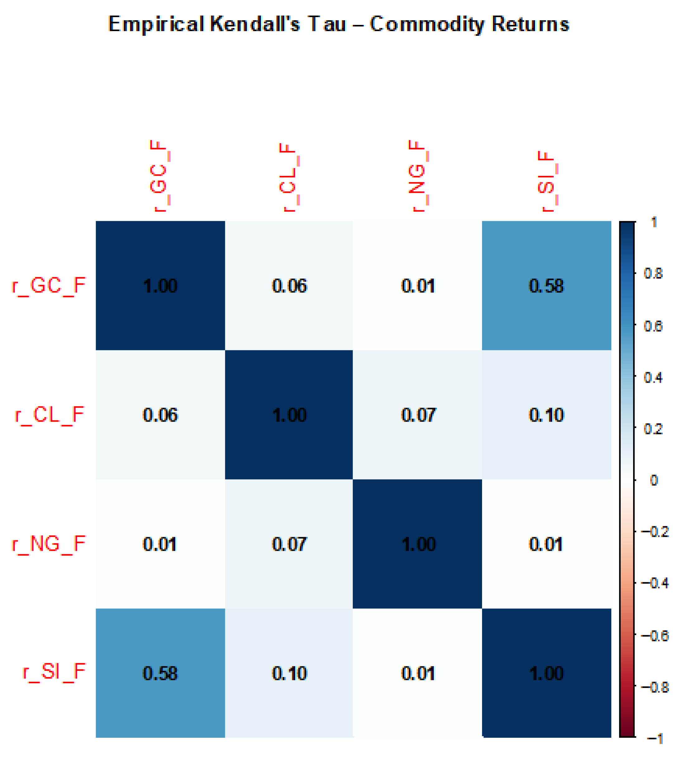
Figure 2 presents the Kendall’s τ coefficients for the daily returns of gold (GC), crude oil (CL), natural gas (NG), and silver (SI). The results indicate that dependence among commodity returns is generally weak, with most τ values close to zero. The strongest association appears between gold and silver (τ = 0.58), reflecting their shared role as precious metals and their tendency to co-move under similar macroeconomic or risk-aversion conditions. Energy assets exhibit minimal dependence. Oil–natural gas displays only a small positive association (τ = 0.07), suggesting independent short-term price dynamics despite their economic linkages. Gold shows no dependence with either oil (τ = 0.06) or natural gas (τ = 0.01), consistent with its behavior as a safe-haven asset that does not move in tandem with energy markets. Silver also exhibits weak correlations with oil (τ = 0.10) and natural gas (τ = 0.01), reinforcing the overall pattern of limited monotonic dependence across commodities. The conclusion is that linear or rank-based measures capture only modest co-movements. Therefore, one supports the use of vine copulas and tail-dependent models to uncover nonlinear or asymmetric relationships that do not surface in Kendall’s τ.

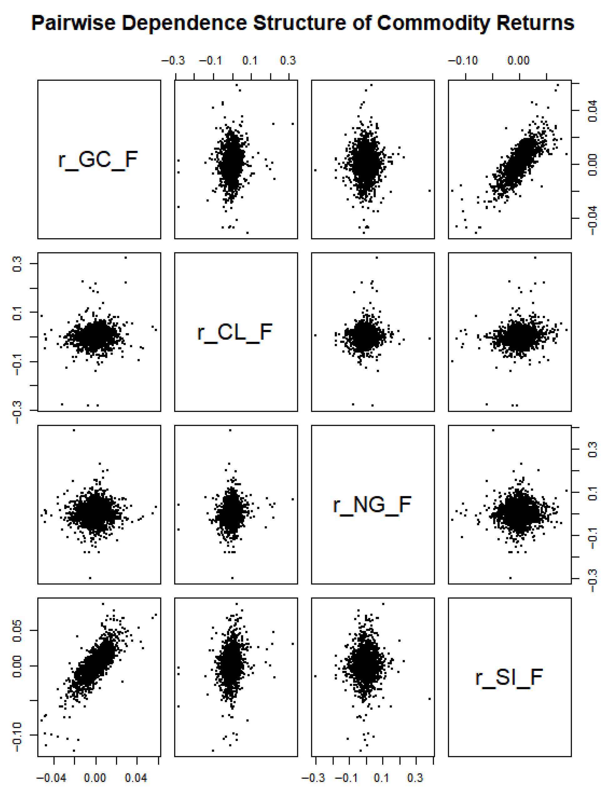
The notation ‘_F’ indicates the pseudo-observations obtained after applying the probability integral transform to the raw return series, which are the inputs used for estimating the vine copula model. The scatterplot matrix in Figure 3 confirms that most commodity pairs exhibit weak, nearly elliptical dependence, except for the stronger linear pattern between gold and silver, consistent with the Kendall’s τ matrix. It justifies the need for showing that linear co-movement is limited.

Table 11. CoVaR trapezoids for all commodity pairs.

α-Cut	GC–CL	GC–NG	GC–SI	CL–NG	CL–SI	NG–SI
10%	−0.05001805	−0.06589588	−0.07531959	−0.06841920	−0.03435960	−0.03241344
30%	−0.04863309	−0.06395247	−0.06747284	−0.06607091	−0.03295331	−0.03122500
70%	−0.04627582	−0.06139850	−0.05929208	−0.06378709	−0.03114862	−0.02844834
90%	−0.04477229	−0.06042549	−0.05313411	−0.06157978	−0.03041174	−0.02797960

reports the fuzzy CoVaR estimates for all commodity pairs across four α-cut levels (10%, 30%, 70%, 90%), where more negative values indicate stronger downside spillovers. Several patterns emerge. All CoVaR values are negative across all pairs and α-cuts, confirming that distress in one commodity consistently transmits downside risk to the other. Secondly, the strongest spillovers occur for gold–silver (GC–SI) and crude oil–natural gas (CL–NG), whose CoVaR intervals are the most negative (e.g., −0.0753 and −0.0684 at the 10% support level), indicating pronounced vulnerability in precious-metal co-movements and energy sector contagion. The weakest spillovers are observed for NG–SI and CL–SI, which display less negative CoVaR values, suggesting more muted cross-market transmission channels. As α increases from 10% to 90%, the CoVaR intervals become less negative, reflecting the movement from extreme but plausible stress scenarios (support) toward the most credible distress levels (core).

Table 12. Fuzzy lower tail dependence (λ_l) for all commodity pairs.

α-Cut	GC–CL	GC–NG	GC–SI	CL–NG	CL–SI	NG–SI
10%	0.02320841	0.00044327	0.2618516	0.07578108	0.01557847	0.00005901
30%	0.03493968	0.00062996	0.3205670	0.08766987	0.02357548	0.00087547
70%	0.04436035	0.00024935	0.3692199	0.10029102	0.03744885	0.00380174
90%	0.05557288	0.00089086	0.3884320	0.11124128	0.05459714	0.00715734

and

Table 13. Fuzzy upper tail dependence (λ_u) for all commodity pairs.

α-Cut	GC–CL	GC–NG	GC–SI	CL–NG	CL–SI	NG–SI
10%	0.02320841	0.00044327	0.2618516	0.00000000	0.01557847	0.00005901
30%	0.03493968	0.00062996	0.3205670	0.00000000	0.02357548	0.00087547
70%	0.04436035	0.00024935	0.3692199	0.00000000	0.03744885	0.00380174
90%	0.05557288	0.00089086	0.3884320	0.00000000	0.05459714	0.00715734

report the fuzzy lower- and upper-tail dependence coefficients for all commodity pairs. The results show that gold–silver (GC–SI) exhibits the strongest and most symmetric tail dependence, with λ values rising from approximately 0.26 to 0.39 across α-cuts, indicating that the two precious metals experience extreme gains and losses jointly. In contrast, crude oil–natural gas (CL–NG) displays lower-tail dominance; λ_l increases from 0.076 to 0.111, while λ_u remains zero at all α-levels. This asymmetry confirms that extreme negative shocks transmit strongly within the energy sector, whereas joint extreme gains are absent. The remaining pairs (GC–CL, CL–SI, NG–SI) show weak and symmetric tail dependence, suggesting limited co-movement under extreme conditions.

Table 14. Frequency of copula families in the asymmetric vine model.

Copula Code	Copula Family	Count	Type
0	Independence	20	Symmetric
2	Student-t	2	Symmetric
3	Clayton	1	Asymmetric
12	Rotated Clayton (180°)	1	Asymmetric

presents the frequency of copula families selected in the asymmetric vine model. The results show that the Independence copula dominates the structure (20 occurrences). Many conditional dependencies between commodity pairs are weak. The Student-t copula appears only twice, suggesting limited symmetric tail dependence in the system. In contrast, asymmetric copulas are selected only for two pairs (one Clayton and one 180° rotated Clayton), confirming that asymmetric tail behavior is present but rare. The vine structure is driven primarily by independence and symmetric copulas. Meaningful asymmetry arises only in isolated links, consistent with the finding that strong lower-tail dependence is concentrated in the crude oil–natural gas pair.

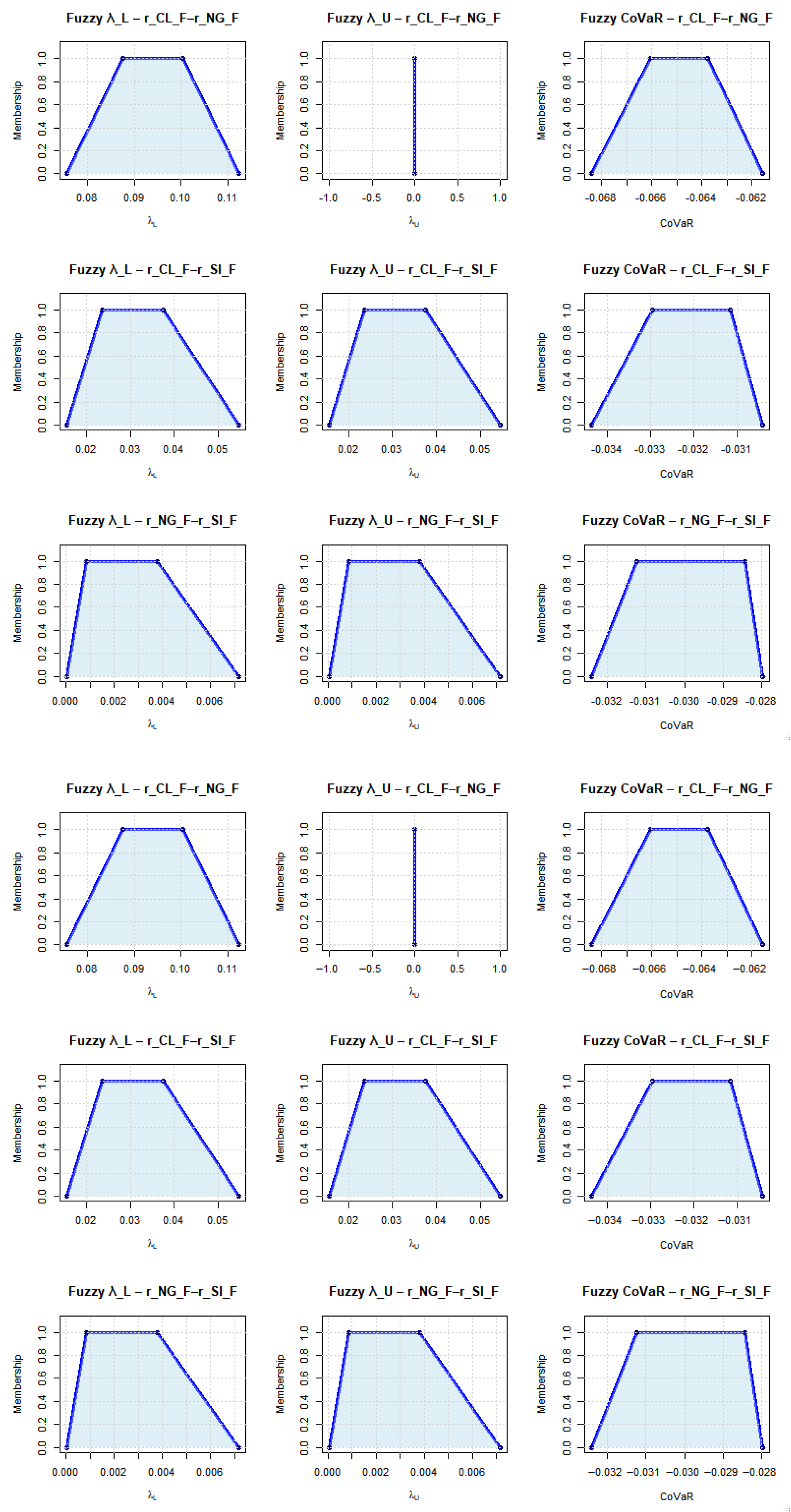
Figure 4 displays the TFNs obtained for the lower-tail dependence (λ_l), upper-tail dependence (λ_u), and CoVaR for selected commodity pairs. Each panel shows how the bootstrap distribution of the estimated risk measure is mapped into a fuzzy membership function. The central plateau (membership = 1) represents the most credible values, and the outer edges capture the full range of plausible outcomes under sampling uncertainty. For the CL–NG pair, the fuzzy lower-tail dependence exhibits a positive interval while the upper-tail dependence collapses to zero across the entire support, confirming pronounced lower-tail dominance, consistent with asymmetric contagion in energy markets. Pairs involving silver (CL–SI and NG–SI) display moderate but symmetric tail dependence, as reflected in nearly identical λ_l and λ_u trapezoids. The fuzzy CoVaR intervals are uniformly negative, indicating that distress in one commodity consistently transmits downside risk to the other. The width of each fuzzy trapezoid quantifies epistemic uncertainty; narrow supports indicate stable dependence estimates, whereas wider shapes signal parameter sensitivity arising from nonlinear dynamics and extreme events.

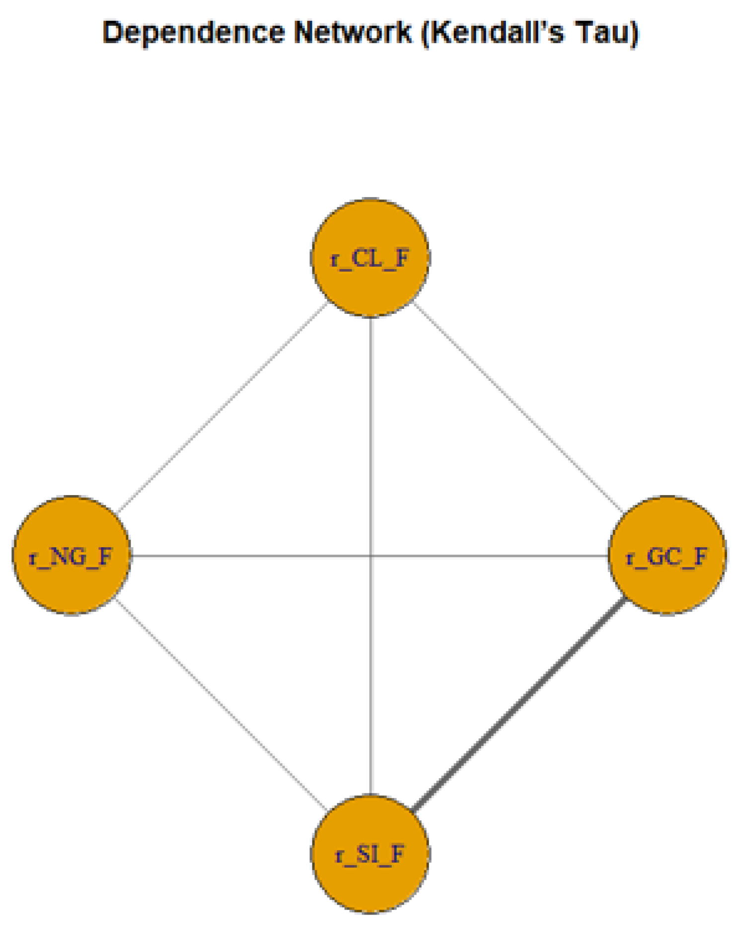
Figure 5 displays the dependence network constructed from the absolute values of Kendall’s τ for the four commodity returns. The network highlights the relative strength of pairwise associations through edge thickness, making the dependence structure visually transparent. The strongest connection in the system is the link between gold and silver (GC–SI), represented by the darkest and thickest edge, which confirms their well-known co-movement as precious metals driven by similar macroeconomic and financial factors. All other edges are noticeably thinner, reflecting only weak dependence between the remaining commodity pairs. The links involving natural gas (NG_F) are extremely light, indicating very limited monotonic association with the other commodities. The resulting network reveals a highly asymmetric topology: a tightly connected precious-metal cluster centered on silver, and a set of weakly linked energy–metal and energy–energy relationships. These findings reinforce the earlier Kendall’s τ results and justify the need for copula-based modeling to uncover nonlinear and tail-dependent relationships that are not captured by simple rank correlations.

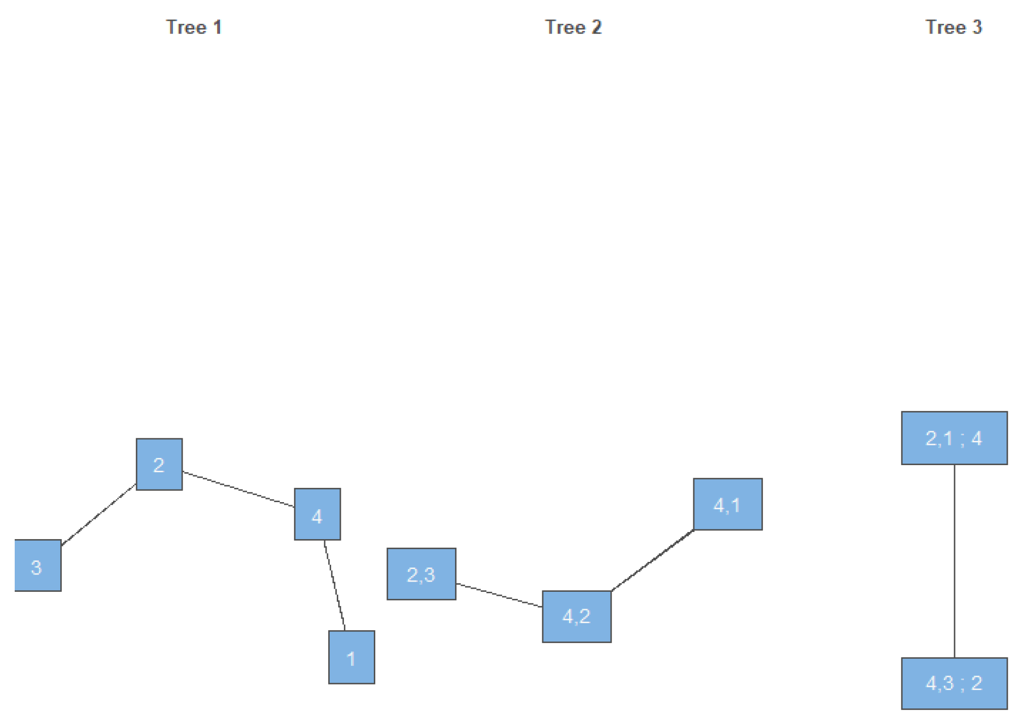
Figure 6 presents the selected vine structure for the commodity return series. Nodes 1–4 correspond to GC_F (gold), CL_F (crude oil), NG_F (natural gas), and SI_F (silver), respectively. In Tree 1, the primary unconditional dependence relationships appear; crude oil (node 2) is linked to silver (node 4), which in turn connects to gold (node 1), while natural gas (node 3) joins the system through crude oil. This indicates that silver serves as a bridge between oil and gold, and that natural gas enters the dependence structure only weakly through oil. In Tree 2, the model introduces conditional dependencies: the edge labeled “2,3,”, representing the dependence between crude oil and natural gas conditional on silver or gold. Additional edges like “4,2” and “4,1” show conditional connections involving silver and the other commodities. The reduction in the number of edges relative to Tree 1 reflects the fact that many dependencies weaken once conditioning is applied. Tree 3 shows only a single higher-order conditional relationship (e.g., “2,1;4” connected to “4,3;2”), meaning that very little dependence persists when conditioning on two variables simultaneously. The vine structure becomes progressively sparse from Tree 1 to Tree 3, confirming that most dependence among gold, oil, natural gas, and silver is either weak or disappears entirely under conditioning. This result is consistent with the dominance of Independence copulas in the final model.

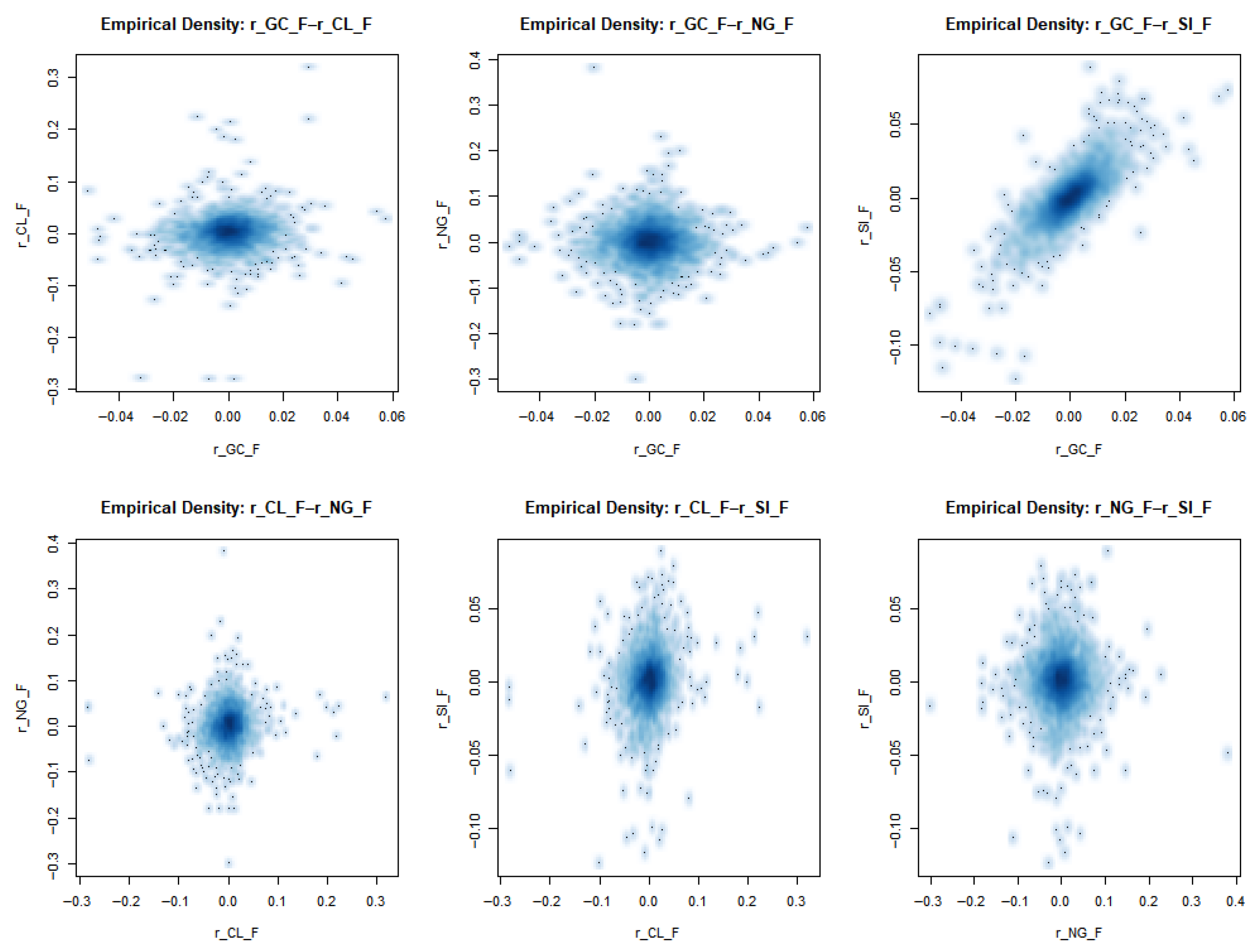
Figure 7 illustrates the empirical joint densities for all commodity pairs. Gold and silver show the strongest dependence, visible in the clearly elongated density cloud, while all pairs involving natural gas display nearly circular patterns, indicating very weak association. Gold–oil and oil–silver exhibit only mild dependence. The plots confirm that strong co-movement is limited to the precious metals, whereas energy commodities, especially natural gas, remain independent.

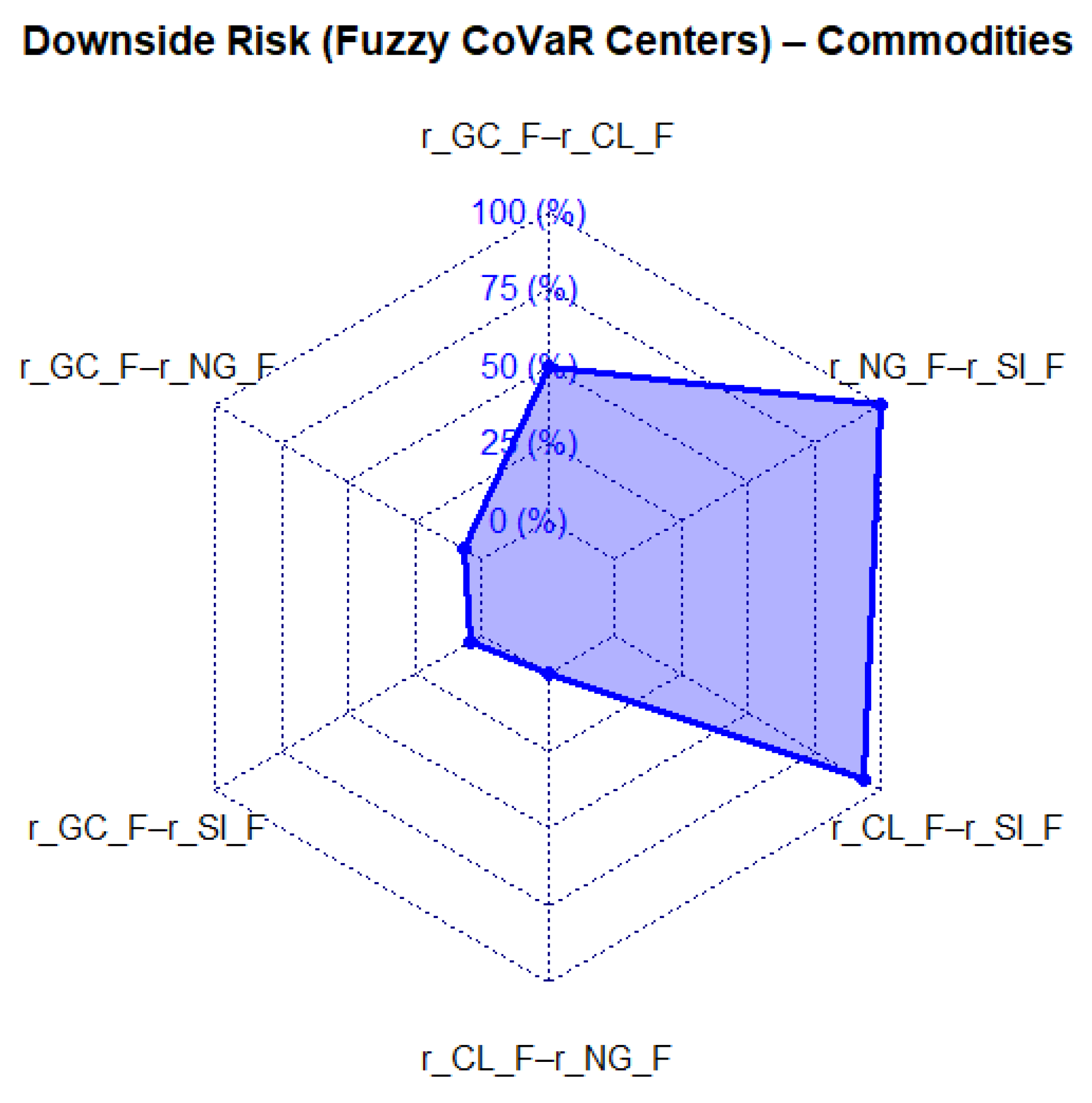
The radar chart in Figure 8 summarizes the central (most plausible) fuzzy CoVaR estimates for all commodity pairs, with larger values indicating stronger downside spillovers. The plot reveals that downside risk transmission is most pronounced for the CL–SI and NG–SI pairs, reflecting silver’s sensitivity to stress originating in both crude oil and natural gas. Gold-related pairs (GC–CL, GC–NG, GC–SI) show comparatively smaller CoVaR centers, indicating weaker spillover intensity. Figure 7 highlights silver’s central role in absorbing cross-commodity downside risk, while gold exhibits the lowest interconnectedness within the group.

5.2. Risk-Augmented Asymmetric Vine Copula Model with SKEW

Building on the baseline four-asset specification, this subsection introduces an asymmetric and risk-augmented five-asset vine copula model by incorporating SKEW as an additional variable to capture higher-order distributional asymmetries. The SKEW index, also extracted from Yahoo Finance, measures the perceived probability of extreme left-tail events in equity markets, capturing investors’ expectations of large downside risks and serving as a forward-looking indicator of aggregate market-implied tail-risk sentiment.

The asymmetric 5D vine in

Table 15. Comparison of symmetric versus asymmetric 5D vine copula models.

Model	LogLik	AIC	BIC
Symmetric 5D vine	1279.619	−2543.238	−2496.979
Full Asymmetric 5D vine	1281.343	−2546.687	−2500.428

shows a slightly higher log-likelihood and lower AIC/BIC than the symmetric vine, indicating only a small improvement in fit. This suggests that adding SKEW produces limited gains from modeling asymmetry. The dependence structure remains similar for the two specifications.

Adding SKEW to the model does not alter the copula-family selection for the original commodity pairs, discussed in Section 5.1. The asymmetric vine continues to be dominated by Independence and symmetric copulas, indicating that tail-risk expectations embedded in SKEW do not modify the underlying dependence structure of commodity markets.

Table 16. Summary of fuzzy tail dependence, asymmetry index, and CoVaR centers for all five-asset pairs.

Pair	λL (Center)	λU (Center)	Asymmetry Index (λL − λU)	CoVaR (Center)
GC–CL	0.04215	0.04215	0.00000	−0.04794
GC–NG	0.000296	0.000296	0.00000	−0.06225
GC–SI	0.35547	0.35547	0.00000	−0.06679
GC–SKEW	0.00000	0.00000	0.00000	−0.04103
CL–NG	0.09510	0.00000	0.09511	−0.06467
CL–SI	0.03252	0.03252	0.00000	−0.03216
CL–SKEW	0.00000	0.00000	−0.00000	−0.04107
NG–SI	0.00339	0.00339	0.00000	−0.03036
NG–SKEW	0.00000	0.00000	0.00000	−0.04129
SI–SKEW	0.00000	0.01764	−0.01764	−0.04142

Note: Bold values indicate asset pairs exhibiting asymmetric tail dependence (i.e., nonzero asymmetry index ∣λ_L − λ_U∣ > 0).

reports the fuzzy lower-tail dependence (λ_L), upper-tail dependence (λ_U), asymmetry index, and CoVaR centers for all pairs in the five-asset model that include SKEW. Several patterns emerge. Firstly, most pairs exhibit symmetric tail behavior, with λ_L = λ_U and asymmetry indices equal to zero. This confirms that adding SKEW does not introduce new asymmetric dependence for the majority of commodity pairs. The strongest tail dependence continues to be observed for gold–silver (GC–SI) and crude oil–natural gas (CL–NG), consistent with the baseline four-asset model.

Secondly, SKEW is tail-independent with all commodities. For GC–SKEW, CL–SKEW, NG–SKEW, and SI–SKEW, λ_L and λ_U are near zero, indicating no meaningful tail co-movement between equity-market tail-risk expectations (SKEW) and commodity returns. The only exception is SI–SKEW, which shows a small positive upper-tail dependence (λ_U = 0.01764), suggesting a very weak tendency for silver to co-move with periods of elevated right-tail equity-market skewness.

Thirdly, the CoVaR centers confirm that the strongest downside spillovers remain associated with gold–silver (−0.06679), GC–NG (−0.06225), and CL–NG (−0.06467), while all SKEW-related CoVaR values cluster around −0.041. This reflects a weak and uniform tail-risk impact from SKEW across commodities. It follows that adding SKEW to the model does not alter tail dependence or downside spillover patterns. Commodity tail dynamics remain mainly unchanged. SKEW behaves as a weakly connected, tail-independent variable.

Table 17. Fuzzy VaR trapezoids for all assets.

Asset	a	b	c	d
Gold (GC)	−0.07824	−0.06916	−0.05995	−0.05453
Crude Oil (CL)	−0.08350	−0.07240	−0.06492	−0.05877
Natural Gas (NG)	−0.10247	−0.08563	−0.07290	−0.06610
Silver (SI)	−0.08977	−0.07602	−0.06685	−0.06014
SKEW Index	−0.01182	−0.00657	−0.00411	−0.00262

reports the fuzzy VaR trapezoids at the 95% confidence level for all assets. Each trapezoid is defined by four parameters (a, b, c, d), representing increasing degrees of plausibility for the asset’s downside loss. Among all commodities, the fuzzy VaR bounds are negative, indicating potential losses under adverse market conditions.

Among the commodities, natural gas exhibits the largest downside risk, with its trapezoid spanning from −0.10247 to −0.06610. This reflects the high volatility and pronounced tail behavior characteristic of natural gas markets (Ding 2021; Sæther and Neumann 2025). Crude oil and silver follow, showing moderately large VaR values. Gold displays the smallest downside risk among the commodities, consistent with its role as a relatively stable safe-haven asset.

The SKEW index shows a much smaller range of negative values (from −0.01182 to −0.00262), confirming that it does not behave like a traded asset and exhibits minimal price variability. Its narrow trapezoid indicates low volatility and limited downside fluctuation compared with physical commodities.

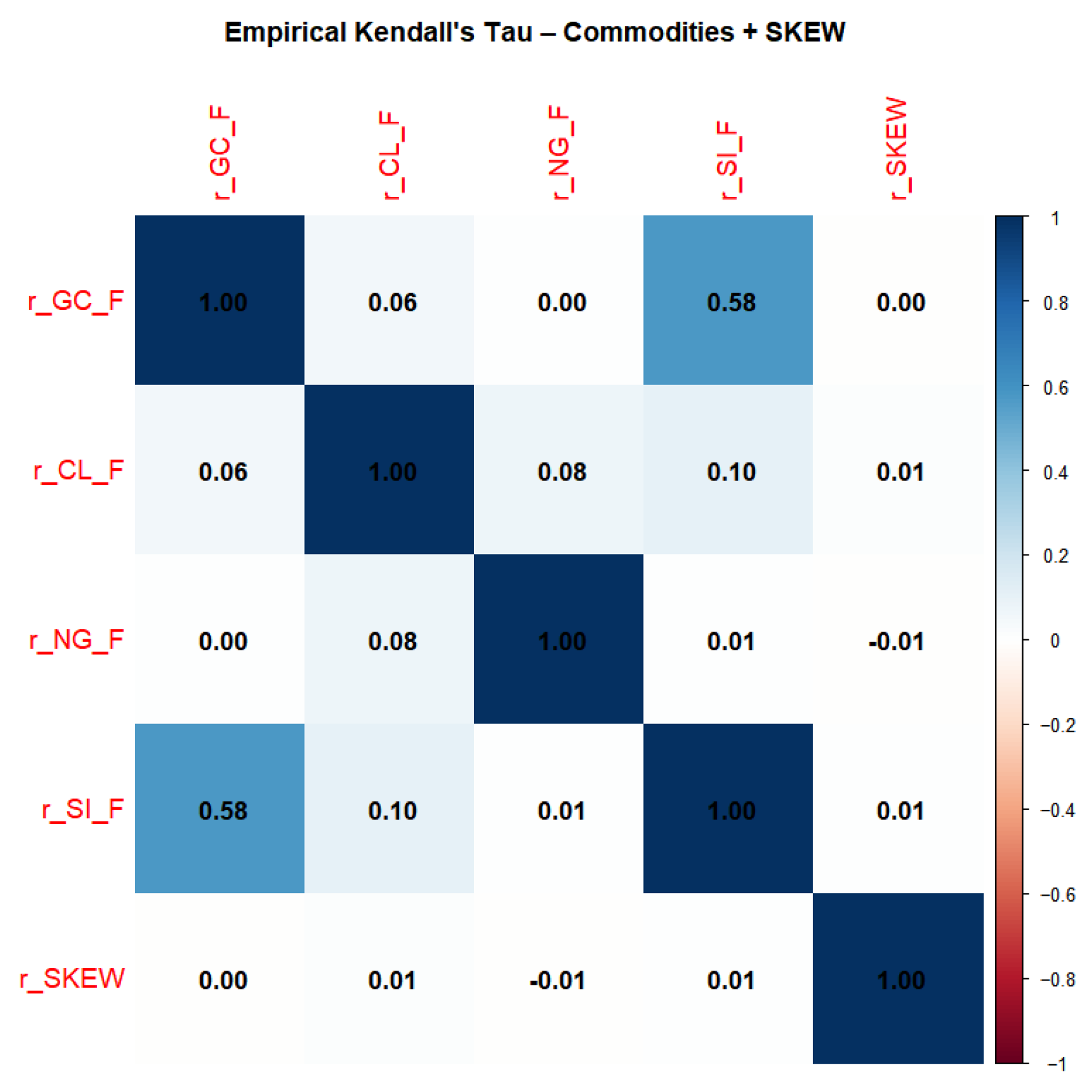
Figure 9 presents Kendall’s τ dependence matrix for gold (GC), crude oil (CL), natural gas (NG), silver (SI), and the SKEW index. The strongest dependence occurs between gold and silver (τ = 0.58), consistent with their shared role as precious metals. All other commodity pairs exhibit very weak dependence, with τ values near zero, including GC–CL (0.06), CL–NG (0.08), and CL–SI (0.10).

SKEW shows almost no dependence on any commodity, with τ values effectively equal to zero across all pairs. This indicates that equity-market tail-risk expectations embedded in SKEW do not translate into meaningful co-movements with daily commodity returns.

The matrix highlights a highly sparse dependence structure, dominated by the gold–silver relationship, while both energy commodities and SKEW remain independent.

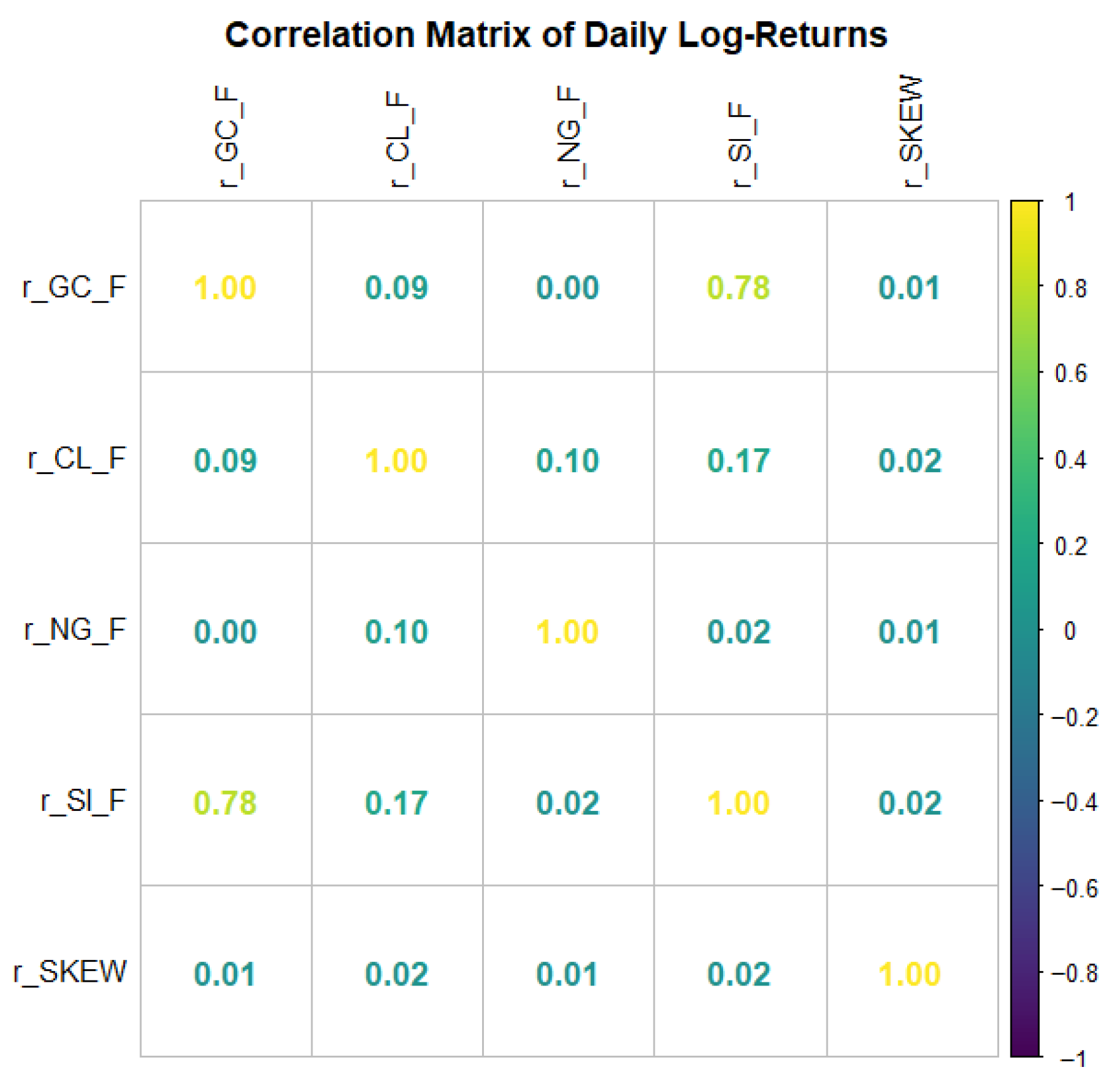
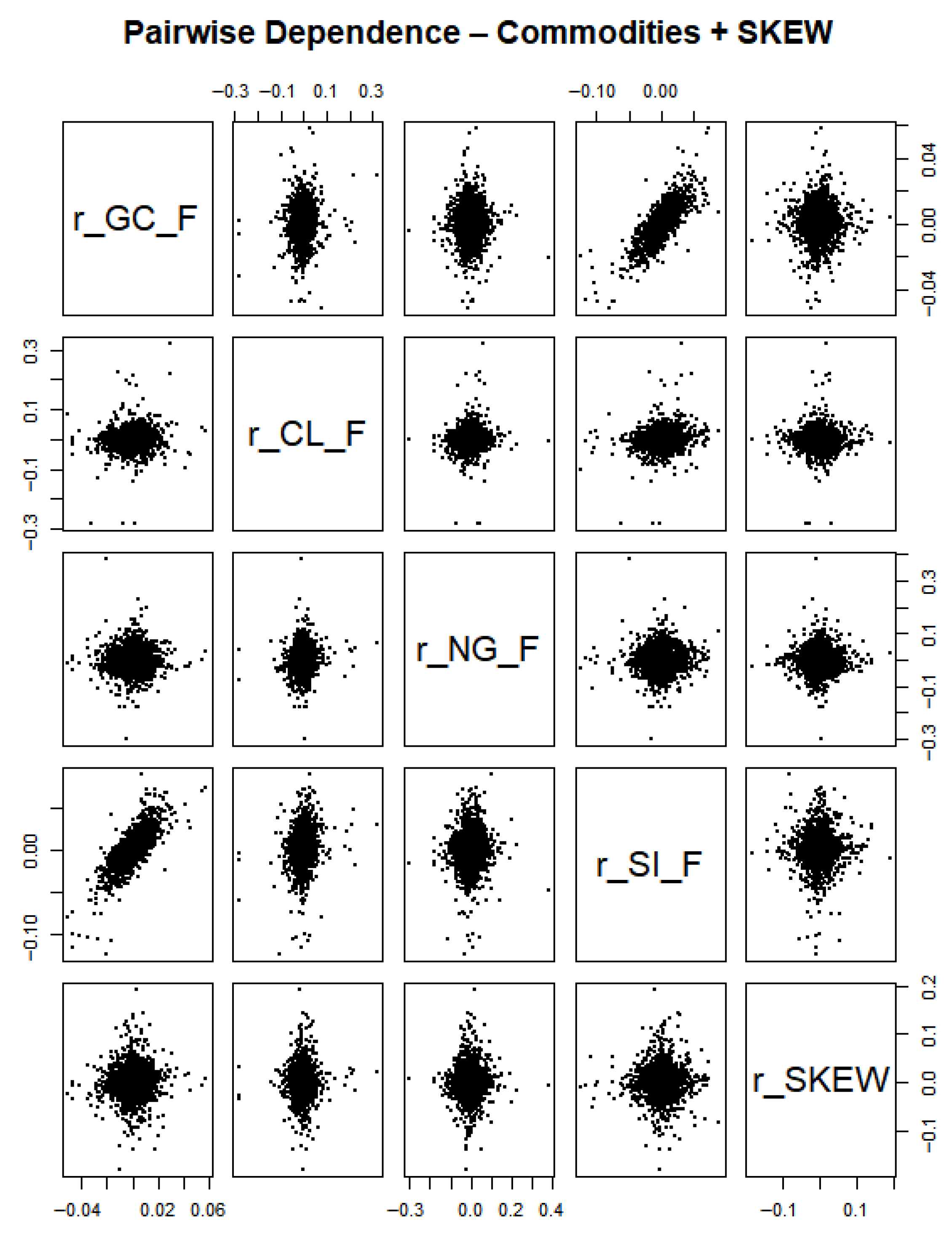
The scatterplot matrix in Figure 10 visualizes the bivariate dependence structure among the five variables (GC, CL, NG, SI, and SKEW). Consistent with Kendall’s τ matrix, the only visibly strong relationship is between gold and silver, which shows a positive, elongated cloud of points indicating meaningful co-movement. All other commodity pairs display highly diffuse, nearly circular scatter patterns, indicating weak or negligible dependence—particularly for natural gas, which shows no strong association with any other asset.

Panels involving SKEW show completely unstructured point clouds with no directional pattern, confirming that SKEW is essentially independent of commodity returns in the sample.

Figure 10 highlights a highly sparse dependence network, with strong co-movement confined to the precious metals, while energy commodities and SKEW remain uncorrelated.

Table 18. Fuzzy CoVaR trapezoids for all commodity and SKEW pairs.

Fuzzy Level	GC–CL	GC–NG	GC–SI	GC–SKEW	CL–NG	CL–SI	CL–SKEW	NG–SI	NG–SKEW	SI–SKEW
10%	−0.05004	−0.06506	−0.07490	−0.04233	−0.06807	−0.03427	−0.04137	−0.03261	−0.04252	−0.04132
30%	−0.04908	−0.06369	−0.07291	−0.04173	−0.06359	−0.03212	−0.04180	−0.03130	−0.04190	−0.04213
70%	−0.04680	−0.06801	−0.06606	−0.04033	−0.06350	−0.03115	−0.04034	−0.02926	−0.04068	−0.04077
90%	−0.04440	−0.05949	−0.05928	−0.03950	−0.05986	−0.03032	−0.03956	−0.02735	−0.03986	−0.03969

reports the fuzzy CoVaR trapezoids at different α-cuts for all commodity–commodity and commodity–SKEW pairs. The trapezoid centers (increasing from 10% to 90%) remain negative, indicating that distress in one asset systematically increases downside risk in the other. The magnitude of CoVaR varies substantially across pairs.

The largest downside spillovers occur for the pairs GC–NG, GC–SI, and CL–NG, with CoVaR values of around −0.06 to −0.075 at low α-cuts. These values indicate that shocks in natural gas and silver generate the strongest downside risk transmission to other markets.

Pairs involving SKEW produce moderate and uniform CoVaR values around −0.04 across all α-cuts, showing that tail-risk expectations embedded in SKEW transmit only weak and uniform downside effects. The effect is much weaker than for direct commodity interactions. The relatively narrow trapezoids for SKEW pairs suggest low uncertainty and stable spillover patterns.

The smallest spillovers appear in NG–SI and CL–SI, which exhibit CoVaR values closer to −0.03, indicating limited contagion between these commodities.

Table 19. Fuzzy lower-tail dependence (λ_L) for all commodity–SKEW pairs.

Fuzzy Level	GC–CL	GC–NG	GC–SI	GC–SKEW	CL–NG	CL–SI	CL–SKEW	NG–SI	NG–SKEW	SI–SKEW
10%	0.01840	4.89 × 10−6	0.29244	0	0.07838	0.01664	0	6.43 × 10−5	0	0
30%	0.03545	1.73 × 10−5	0.33167	0	0.08535	0.02363	0	6.97 × 10−4	0	0
70%	0.04886	5.75 × 10−4	0.37965	0	0.10486	0.04412	0	6.09 × 10−3	0	0
90%	0.05754	1.82 × 10−3	0.40839	0	0.11679	0.05138	0	1.22 × 10−2	0	0

and

Table 20. Fuzzy upper-tail dependence (λ_U) for all commodity–SKEW pairs.

Fuzzy Level	GC–CL	GC–NG	GC–SI	GC–SKEW	CL–NG	CL–SI	CL–SKEW	NG–SI	NG–SKEW	SI–SKEW
10%	0.01840	4.89 × 10−6	0.29244	0	0.00000	0.01664	0	6.43 × 10−5	0	0.000080
30%	0.03545	1.72 × 10−5	0.33167	0	0.00000	0.02363	0	6.97 × 10−4	0	0.01000
70%	0.04886	5.75 × 10−4	0.37965	0	0.04142	0.04412	0	6.09 × 10−3	0	0.02300
90%	0.05754	1.82 × 10−3	0.40839	0	0.05138	0.05138	0	1.22 × 10−2	0	0.03466

summarize the fuzzy lower-tail (λ_L) and upper-tail (λ_U) dependence estimates for all commodity–commodity and commodity–SKEW pairs. The strongest tail dependence arises in the gold–silver (GC–SI) and crude oil–natural gas (CL–NG) pairs, whose λ-values increase steadily with the α-cut. Precious metals are tightly linked in both downside and upside market conditions. Energy commodities exhibit a similarly pronounced co-movement structure. For most other commodity pairs, tail dependence remains weak and symmetric, as indicated by the λ_L and λ_U values, which are nearly identical across all fuzzy levels. This suggests that joint crashes and joint booms occur with comparable intensity among the weaker pairs, and there is no systematic directional asymmetry in their tail behavior.

An exception is the CL–NG pair at lower α-cuts, where λ_L is positive while λ_U equals zero. This pattern indicates a form of downside contagion within the energy sector; crude oil and natural gas tend to co-crash more intensely than they co-boom, although this asymmetry diminishes at higher fuzzy levels where λ_U becomes positive. The NG–SI pair displays only marginal and gradually increasing tail dependence, consistent with a very weak but slightly strengthening connection between natural gas and silver.

SKEW exhibits no lower-tail dependence with any of the commodities, as λ_L equals zero for all SKEW-related pairs. Equity-market tail-risk expectations do not synchronize with downside movements in commodity markets. Upper-tail dependence is also negligible for SKEW, with the only detectable link being a very small positive λ_U between SKEW and silver. This weak upper-tail co-movement suggests that, at most, silver may respond marginally to periods of elevated right-tail risk in equity markets, although the magnitude is insignificant.

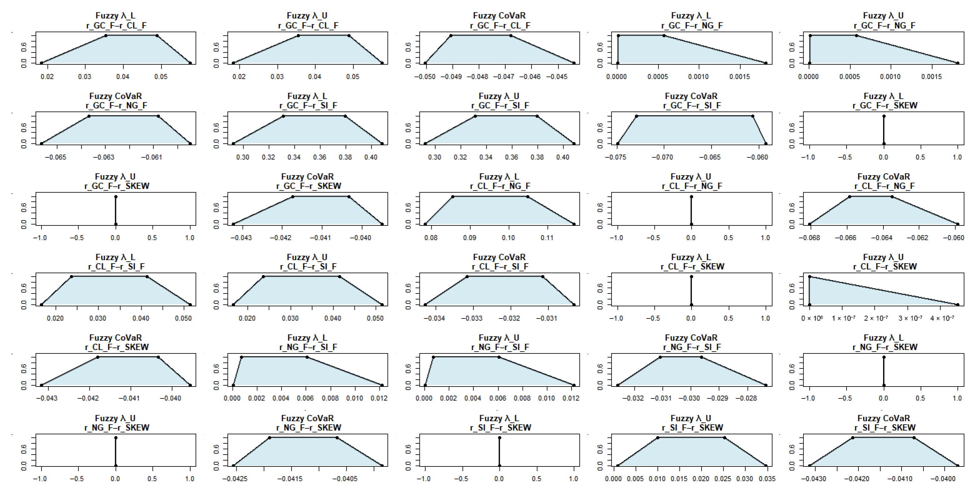
Figure 11 displays the fuzzy trapezoids for lower-tail dependence (λ_L), upper-tail dependence (λ_U), and CoVaR for every pair in the five-asset system. The shapes show that most commodity pairs have symmetric tail behavior, with nearly identical λ_L and λ_U regions. Stronger fuzzy tail dependence appears for GC–SI and CL–NG, while all pairs involving SKEW exhibit flat or near-zero trapezoids, indicating negligible tail co-movement with market-implied tail-risk expectations. The CoVaR trapezoids confirm that downside risk spillovers remain concentrated among the commodities themselves, whereas SKEW contributes only minimal additional tail-risk effects.

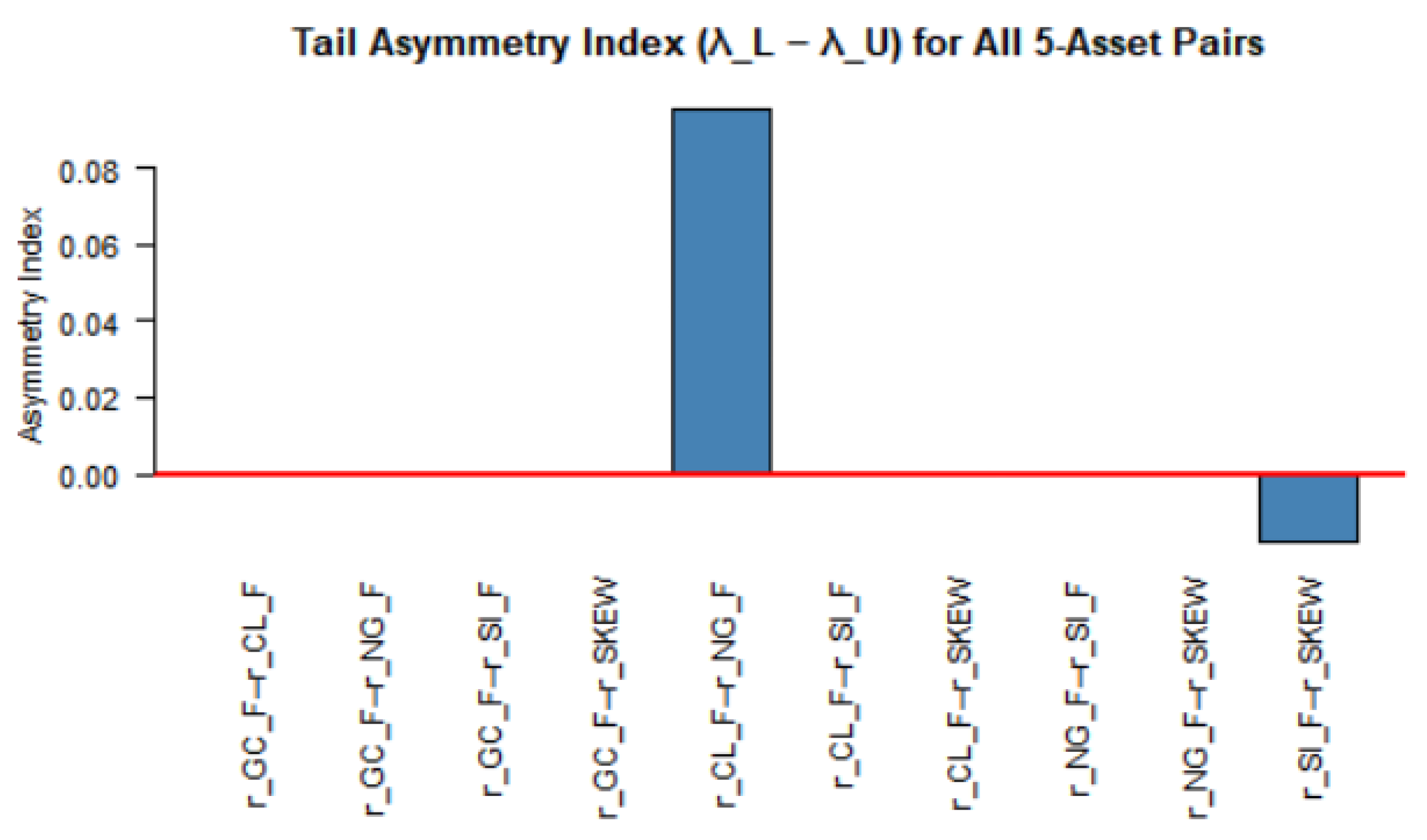
Figure 12 displays the tail asymmetry index. A positive value indicates stronger co-movement during extreme downturns than during upturns, while a negative value signals stronger upper-tail dependence. Crude oil–natural gas (CL–NG) is the only pair exhibiting notable positive asymmetry; λ_l exceeds λ_u by nearly 0.10. This confirms that downside contagion is significantly stronger than upside co-movement within the energy sector, meaning that oil and natural gas tend to co-crash more severely than they co-boom.

All other commodity and SKEW pairs display asymmetry indices very close to zero, indicating symmetric tail behavior. The only slight negative value appears in silver–SKEW (SI–SKEW), suggesting a minimal tendency for silver to exhibit slightly stronger upper-tail than lower-tail co-movement with equity-market skewness—though the magnitude is economically negligible.

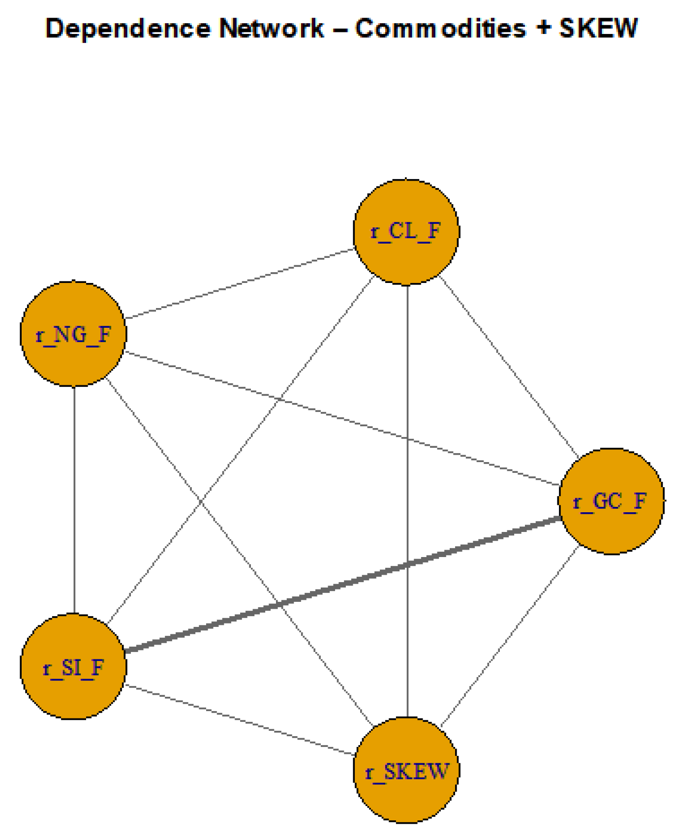
The network in Figure 13 visualizes the strength of pairwise dependence among the four commodities and the SKEW index. The thickest edge appears between gold and silver, highlighting the strongest linkage in the system. All other edges are thin, indicating weak dependence across commodities and especially between SKEW and all commodity returns. This confirms that adding SKEW does not alter the dependence structure, as market-implied tail-risk expectations display minimal direct connection with commodity markets.

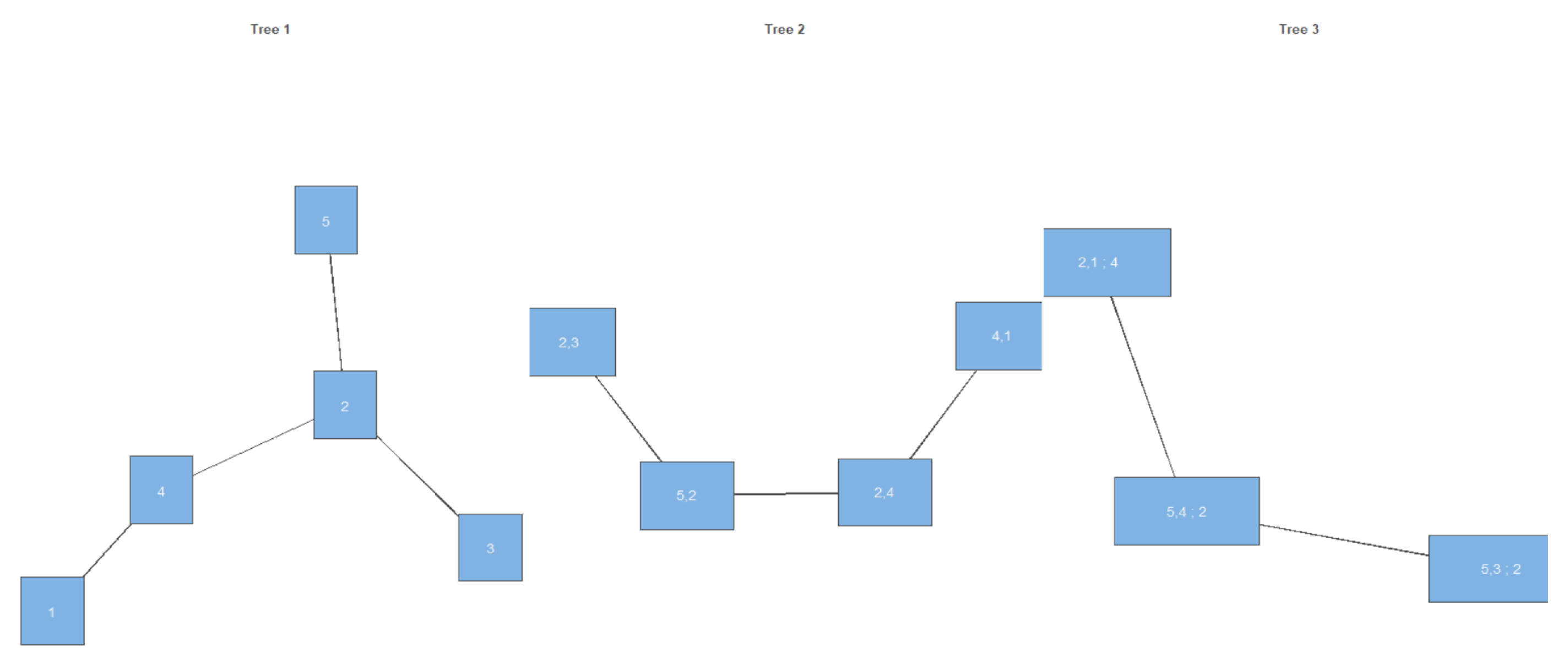
The five-asset vine in Figure 14 reveals that the core dependence structure among the four commodities (gold, oil, natural gas, and silver) remains unchanged after including SKEW. In Tree 1, the main chain continues to run through oil (node 2), linking silver, natural gas, and gold, while SKEW (node 5) attaches only weakly to the system. Trees 2 and 3 show sparse conditional dependencies, with higher-order links becoming progressively weaker. The vine confirms that SKEW plays a peripheral role, contributing little to the dependence structure. Commodity–commodity linkages dominate, in line with the fuzzy tail-dependence and CoVaR results.

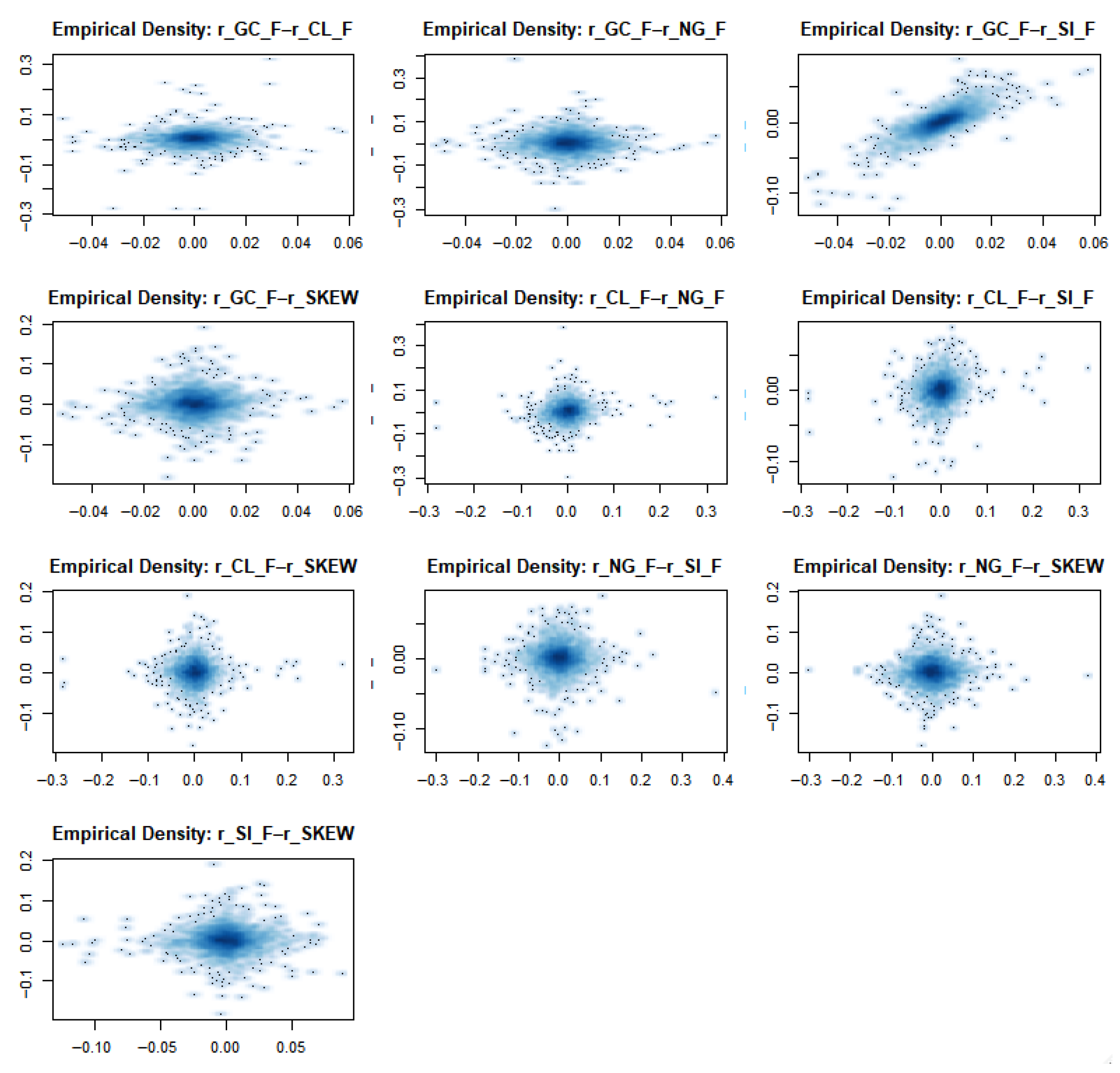
The empirical densities in Figure 15 show that gold–silver remains the only pair with visibly strong co-movement. All other commodity pairs display weak, diffuse dependence structures. Every plot involving SKEW exhibits an almost circular density cloud, indicating minimal or no dependence between equity-market tail-risk expectations and commodity returns. This visual evidence reinforces the earlier results from Kendall’s τ and the vine copula models; SKEW does not influence the dependence structure of commodity markets.

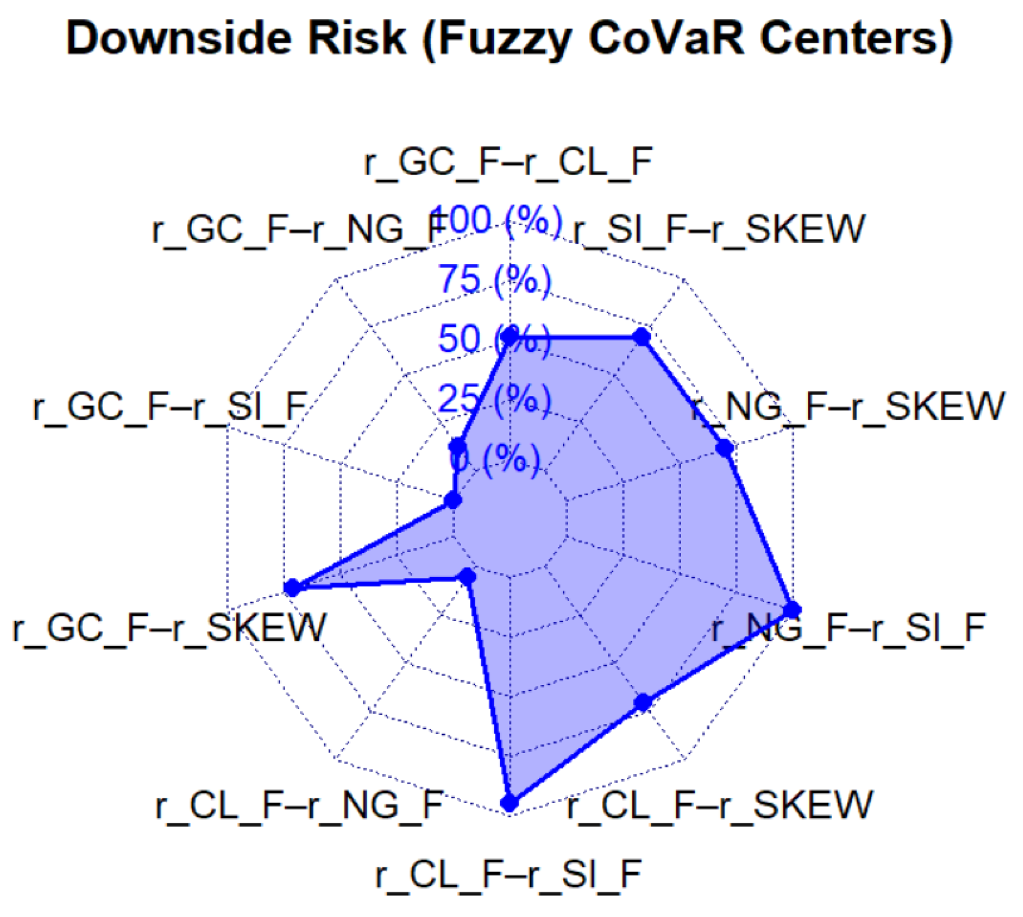
The radar plot in Figure 16 illustrates the central fuzzy CoVaR values for all commodity–commodity and commodity–SKEW pairs. The strongest downside spillovers arise from energy-to-precious-metals links, particularly natural gas and crude oil toward silver. Gold shows only moderate spillover sensitivity. All SKEW-related pairs appear close to the plot’s center, indicating that equity-market tail-risk expectations captured by SKEW exert minimal direct spillover effects on commodity returns. Risk transmission occurs mainly within the commodity complex, with SKEW playing only a peripheral role.

Market-wide tail risk in this study is proxied by the SKEW index, and the weak transmission effects should not be viewed as a limitation. Rather, they highlight a structural distinction between equity-market tail-risk expectations and physical commodity market dynamics. The SKEW index captures sentiment-driven, option-implied equity tail risk, whereas commodity prices—particularly in energy and raw materials—are mainly shaped by sector-specific fundamentals such as supply constraints, inventories, geopolitical disruptions (Kinnunen et al. 2024), and regulation. Consequently, the limited spillover from SKEW indicates a segmented risk transmission mechanism, operating through real-economy and sectoral channels rather than generalized financial sentiment. This segmentation represents a novel insight, suggesting that commodity risk dynamics cannot be fully inferred from equity-based tail-risk measures.

The dominance of Independence copulas in the vine structure indicates that dependence across many commodity pairs is weak or episodic rather than persistent. Economically, this suggests that common shocks do not systematically propagate across the entire system, preserving diversification benefits under normal market conditions. Dependence intensifies only for specific pairs and periods, consistent with the observed localized nature of systemic risk.

6. Static Versus Regime-Dependent Dependence Structure

The present analysis was conducted over a full sample of the period 1 January 2015–1 January 2025 and does not explicitly model time variation or regime shifts in the dependence structure. This modeling choice is consistent with the main objective of this study, namely to characterize distributional dependence and tail behavior rather than temporal dynamics.

Vine copula models, in their standard static formulation, are designed to reflect complex nonlinear dependence patterns, including asymmetric dependence and heterogeneous pairwise comparisons (Czado 2019; Czado and Nagler 2022). The estimated dependence should therefore be interpreted as an average representation over the sample period rather than a sequence of time-localized regimes.

The use of a bootstrap-based fuzzy framework partially mitigates the absence of regime modeling. By introducing parameter uncertainty and widening dependence supports in tails, the bootstrap absorbs latent instability derived from regime changes or episodic market stress. Similar studies by Gneiting and Katzfuss (2014) argue that including epistemic risk and distributional uncertainty into dependence modeling can partially reflect structural instability, in the absence of regime-dependent parameters.

Compared to classical (non-fuzzy) inference, which relies on crisp parameter estimates and fixed dependence classification, the fuzzy framework allows for gradual transitions and partial membership across dependence regimes. While classical inference provides a single static representation of dependence, fuzzy inference includes parameter uncertainty, yielding more robust and informative assessments under latent regime instability. This feature is relevant in commodity and financial markets, where dependence structures evolve smoothly rather than through abrupt regime shifts.

The literature has distinguished between static and dynamic dependence models. The static dependence models focus on structural relationships in the joint distribution. Dynamic dependence models focus on temporal evolution (Creal and Tsay 2015). Time-varying vine copulas and regime-switching copulas have been proposed to capture evolving dependence (Vatter and Nagler 2018). These approaches require longer samples, higher computational complexity, and strong assumptions on regime persistence and transition.

7. Conclusions

This study combined fuzzy tail-risk and spillover measures with asymmetric vine copulas to assess dependence and spillover risk in commodity markets, with and without the SKEW index. The results show that commodity markets exhibit weak overall dependence, with gold–silver as the only consistently strong link. Asymmetric tail effects are limited and appear mainly in the crude oil–natural gas pair, indicating downside-driven contagion within the energy sector.

Fuzzy CoVaR confirms that downside spillovers are concentrated in a small set of commodity pairs. SKEW contributes minimal additional dependence or tail risk, acting as a weakly connected variable. Thus, risk transmission in commodity markets arises primarily from within-market interactions, rather than from broader equity-market tail-risk sentiment.

The findings indicate that risk transmission in commodity markets is highly localized, with the strongest transmission occurring within the energy sector and the precious-metals cluster. Policymakers and market regulators should therefore monitor oil–natural gas and gold–silver linkages more closely, especially during periods of market stress. Since SKEW plays only a marginal role, spillovers from equity-market tail-risk sentiment into commodities appear limited, supporting a more sector-specific monitoring strategy rather than broad cross-market interventions. Enhanced transparency in energy markets and improved hedging instruments may further mitigate downside contagion within the commodity system.

The absence of strong SKEW spillovers suggests a segmentation between equity-market tail-risk expectations and physical commodity price formation. This result reinforces the view that commodity risk dynamics are mainly sector-specific and driven by economic and supply-side factors rather than by sentiment-driven financial risk.

The results suggest that commodity risk management should focus on sector-specific tail-risk linkages rather than broad market indicators. Strong downside dependence within the energy sector, particularly between crude oil and natural gas, implies that diversification across closely related commodities may fail during stress periods. Managers should therefore complement standard risk measures with tail-sensitive tools, such as fuzzy CoVaR, to better capture extreme risk transmission.

For investors, the weak spillover role of SKEW indicates that commodity markets remain partially insulated from equity-market tail-risk sentiment. Strong within-sector tail dependence exposes portfolios to localized systemic risk, especially in energy and precious metals. Dynamic hedging and portfolio strategies that account for asymmetric tail dependence are therefore essential for downside risk management.

From a policy perspective, the findings support a targeted regulatory approach to systemic risk in commodity markets. Since tail-risk spillovers are concentrated in specific commodity pairs, regulators should prioritize monitoring main relationships, such as oil–natural gas and gold–silver, rather than broad cross-market interventions. Improved market transparency and sector-specific oversight may further reduce downside contagion during periods of stress.

This study has several limitations that could be explored in future work. Firstly, the analysis relies on daily data, which may miss intraday contagion patterns. Extending the model to high-frequency or regime-switching settings could refine tail-risk and spillover detection. Secondly, the empirical analysis focuses on a limited set of strategically important commodities, reducing the generalizability of the findings. The selected commodities representing energy and precious metals are among the most liquid, globally traded, and studied assets, being benchmarks for market complexity and nonlinear dependence. The proposed methodological framework can be extended to a broader range, including agricultural products and industrial metals. Thirdly, while SKEW was included as a market-implied tail-risk proxy, other macro-financial indicators, such as VIX, geopolitical risk, or climate-related shocks, may reveal broader transmission channels. Fourthly, the fuzzy and vine copula framework, although flexible, remains computationally intensive for larger portfolios, suggesting the need for scalable or machine-learning-based dependence models.