A Convergent Collocation Approach for Generalized Fractional Integro-Differential Equations Using Jacobi Poly-Fractonomials

Abstract

In this paper, we present a convergent collocation method with which to find the numerical solution of a generalized fractional integro-differential equation (GFIDE). The presented approach is based on the collocation method using Jacobi poly-fractonomials. The GFIDE is defined in terms of the B-operator introduced recently, and it reduces to Caputo fractional derivative and other fractional derivatives in special cases. The convergence and error analysis of the proposed method are also established. Linear and nonlinear cases of the considered GFIDEs are numerically solved and simulation results are presented to validate the theoretical results.

1. Introduction

Fractional calculus is the branch of applied mathematics in which we deal with integration and differentiation of arbitrary order [1,2,3,4,5,6,7]. Fractional-order derivatives and integrations arise in the modeling of several problems in various domains including physics, engineering, and biology. In the last few decades, applications of fractional differential equations (FDEs) have increased very rapidly in different fields like bioengineering [8], fluid dynamics [9], electrochemistry [10], electromagnetism [11], Control theory [12], and viscoelasticity [13]. Introductory overview of fractional order derivatives and recent developments are presented in [1]. In recent years, fractional integro-differential equations (FIDEs) have been investigated to represent the physical phenomena in various fields such as electromagnetics [14]. Several researchers have been concentrating on the development of numerical and analytical techniques for FIDEs. For example, Angell and Olmstead [15] solved integro-differential equation modeling filament stretching using by Singular perturbation method. Khosro et al. [16] presented a numerical technique based on Bernstein’s operational matrix for a family of FIDEs utilizing the trapezoidal rule. Kilbas et al. [17] developed some basic concepts for solving FIDEs, and also provided the existence and uniqueness theorem. In [18], a new set of functions was constructed to obtain the numerical solution of FIDEs, called the fractional-order Euler function, which is based on the Euler function. By using the property of the fractional-order Euler function, the authors found the approximate solution using the operational matrix approach, and also discussed the convergence analysis of the problem. Saddatmandi and Dehghan [19] developed a numerical method for solving linear and nonlinear FIDEs by defining the fractional derivative in the Caputo sense. The approximate solution was found by Legendre approximations. The property of Legendre polynomials together with the Gaussian integration method were utilized to convert the system of algebraic equations. In [20], two numerical approximations for the generalized Abel integral were proposed, and a generalized Abel integral equation was solved by two numerical schemes, i.e., linear and quadratic. The error and convergence were also discussed. It was found that the quadratic scheme achieved a convergence order up to three. Bonilla et al. [21] dealt with the linear system of the fractional differential equation defined in the form of the Riemann-Liouville or Caputo fractional derivative. In [22,23], Adomian’s decomposition method for solving the system of the nonlinear FIDEs was discussed. In [24,25,26,27,28,29], the authors used the collocation method for solving the fractional differential equations. Odibat [30] presented the analytical study on a linear system of fractional differential equations with constant coefficient and briefly described the issue of the existence and uniqueness of systems of fractional order differential equations. There are many more methods to solve FIDEs, such as the Finite difference method and Finite-element methods [31]. Kamal et al. [32] applied the spectral Tau method to solve general fractional-order differential equations. In [33], a system of fractional differential equations was solved by the homotopy analysis method. Some recent work in this field was done by Hassani et al. [34]. The authors proposed a method for solving a system of nonlinear fractional-order partial differential equations with initial conditions. First, they expanded the solution by using the operational matrix method, and then the unknown coefficients were evaluated by the optimization technique.

Here, we consider the GFIDEs in terms of the B-operator [35]. The B-operator reduces to Caputo derivative and Riemann Liouville derivative for a particular choice of kernel in B-operator. The GFIDEs are solved using the collocation method with Jacobi poly-fractonomials. The details of the Jacobi poly-fractonomials are presented in [36]. It has been noted that Jacobi poly-fractonomials, as basis functions, have an edge over the other known standard polynomials, as the method achieves exponential convergence in approximating fractional polynomial functions. The GFIDEs converted into a system of algebraic equations and, by solving them we get the approximate solution of the GFIDEs. The main aim of this study is to investigate an approximate method with higher accuracy in finding the approximate solution of defined GFIDEs, which is close to the exact solution. Section 1 provides the basic definitions of the operator as given in [35], including some basic properties of Jacobi poly-fractonomials [36].

The rest of the paper is organized as follows: Section 2 provides the procedure to apply Collocation methods for solving GFIDEs. Section 3 provides a convergence analysis of the method. In Section 4, we present an error analysis in two parts, by taking linear and nonlinear cases of the GFIDEs. Section 5 presents five numerical examples that illustrate the accuracy of the proposed method. Finally in Section 6, a conclusion is presented.

1.1. Generalized Fractional Integro-Differential Equations

We first define GFIDEs in terms of K and A/B-operators. These operators [35] are defined as follows:

$$K^{\alpha }{}_{P}f\left(x\right)=r{{\displaystyle \int }}_a^x{w}_{\alpha }\left(x,t\right)f\left(t\right)dt+s{{\displaystyle \int }}_x^b{w}_{\alpha }\left(t,x\right)f\left(t\right)dt ,\alpha >0,$$

(1)

where $x\in \left[a,b\right] , P=⟨a,x,b,r,s⟩$ denote the all parameters, $w_{\alpha }\left(x,t\right)$ is a kernel defined on the space $I\times I.$ we assume that $w_{\alpha }\left(x,t\right)$ and f(t) both are square integrable function such that Equation (1) exists. K operator satisfies the linearity properties, i.e., for any two functions $f_1\left(t\right)$ and $f_2\left(t\right)$, then

$$K_P^{\alpha } \left(f_1\left(x\right)+f\left(x\right)\right)=K^{\alpha }{}_P{f}_1\left(x\right)+K^{\alpha }{}_P{f}_2\left(x\right) .$$

(2)

Define A and B-operators [35] as follows,

$$A_P^{\alpha }f\left(x\right)={\mathfrak{D}}^n{K}^{n-\alpha }{}_{P}f\left(x\right),$$

(3)

$$B_P^{\alpha }f\left(x\right)=K^{n-\alpha }{}_P{\mathfrak{D}}^{n}f\left(x\right)$$

(4)

By using Equation (4), Equation (1) can be written as,

$$B_P^{\alpha }f\left(x\right)=r{{\displaystyle \int }}_0^x{\omega }_{m-\alpha }\left(x,t\right){\mathfrak{D}}^{n}f\left(t\right)dt+s{{\displaystyle \int }}_x^1{\omega }_{m-\alpha }\left(t,x\right){\mathfrak{D}}^{n}f\left(t\right)dt, \alpha >0,$$

where $m-1<\alpha <m$, m is an integer and $P=⟨a,x,b,r,s⟩$ and ${\mathfrak{D}}^{n}f\left(t\right)$ denotes the nth derivative of the function f(t). In the definition of $B$-operator, we assume that ${\mathfrak{D}}^{n}f\left(x\right)$ is integrable once on domain I. Details about all this operator can be found in [35].

Now, we will define GFIDEs using B-operator as follows.

$$(B_P^{\alpha }y)\left(x\right)= (\mathrm{H} y)\left(x\right), 0<\alpha <1,$$

(5)

$$y\left(0\right)=y_0.$$

(6)

where

$$\left(H y\right)\left(x\right)=\varphi \left(x\right)+g\left(x\right)y\left(x\right)+{{\displaystyle \int }}_0^x\rho \left(x,t\right)G\left(y\left(t\right)\right)dt, 1>\alpha >0, x\in I=\left[0,1\right],$$

(7)

$$(B_P^{\alpha }y)\left(x\right)=r{{\displaystyle \int }}_0^x{\omega }_{m-\alpha }\left(x,t\right){\mathfrak{D}}^{n}y\left(t\right)dt+s{{\displaystyle \int }}_x^1{\omega }_{m-\alpha }\left(t,x\right){\mathfrak{D}}^{n}y\left(t\right)dt,\hspace{1em}\alpha >0$$

(8)

where functions $\varphi \left(x\right)$ and g(x) are square integrable functions in I with, $g\left(x\right)\ne 0$, and y(x) is unknown. This problem is considered in the interval $\left[0,1\right]$ and kernel $\rho \left(x,t\right)$ is weakly singular of the form

$$\rho \left(x,t\right)={\left(x-t\right)}^{-v}0<v<1$$

(9)

Also, in our definition of $B$-operator, there is another kernel, ${\omega }_{\alpha }\left(x,t\right)$. We have taken kernel ${\omega }_{\alpha }\left(x,t\right)\in L^2\left(I\times I\right)$, and $G$ defined by Equation (7) can be either a linear or a nonlinear operator.

We assume that Equations (5) and (6) have a unique solution for all real values of r and s, either r = 0 for all s or s = 0 for all r, and one special case when r = 1 and s = 0 The objective is to find the numerical method to solve GFIDEs, as given by Equations (5) and (6).

1.2. Preliminaries. Jacobi Poly-Fractonomials and Function Approximation

1.2.1. Definition and Properties of Shifted Jacobi Poly-Fractonomials

Jacobi poly-fractonomials are the eigenfunctions of the Fractional Sturm-Liouville eigen-problems of first kind, which are defined by

$$P_n^a\left(x\right)={\left(1+x\right)}^a{J}_n^{-a,a}\left(x\right) ,x\in \left[-1,1\right], n=0,1,2,\dots$$

(10)

where $J_n^{-a,a}$ denotes the standard Jacobi polynomial, and $n$ is the degree. $J_n^{-a,a}$ Forms Hilbert space in$L_w^2\left[-1,1\right]$, with respect to the weight function $w\left(t\right)={\left(1-t\right)}^{-a} {\left(1+t\right)}^a,$ and satisfies orthogonal property with respect to the weight function w(x), i.e.,

$${{\displaystyle \int }}_{-1}^1{J}_m^{ab}\left(x\right)J_n^{a,b}\left(x\right)w\left(x\right)dx=Y_n^{a,b}{\delta }_{nm},$$

(11)

where ${\delta }_{nm}$ is the Kronecker function, and $Y_n^{a,b}$ = $\frac{2^{a+b+1}\Gamma \left(n+a+1\right)\Gamma \left(n+b+1\right) }{\left(2n+a+b+1\right)\Gamma \left(n+1\right)\Gamma \left(n+a+b+1\right)}$, is an orthogonally constant.

$J_n^{a,b}\left(\mathrm{x}\right)$ = $\frac{\Gamma \left(n+a+1\right)}{\Gamma \left(n+1\right)\Gamma \left(n+a+b+1\right)}{{\displaystyle \sum }}_{r=0}^n\left(\begin{array}{c}n\\ r\end{array}\right)\frac{ \Gamma \left(a+b+n+r+1\right) \Gamma \left(n-a+1\right)}{\Gamma \left(n+1\right) \Gamma \left(r+a+1\right)}{\frac{\left(x-1\right)}{2^r}}^r$, is Jacobi polynomial of degree n and $\left(\begin{array}{c}n\\ r\end{array}\right)$ is binomial coefficient defined as, $\left(\begin{array}{c}n\\ r\end{array}\right)$ = $\frac{n\left(n-1\right)\left(n-2\right)\dots \left(n-r+1\right)}{r !}$ and $\Gamma$ denotes the Euler’s gamma function.

It has been proved in [36] that Jacobi poly-fractonomials $P_n^a\left(x\right)$ are orthogonal with respect to the weight function, $w\left(x\right)={\left(1-x\right)}^{-a} {\left(1+x\right)}^{-a}$, and form Hilbert space in $L_w^2\left[-1,1\right]$. We use the transformation, $x=\left(\frac{2x}{T}-1\right)$which transforms the standard interval $\left[-1,1\right]$ to $\left[0, T\right]$. Then we obtain the corresponding shifted Jacobi poly-fractonomials of the first kind

$${\tilde{P}}_n^a\left(x\right) ={\left(\frac{2}{T}\right)}^a{x}^a{J}_n^{-a,a}\left(\frac{2x}{T}-1\right), x\in \left[0,T\right],n=0,1,2,3\dots$$

(12)

For interval $\left[0,1\right]$, Equation (12) takes the form,

$${\tilde{P}}_n^a\left(x\right)=(2{)}^a{x}^a{J}_n^{-a,a}(2x-1), x\in \left[0,1\right], n=0,1,2,3\dots$$

${\tilde{P}}_n^a\left(x\right)$ can be written in series combination using the definition of Jacobi polynomial,

$${\tilde{P}}_n^a\left(x\right)=\frac{2^a \Gamma \left(n-a+1\right) }{\Gamma \left(n+1\right)}{{\displaystyle \sum }}_{r=0}^n\left(\begin{array}{c}n\\ r\end{array}\right)\frac{ \Gamma \left(n+r+1\right) }{\Gamma \left(r-a+1\right)}{x}^a{(x-1)}^r.$$

(13)

Corresponding to weight function, $\widetilde{\mathrm{w}\left(\mathrm{x}\right)}$= ${\left(1-x\right)}^{-a} {\left(x\right)}^{-a}$, we get the orthogonal property

$${{\displaystyle \int }}_{-1}^1 P_n^a\left(x\right)P_m^a\left(x\right)w\left(x\right)dx=Y_n^{-a,a}{\delta }_{nm},$$

(14)

$${{\displaystyle \int }}_{-1}^1{P}_n^a\left(x\right)P_m^a\left(x\right)\mathrm{w}\left(\mathrm{x}\right)dx=2^{-2a+1}{{\displaystyle \int }}_0^1{\tilde{P}}_n^a\left(x\right){\tilde{P}}_m^a\left(x\right) \widetilde{\mathrm{w}\left(\mathrm{x}\right) }dx.$$

(15)

Let $X=L^2\left(I\right)$ be the square integrable over interval $I$, and for $g_1$,$g_2\in X$, the inner product is defined by

$$⟨g_1|g_2⟩={{\displaystyle \int }}_0^1{g}_1\left(t\right)g_2\left(t\right)dt,$$

(16)

and corresponding norm is defined as follows,

$$\parallel g{\parallel }_2={\left({{\displaystyle \int }}_0^1{|g\left(t\right)|}^{2}dt\right)}^{1/2}.$$

(17)

1.2.2. Function Approximation Using Jacobi Poly-Fractonomials

Any function $g\left(x\right)\in$ $L^2\left(I\right)$ can be written as,

$$g\left(x\right)={{\displaystyle \sum }}_{k=0}^{\infty }{c}_k {\tilde{P}}_k^a\left(x\right),$$

In practice, if we consider only the first $\left(R+1\right)$ terms of${\tilde{P}}_k^a\left(x\right)$. Then

$$g\left(x\right)=g_R\left(x\right)={{\displaystyle \sum }}_{k=0}^R{c}_k {\tilde{P}}_k^a\left(x\right),$$

(18)

where $c_k$and ${\tilde{P}}_k^a\left(x\right)$ are given by

$$c_k={[c_1,c_2,\dots c_R]}^T,$$

(19)

$${\tilde{P}}_k^a\left(x\right)={\widetilde{[P}}_0^a\left(x\right), {\tilde{P}}_1^a\left(x\right),\dots , {\tilde{P}}_R^a\left(x\right){]}^T.$$

(20)

Theorem 1

[2].Let$g\left(t\right)$be a real, sufficiently smooth function, and$g_R\left(x\right)=C^T {\tilde{P}}_n^a\left(x\right)$denote the shifted Jacobi poly-fractonomials in the expansion of g(x), where

$$\begin{gathered} C={[c_0,c_1,\dots c_R]}^T, \mathrm{and} \\ {c}_r=\frac{2^{-2a+1} }{Y_n^{-a,a}}{{\displaystyle \int }}_0^{1}g\left(x\right) \widetilde{\mathrm{w}\left(\mathrm{x}\right) }{\tilde{P}}_r^a\left(x\right) dx. \end{gathered}$$

(21)

Theorem 2.

Let$g\left(x\right)\in L^2\left[0,1\left]{{\displaystyle \cap }}^{ }C\right[0,1\right]$, and suppose sup$|g\left(x\right)|\le \pounds$, then Jacobi –approximation of g(x) given by Equation (18) converges uniformly, and we have

$$||c_r||\le \pounds \frac{2^{-a}\left(2n+1\right){\left(n!\right)}^2 \Gamma \left(1-a\right)}{\Gamma \left(n+a+1\right) \Gamma \left(2-a+n\right)\Gamma \left(1-a+n\right)}.$$

(22)

Proof. 

A function $g\left(x\right)\in L^2\left[0,1\left]{{\displaystyle \cap }}^{ }C\right[0,1\right]$ can be written by Equation (18), and the coefficient is determined by

$$c_r=\frac{1}{{||{\tilde{P}}_r^a\left(x\right)||}_2{}^2}{{\displaystyle \int }}_0^{1}g\left(x\right) \widetilde{\mathrm{w}\left(\mathrm{x}\right) } {\tilde{P}}_r^a\left(x\right)dx,$$

$$|c_r|\le \frac{1}{{||{\tilde{P}}_r^a\left(x\right)||}_2{}^2}sup|g\left(x\right)|{{\displaystyle \int }}_0^1| \widetilde{\mathrm{w}\left(\mathrm{x}\right) }{\tilde{P}}_r^a\left(x\right)|dx.$$

(23)

Since sup $|g\left(x\right)|\le \pounds$, so from Equation (23) we get,

$$|c_r|\le \frac{\pounds }{{||{\tilde{P}}_r^a\left(x\right)||}_2{}^2}{{\displaystyle \int }}_0^1| \widetilde{\mathrm{w}\left(\mathrm{x}\right) } {\tilde{P}}_r^a\left(x\right)|dx,$$

$$\le \frac{\pounds }{{|| {\tilde{P}}_r^a\left(x\right)||}_2{}^2}{{\displaystyle \int }}_0^1| \widetilde{\mathrm{w}\left(\mathrm{x}\right) } {\tilde{P}}_r^a\left(x\right)|dx.$$

(24)

Substituting the value of w(x) and ${\tilde{P}}_r^a\left(x\right)$ in Equation (24), we have

$$|c_r|\le \frac{\pounds 2^a}{{||{\tilde{P}}_r^a\left(x\right)||}_2{}^2} {{\displaystyle \sum }}_{r=0}^{n}A\left[r,a,n\right]{{\displaystyle \int }}_0^1|{\left(1-x\right)}^{-\mathrm{a}}{\left(x\right)}^{-a}{\left(x-1\right)}^{\mathrm{r}}{\left(x\right)}^a|dx,$$

(25)

where $A\left[r, a, n\right]$ =${{\displaystyle \sum }}_{r=0}^n\left(\begin{array}{c}n\\ r\end{array}\right)\frac{ \Gamma \left(n+r+1\right) \Gamma \left(n-a+1\right)}{\Gamma \left(n+1\right) \Gamma \left(r-a+1\right)}$.

$$|c_r|\le \frac{\pounds 2^a}{{|| {\tilde{P}}_r^a\left(x\right)||}_2{}^2} {{\displaystyle \sum }}_{r=0}^{n}A\left[r,a,n\right]\frac{{\left(-1\right)}^r}{\left(1-a+r\right)} .$$

(26)

Now, substituting the value of ${||{\tilde{P}}_r^a\left(x\right)||}_2{}^2$ from Equation (13) and $A\left[r, a, n\right]$ from Equation (25) in Equation (26), we have

$$\begin{gathered} \le \frac{\pounds 2^a 2^{-2a+1}}{Y_n^{-a,a}} {{\displaystyle \sum }}_{r=0}^n\left(\begin{array}{c}n\\ r\end{array}\right)\frac{ \Gamma \left(n+r+1\right) \Gamma \left(n-a+1\right)}{\Gamma \left(n+1\right) \Gamma \left(r-a+1\right)}\frac{{\left(-1\right)}^r}{\left(1-a+r\right)} , \\ \le \pounds 2^a 2^{-2a+1} \frac{ \Gamma \left(n-a+1\right) \Gamma \left(1-a\right) \Gamma \left(n+1\right)\left(2n+1\right)\Gamma \left(n+1\right)\Gamma \left(n+1\right)}{\Gamma \left(n+1\right) \Gamma \left(1-a+n\right) \Gamma \left(2-a+n\right)2\Gamma \left(n-a+1\right)\Gamma \left(n+a+1\right)} , \\ ||c_r||\le \pounds 2^{-a} \frac{ \Gamma \left(1-a\right) \left(2n+1\right){\left(n!\right)}^2}{\Gamma \left(n+a+1\right) \Gamma \left(1-a+n\right)\Gamma \left(2-a+n\right)} . \end{gathered}$$

From this calculation, we observe that the partial sum of the coefficient is bounded so ${{\displaystyle \sum }}_{r=0}^n{c}_r$ converges absolutely, and hence, ${{\displaystyle \sum }}_{r=0}^n{c}_r {\tilde{P}}_r^a\left(x\right)$converges uniformly to g(x). □

2. Collocation Method for GFIDEs

In this part, we describe the collocation method for solving GFIDEs given by Equations (5) and (6). Collocation methods are based on a projection method in which we take a finite dimensional basis to express the approximate solution which is believed to be closed to the true solution. With the help of this family of functions, we approximate the solution of the GFIDEs given by Equations (5) and (6).

Using Equation (18), we now approximate y(x) as,

$$y_R\left(x\right)={{\displaystyle \sum }}_{r=0}^R{c}_r {\tilde{P}}_r^a\left(x\right) ,$$

(27)

where c_r are unkown expansion coefficients, which are to be determined. It should be noted that the approximate solution y_R(x) satisfies the homogeneous initial condition. Replacing the exact solution y(x) by approximate solution y_R(x) in Equation (5), we get

$$(B_P^{\alpha }{y}_R)\left(x\right)=\left(H{y}_R\right)\left(x\right),0<\alpha <1,$$

(28)

$$\mathrm{and} y_R\left(0\right)=y_0.$$

(29)

If we are given nonhomogenous initial conditions, $y_R\left(0\right)=y_0$≠ 0, then we will first make it homogenous by the transformation $\widetilde{y_R\left(x\right) }$=$y\left(\mathrm{x}\right)-y_0$ and then replace y(x) by $\widetilde{y_R\left(x\right) }$. This transformation was considered as a Jacobi Poly-Fractonomial basis, and is defined according to homogenous initial conditions.

From Equations (28) and (29), we have

$$B_P^{\alpha }\left({{\displaystyle \sum }}_{r=0}^R{c}_r {\tilde{P}}_r^a\left(x\right)\right)=H\left(\left({{\displaystyle \sum }}_{r=0}^R{c}_r {\tilde{P}}_r^a\left(x\right)\right)\right) ,$$

(30)

$${{\displaystyle \sum }}_{r=0}^R{c}_r {\tilde{P}}_r^a\left(x_0\right)=y_0.$$

(31)

To apply collocation method, the node points $x_t\in I$ $=\left[0,1\right]$, are chosen such that

$$B_P^{\alpha }\left({{\displaystyle \sum }}_{r=0}^R{c}_r {\tilde{P}}_r^a\left(x_t\right)\right)=H\left(\left({{\displaystyle \sum }}_{r=0}^R{c}_r {\tilde{P}}_r^a\left(x_t\right)\right)\right), t=0, 1,2,\dots \dots R-1,$$

(32)

$$\mathrm{and} {{\displaystyle \sum }}_{r=0}^R{c}_r {\tilde{P}}_r^a\left(0\right)=y_0.$$

(33)

Equations (32) and (33) form a system of linear equations with unknown coefficients {c_r}. We solve this system using any standard method to find the coefficient {c_r}. Hence, the approximate solution is obtained.

3. Convergence Analysis

In this part, we calculate the convergence analysis of the proposed method. For this, we approximate the function by its derivative and try to show that its infinite sum is bounded. To study the convergence analysis of the presented method for solving GFIDEs, we will use the following Lemmas:

Lemma 1

[29].Let$X=L^2\left(I\right)$denote the vector space of square-integrable functions on$I=\left[0,1\right]$and$\xi$be a Volterra integral operator on$X$ defined by

$$\xi \left(g\left(x\right)\right)={{\displaystyle \int }}_0^x\rho \left(x,t\right)g\left(t\right)dt \forall g\in X,$$

(34)

with kernel$\rho \left(x,t\right)$ satisfying ${{\displaystyle \int }}_0^1{{\displaystyle \int }}_0^1|\rho \left(x,t\right)|dxdt=L^2$ or ${ }_{x,t}^{sup}\rho \left(x,t\right)=L$, where L is a constant.

Then $\mathrm{K}$ is bounded in $L^2\left(I\right)$.That is,

$${|| \xi \left(g\left(x\right)\right)||}_2\le L{|| g||}_2.$$

(35)

Lemma 2.

Let y(x) be a sufficiently differentiable function in$L^2\left(I\right)$, and$\left(\frac{d{y}_R}{dx}\right)$be the approximation of$\frac{dy}{dx}$. Assume that$\frac{dy}{dx}$is bounded by a constant C, i.e.,$|\frac{dy}{dx}|\le C$, then we have

$$\parallel \frac{dy}{dx}-\left(\frac{d{y}_{\mathrm{R}}}{dx}\right){\parallel }_2{}^2\le {\left(\mathrm{C}\right)}^2\frac{\Gamma \left(1-a\right) \left(1+2R\right) {\left(R!\right)}^2 \left(1+\frac{a}{R}\right)}{\Gamma \left(1-a+R\right) \Gamma \left(2-a+R\right) \Gamma \left(1+a+R\right)}.$$

Proof .

Let

$$\frac{dy}{dx}={{\displaystyle \sum }}_{r=0}^{\infty }{c}_r {\tilde{P}}_r^a\left(x\right).$$

(36)

Taking the sum of the above series up to R − 1 level, and replacing the exact solution by approximate solution, we get

$$\left(\frac{d{y}_{\mathrm{R}}}{dx}\right)={{\displaystyle \sum }}_{r=0}^{R-1}{c}_r {\tilde{P}}_r^a\left(x\right).$$

(37)

Subtracting Equation (37) from the Equation (36), we get

$$\frac{dy}{dx}-\left(\frac{d{y}_R}{dx}\right)={{\displaystyle \sum }}_{r=R}^{\infty }{c}_r {\tilde{P}}_r^a\left(x\right),$$

$$\parallel \frac{dy}{dx}-\left(\frac{d{y}_R}{dx}\right){\parallel }_2{}^2={{\displaystyle \int }}_0^1{\left(\frac{dy}{dx}-\left(\frac{d{y}_R}{dx}\right)\right)}^{2}dx={{\displaystyle \int }}_0^1{\left({{\displaystyle \sum }}_{r=R}^{\infty }{c}_r {\tilde{P}}_r^a\left(x\right)\right)}^{2}dx,$$

or,

$$\parallel \frac{dy}{dx}-\left(\frac{d{y}_R}{dx}\right){\parallel }_2{}^2={{\displaystyle \sum }}_{r=R}^{\infty }\frac{c_r{}^2}{ 2^{-2a+1}}{Y}_r^{-a,a}.$$

(38)

From Equation (36), we get

$$c_r=\frac{2^{-2a+1}}{ Y_r^{-a,a}}{{\displaystyle \int }}_0^1\frac{dy}{dx} {\tilde{P}}_r^a\left(t\right) \widetilde{\mathrm{w}\left(\mathrm{t}\right) }dt,$$

(39)

Substituting the value of ${\tilde{P}}_r^a\left(t\right)$from Equation (13) and $\widetilde{\mathrm{w}\left(\mathrm{t}\right) }={\left(1-t\right)}^{-a} {\left(t\right)}^{-a}$ in Equation (39), we get

$$\begin{gathered} c_r\le \frac{2^{-2a+1}}{ Y_r^{-a,a}}\mathrm{C}{{\displaystyle \int }}_0^1 {\tilde{P}}_r^a\left(t\right) \widetilde{\mathrm{w}\left(\mathrm{t}\right) }dt\le C 2^{-a} \frac{ \Gamma \left(1-a\right) \left(2r+1\right){\left( \Gamma \left(r+1\right) \right)}^2}{\Gamma \left(r+a+1\right) \Gamma \left(1-a+r\right) \Gamma \left(2-a+r\right)}, \\ {|c_r|}^2\le {\left( C 2^{-a} \frac{ \Gamma \left(1-a\right) \left(2r+1\right) {\left(r!\right)}^2}{\Gamma \left(r+a+1\right) \Gamma \left(1-a+r\right) \Gamma \left(2-a+r\right)}\right)}^2. \end{gathered}$$

(40)

Thus,

$${{\displaystyle \sum }}_{r=R}^{\infty }\frac{c_r{}^2}{ 2^{-2a+1}}{Y}_r^{-a,a}\le \Gamma \left(1-a\right){{\displaystyle \sum }}_{r=R}^{\infty }{\left(\mathrm{C}\right)}^2 \frac{{\left(r!\right)}^2 \left(2r+1\right)}{\Gamma \left(r+a+1\right) \Gamma \left(1-a+r\right) \Gamma \left(2-a+r\right)},$$

$${{\displaystyle \sum }}_{r=R}^{\infty }\frac{c_r{}^2}{ 2^{-2a+1}}{Y}_r^{-a,a} \le {\left(\mathrm{C}\right)}^2\frac{\Gamma \left(1-a\right) \left(1+2R\right) {\left(R!\right)}^2 \left(1+\frac{a}{R}\right)}{\Gamma \left(R+a+1\right) \Gamma \left(1-a+R\right) \Gamma \left(2-a+R\right)}, 0<a<1.$$

(41)

which completes the proof of Lemma 2. □

4. Error Analysis

In this part, we estimate the error analysis by considering the different cases. In the linear case, it is done by calculating exact and approximate solution. In the nonlinear case, first we prove that it satisfies the Lipschitz condition, and then apply the usual process to estimate the error.

Let $E_R\left(x\right)=y\left(x\right)-y_R\left(x\right)$ be the error function, where y(x) is exact solution and y_R is the approximate solution. From Equation (5), we get,

$$\left(B_P^{\alpha }{y}_R\right)\left(x\right)=H\left(y_R\left(x\right)\right)=\phi \left(x\right)+g\left(x\right)y_R\left(x\right)+{{\displaystyle \int }}_0^x\rho \left(x,t\right)\mathcal{G}\left(y_R\left(t\right)\right)dt ,$$

(42)

subtracting Equation (42) from the Equation (5), and after simplifying, we get,

$$g\left(x\right)\left(y\left(x\right)-y_R\left(x\right) \right)={{\displaystyle \int }}_0^x\rho \left(x,t\right)\mathcal{G}\left(y\left(t\right)-y_R\left(t\right) \right)dt-\left(B_P^{\alpha }\left(y-y_R\right)\right)\left(x\right).$$

(43)

After substituting all values,

$$g\left(x\right)\left(E_R\left(x\right)\right)={{\displaystyle \int }}_0^x\rho \left(x,t\right)\mathcal{G}\left(E_R\left(t\right)\right)dt-\left(B_P^{\alpha }\left(y-y_R\right)\right)\left(x\right),$$

(44)

$$|g\left(x\right)E_R\left(x\right)|\le |{{\displaystyle \int }}_0^x\rho \left(x,t\right)\mathcal{G}\left(E_R\left(t\right)\right)dt|+|\left(B_P^{\alpha }\left(y-y_R\right)\right)\left(x\right)|,$$

(45)

Here, we consider two case for the function $\mathcal{G}$.

Case 1.

When G satisfies linearity condition, we have,

$$|g\left(x\right)E_R\left(x\right)|\le \mathrm{Q}|{{\displaystyle \int }}_0^x{E}_R\left(t\right)dt|+|\left(B_P^{\alpha }\left(y-y_R\right)\right)\left(x\right)| ,$$

where$Q=\max \rho \left(x,t\right)$.

Now, by using Gronwall’s inequality,

$$\parallel g\left(x\right)E_R\left(x\right){\parallel }_2\le \parallel \left(B_P^{\alpha }\left(y-y_R\right)\right)\left(x\right){\parallel }_2.$$

(46)

$$\mathrm{Now}, \parallel \left(B_P^{\alpha }\left(y-y_R\right)\right)\left(x\right){\parallel }_2\le \parallel K_1{\parallel }_2+\parallel K_2{\parallel }_2,$$

(47)

where K₁ and K₂ are defined by

$$K_1=r{{\displaystyle \int }}_0^x{w}_{1-\alpha }\left(x,t\right)\mathfrak{D}\left(y\left(t\right)-y_R\left(t\right)\right)dt, \mathrm{and} K_2=s{{\displaystyle \int }}_x^1{w}_{1-\alpha }\left(t,x\right)\mathfrak{D}\left(y\left(x\right)-y_R\left(x\right)\right)dx.$$

(48)

Since$w_{1-\alpha }\left(x,t\right)\in L^2$, then by Lemma 1, there are constants ${\mathrm{k}}_1,{\mathrm{k}}_2$ such that,

$$\parallel K_1{\parallel }_2\le {\mathrm{k}}_1\parallel \mathfrak{D}\left(y\left(x\right)-y_R\left(x\right)\right){\parallel }_2,$$

and

$$\begin{gathered} \parallel K_2{\parallel }_2\le {\mathrm{k}}_2\parallel \mathfrak{D}\left(y\left(x\right)-y_R\left(x\right)\right){\parallel }_2. \\ \mathrm{Thus}, \parallel \left(B_P^{\alpha }\left(y-y_R\right)\right)\left(x\right){\parallel }_2\le \mathsf{\Lambda }\parallel \mathfrak{D}\left(y\left(x\right)-y_R\left(x\right)\right){\parallel }_2, \mathsf{\Lambda }=k_1+k_2. \end{gathered}$$

(49)

Using Lemma 2,

$$\parallel \left(B_P^{\alpha }\left(y-y_R\right)\right)\left(x\right){\parallel }_2\le \mathsf{\Lambda }{\left(\mathrm{C}\right)}^2\frac{\Gamma \left(1-a\right) \left(1+2R\right) {\left(R!\right)}^2 \left(1+\frac{a}{R}\right)}{\Gamma \left(R+a+1\right) \Gamma \left(1-a+R\right) \Gamma \left(2-a+R\right)}.$$

(50)

From Equations (46) and (49), we have,

$$\parallel g\left(x\right)E_R\left(x\right){\parallel }_2\le k{\left(C\right)}^2\frac{\Gamma \left(1-a\right) \left(1+2R\right) {\left(R!\right)}^2 \left(1+\frac{a}{R}\right)}{\Gamma \left(R+a+1\right) \Gamma \left(1-a+R\right) \Gamma \left(2-a+R\right)}.$$

(51)

Since $g\left(x\right)\ne 0$, therefore $E_R\left(x\right)\to 0$ or $y\left(x\right)\to y_R\left(x\right)$ as $R\to \infty$.

Case 2.

When G is nonlinear.

Lipschitz condition: A function $f\left(x, y\right)$ satisfies a Lipschitz condition in the variable y on a set D subset of R² if there is a constant L > 0, such that,

$$|f\left(x, y_1 \right)-f\left(x, y_2\right)| \le L|y_1-y_2| .$$

We assume that $\mathrm{G}$ satisfies the Lipschitz condition in variable y, so,

$$|\mathcal{G}\left(y_1\left(t\right)\right)-\mathcal{G}\left(y_2\left(t\right)\right)|\le L|y_1\left(t\right)-y_2\left(t\right)|,$$

(52)

where L is a Lipschitz constant.

From Equation (43), we have

$$|g\left(x\right)E_R\left(x\right)|\le |{{\displaystyle \int }}_0^x\rho \left(x,t\right)\mathcal{G}\left(E_R\left(t\right)\right)dt|+|\left(B_P^{\alpha }\left(y-y_R\right)\right)\left(x\right)|,$$

or

$$|g\left(x\right)E_R\left(x\right)|\le L \mathrm{Q}|{{\displaystyle \int }}_0^x{E}_R\left(t\right)dt|+|\left(B_P^{\alpha }\left(y-y_R\right)\right)\left(x\right)|.$$

(53)

Now, following similar steps as those discussed for Equation (44), the convergence bound can be proved, as in Equation (51).

Error Estimate

In this section, we discuss the calculation of the error of the given problem. Let $E_R\left(x\right)=y\left(x\right)-y_R\left(x\right)$ denote the error function of y_R(x) to the exact solution y(x). Replacing y(x) by the approximate solution y_R(x) in Equation (5), we obtain

$$\left(B_P^{\alpha }{\gamma }_R\right)\left(x\right)+y_R\left(x\right)=\phi \left(x\right)+g\left(x\right)y_R\left(x\right)+{{\displaystyle \int }}_0^x\rho \left(x,t\right)\mathcal{G}\left(y_R\left(t\right)\right)dt,$$

(54)

with $\mathrm{y}\left(0\right)={\left(\mathrm{y}\right)}_R$.

Here, y_R(x) is the perturbation function that can be calculated as

$$y_R\left(x\right)=\phi \left(x\right)+g\left(x\right)y_R\left(x\right)+{{\displaystyle \int }}_0^x\rho \left(x,t\right)\mathcal{G}(y_R\left(t\right))dt-\left(B_P^{\alpha }{y}_R\right)\left(x\right).$$

Subtracting Equation (52) from Equation (5), we get

$$\left(B_P^{\alpha }{E}_R\right)\left(x\right)+y_R\left(x\right)=\phi \left(x\right)+g\left(x\right)E_R\left(x\right)+{{\displaystyle \int }}_0^{\xi }\rho \left(x,t\right)\mathcal{G}\left(E_R\left(t\right)\right)dt,$$

or

$$\left(B_P^{\alpha }{E}_R\right)\left(x\right)=\phi \left(x\right)+g\left(x\right)E_R\left(x\right)+{{\displaystyle \int }}_0^x\rho \left(x,t\right)\mathcal{G}(E_R\left(t\right))dt-y_R\left(x\right),$$

(55)

with the initial condition $E_R\left(0\right)={\left(E_0\right)}_R$.

Equation (54) can be solved by applying general methods, as discussed in the Section 4.

5. Numerical Examples

To verify the theoretical approximation of the discussed problem, we consider convolution type kernels in GFIDE. Jacobi poly-fractonomials are considered as a basis to find the approximate solution. We calculate the maximum absolute error by changing the number of elements in the basis in the collocation method. In all numerical results, the number of basis elements and maximum absolute error are denoted by $R$ and MAE respectively. The simulation results and figures are performed on a computer with (a) RAM: 4.00 GB (3.88 GB usable), and (b) System type: 64-bit Operating System, x64-based processor, running on MATLAB R2015a (The MathWorks, Inc., Natick, MA, USA).

Example 1.

Consider the problem with$\alpha =\frac{2}{3} , n=1$,

$$\begin{gathered} {{\displaystyle \int }}_0^x\frac{{\left\{a+\left(1-a\right)\left(x-t\right)\right\}}^{-\alpha }}{\Gamma \left(\alpha \right)}{\mathfrak{D}}^n\left(y\left(t\right)\right)dt+{{\displaystyle \int }}_x^b\frac{{\left\{a+\left(1-a\right)\left(t-x\right)\right\}}^{-\alpha }}{\Gamma \left(\alpha \right)}{\mathfrak{D}}^n\left(y\left(t\right)\right)dt-y\left(x\right) – \\ {{\displaystyle \int }}_0^x {\left\{\left(x-t\right)\right\}}^{-1/2}G\left(y\left(t\right)\right)dt=-x^2-\frac{16x^{\frac{5}{2}}}{15}+\frac{9x^{\frac{4}{3}}}{2\Gamma \left(\frac{1}{3}\right)}+\frac{3{\left(1-x\right)}^{\frac{1}{3}}\left(1+3x\right)}{2\Gamma \left(\frac{1}{3}\right)} , \end{gathered}$$

withy(0) = 0 This GFIDE has exact solution is $y\left(x\right)=x^2$ for a = 0.

In this Example, the exact solution of the problem is given as the second degree polynomial, so in the approximation, the basis R = 2, 3, 4 is chosen, and the corresponding maximum absolute error is calculated for the different choices of basis; these findings are shown in the Table 1. We also observe the variation in the approximate solution for the different values of $a=\frac{1}{4}, \frac{1}{8} , \frac{1}{16}, \frac{1}{32}$, as shown in Figure 1 The MAE is calculated and the graph of the error is shown in Figure 2. We observe that when $\mathrm{a}$ tends to zero, the error is reduced and the approximate solution approaches the exact solution.

Table 1. MAE of Example 1 and Example 2 for different values of R.

R	Example 1	Example 2
2	$5.55112\times {10}^{-17}$	$5.55112\times {10}^{-17}$
3	$2.77556\times {10}^{-17}$	$5.55112\times {10}^{-17}$
4	$8.32667\times {10}^{-17}$	$3.33067\times {10}^{-16}$

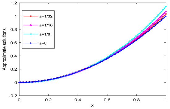
Figure 1. Plot of approximate solutions for different values of $a$ and $R=2$ for Example 1.

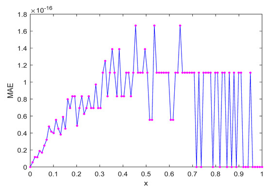
Figure 2. Plot of MAE of Example 1 for R = 2, and $\alpha =\frac{2}{3}$.

Example 2.

Consider the equation with$\alpha =\frac{1}{4}$, n = 1,

$$\begin{gathered} {{\displaystyle \int }}_0^x\left(1-\alpha \right)\left(x-t\right){\mathfrak{D}}^n\left(y\left(t\right)\right)dt+{{\displaystyle \int }}_x^b\left(1-\alpha \right)\left(t-x\right){\mathfrak{D}}^n\left(y\left(t\right)\right)dt-y\left(x\right) – \\ {{\displaystyle \int }}_0^x {\left\{\left(x-t\right)\right\}}^{-1/3}G\left(y\left(t\right)\right)dt=\frac{17}{16}-\frac{3x}{2}-x^2-\frac{x^3}{2}+\frac{3x^4}{8}-\frac{27}{440}{x}^{8/3}\left(11+9x\right), \end{gathered}$$

with initial condition $y\left(0\right)=0$ and exact solution $x^2+x^3$.

We solved this problem by choosing a different number of basis elements R = 2, 3, 4. The corresponding MAE for the different value of$R$ are presented in the Table 1, and the corresponding graph is shown in Figure 3 for R = 3. The approximated solutions of Example $2$are presented in Figure 4 by taking the different value of $\alpha =\frac{1}{4}, \frac{1}{8} , \frac{1}{16}, \frac{1}{32}$ and $\frac{1}{64}$. For $\alpha =\frac{1}{4}$, the numerical solution overlaps the exact solution. Figure 5 shows the relationship between the exact and the approximate solutions of the present example. It is clear that whenever α approaches $\frac{1}{4}$, the numerical solution converges to the exact solution. Table 2 represents the comparison of the MAEs with the method proposed in [29].

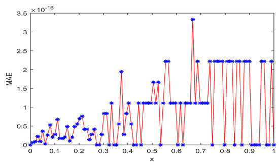
Figure 3. Plot of MAE of Example 2 for $\alpha =\frac{1}{4}$, and R = 3.

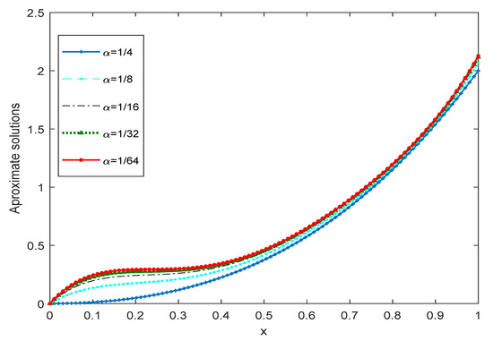
Figure 4. Plot of approximate solutions for different values of α for Example 2.

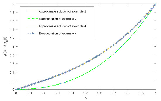
Figure 5. Plot of approximate and exact solutions of Examples 2 and 4.

Table 2. Comparision of MAEs for Example $2$ with the method proposed in [29] for different values of $R.$

R	Present Method	Method [29]
2	$5.55112\times {10}^{-17}$	$2.2891\times {10}^{-2}$
3	$5.55112\times {10}^{-17}$	$2.0455\times {10}^{-16}$

Example 3.

Consider the nonlinear case of the problem Equations (5)–(6) with $\alpha =\frac{1}{2}$, n = 1,

$$\begin{gathered} {{\displaystyle \int }}_0^{\mathrm{x}}(\frac{{\left(x-t\right)}^{-\alpha }}{\Gamma \left(\alpha \right)}{\mathfrak{D}}^n\left(y\left(t\right)\right)dt – q\left(x\right).y\left(x\right)-{{\displaystyle \int }}_0^x {\left\{\left(x\right)\right\}}^{1/2}G\left(y\left(t\right)\right)dt=\frac{2ArcSinh\left(\sqrt{x}\right)}{\sqrt{\pi }\sqrt{1+x}} \\ -\sqrt{x}(-x+\left(1+x\right)ln\left(1+x\right)) – ln\left(1+x\right)\left(2\sqrt{x}+2x^{3/2}-\left(\sqrt{x}+x^{3/2}\right)ln\left(1+x\right)\right), \end{gathered}$$

with $y\left(0\right)=0$, $q\left(x\right)=2\sqrt{x}+2x^{3/2}-\left(\sqrt{x}+x^{3/2}\right)ln\left(1+x\right)$ and the exact solution is $ln\left(1+x\right).$

In this case, the approximation solution is obtained by selecting different values of R = 2, 3, 4, 5, 6, 7, 8, 9, 10 & 11. MAEs corresponding to these cases are calculated, and the corresponding MAE comparison with other polynomials is shown in Table 3. We also plotted the graph of MAE versus R, as shown in Figure 6. It can be observed that as $\mathrm{R}$ increases, MAE tends to zero. A graph between the exact and approximate solutions is presented in Figure 7.

Table 3. Comparision of MAEs for Example 3 with the method given in [29] for different values of R.

R	Present Method	Method [29]
3	$2.3832\times {10}^{-3}$	$2.2891\times {10}^{-3}$
4	$4.3205\times {10}^{-4}$	$2.0455\times {10}^{-5}$
5	$3.7277\times {10}^{-5}$	$4.0699\times {10}^{-5}$
6	$1.8326\times {10}^{-6}$	$4.1765\times {10}^{-6}$

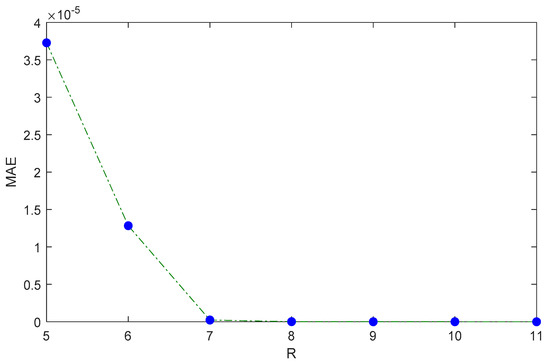
Figure 6. Plot of MAE for different values of R.

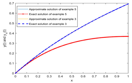
Figure 7. Plot of exact versus approximate solution of Examples 5 and 3.

Example 4.

Consider the problem:

$$\begin{gathered} {{\displaystyle \int }}_0^x\frac{{\left\{d+\left(1-d\right)\left(x-t\right)\right\}}^{-\alpha }}{\Gamma \left(\alpha \right)} {\mathfrak{D}}^n\left(y\left(t\right)\right)dt+{{\displaystyle \int }}_x^b\frac{{\left\{d+\left(1-d\right)\left(t-x\right)\right\}}^{-\alpha }}{\Gamma \left(\alpha \right)}{\mathfrak{D}}^n\left(y\left(t\right)\right)dt-y\left(x\right) \\ -{{\displaystyle \int }}_0^x {\left\{\left(x-t\right)\right\}}^{-\frac{1}{2}}G\left(y\left(t\right)\right)dt -x-x^3-\frac{4}{105}{x}^{ \frac{3}{2}}\left(35+24x^2\right)+\frac{3\left(x^{ \frac{1}{3}}+\frac{27x^{\frac{7}{3}}}{14}\right)}{\Gamma \left( \frac{1}{3}\right)} \\ +\frac{3\left({\left(1-x\right)}^{ \frac{1}{3}}+\frac{3}{14}{\left(1-x\right)}^{ \frac{1}{3}}\left(2+3x+9x^2\right)\right)}{\Gamma \left( \frac{1}{3}\right)}, \end{gathered}$$

with$\alpha =\frac{2}{3}$,$n=1$,$y\left(0\right)=0$. The exact solution of this problem is$x^3+x$.

Here, as in previous cases, we calculate the MAE corresponding to different values of R = 3, 4, 5; the case for R = 4 is shown in Figure 8$.$ We also depict the behavior of the solution by changing the value of $d=\frac{1}{4}, \frac{1}{8} , \frac{1}{16}, \frac{1}{32}$ and $\frac{1}{64}$. Furthermore, as d tends to zero, the approximate solution converges to exact solution, which is shown in Figure 9. In Figure 5, a graph of the exact and the approximate solutions is given.

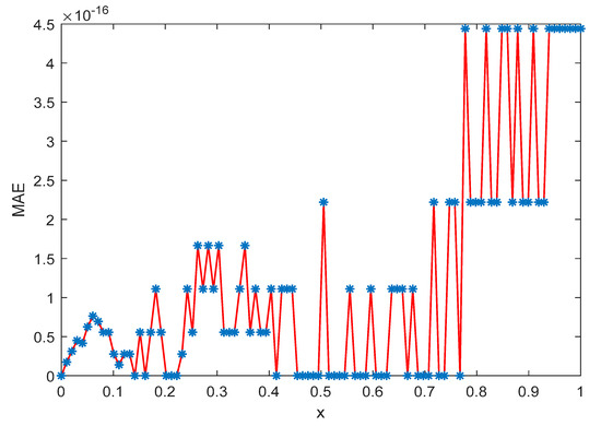
Figure 8. Plot of MAE of Example 4 for $\alpha =\frac{2}{3}$, and R = 4.

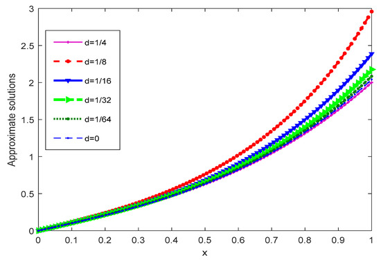
Figure 9. The numerical solutions of Example 4 for different values of d.

Example 5.

Consider,

$$\begin{array}{l}{{\displaystyle \int }}_0^x\left(1-\alpha \right)\left(x-t\right) {\mathfrak{D}}^n\left(y\left(t\right)\right)dt+{{\displaystyle \int }}_x^1\left(1-\alpha \right)\left(t-x\right){\mathfrak{D}}^n\left(y\left(t\right)\right)dt- y\left(x\right) -\\ {{\displaystyle \int }}_0^x {\left\{\left(x-t\right)\right\}}^{-\frac{1}{3}}G\left(y\left(t\right)\right)dt=-e^{-x}-\frac{3\left(-3+x+e^{1-x}\left(1+x\right)\right)}{4e} + \frac{3}{4}\left(1-e^{-x}\left(1+x\right)\right) -\\ \frac{5{\left(-1\right)}^{\frac{1}{3}}{e}^{-x} \Gamma \left(\frac{2}{3}\right)\left(3e^x{\left(-x\right)}^{\frac{5}{3}}-\left(2+3x\right)\left(\Gamma \left(\frac{5}{3}\right)-\Gamma \left(\frac{5}{3} ,-x\right)\right)\right)}{9 \Gamma \left(\frac{8}{3}\right)}.\end{array}$$

This problem has the exact solution$y\left(x\right)=x{e}^{-x}$ with y(0) = 0.

For the given problem, we find the approximate solution by varying the number of elements in the basis and also calculating the corresponding MAEs which are shown in Table 4. The graph of MAE verses $R$ is shown in Figure 10. We notice that the MAE decreases as we increase R, and for R ≥ 11, no change in MAE is observed. In Figure 7, a graph of the exact and the approximate solutions is shown. We also plotted a graph for the MAE for R = 12, as shown in Figure 11.

Table 4. MAEs of Examples 5 and 3 for different values of R.

R	Example 3	Example 5
3	$2.3832\times {10}^{-3}$	$3.35215\times {10}^{-3}$
4	$4.3205\times {10}^{-4}$	$4.78585\times {10}^{-5}$
5	$3.7277\times {10}^{-5}$	$6.86289\times {10}^{-6}$
6	$1.8326\times {10}^{-6}$	$3.02317\times {10}^{-7}$
7	$2.29402\times {10}^{-7}$	$1.23070\times {10}^{-8}$
8	$1.2832\times {10}^{-8}$	$4.513474\times {10}^{-10}$
9	$1.41703\times {10}^{-9}$	$4.58358\times {10}^{-11}$
10	$6.19955\times {10}^{-10}$	$1.906378\times {10}^{-12}$
11	$2.467\times {10}^{-10}$	$1.68061\times {10}^{-13}$
12	$3.2156\times {10}^{-10}$	$1.22863\times {10}^{-13}$

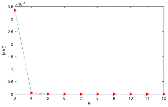
Figure 10. Plot of MAE for different values of R.

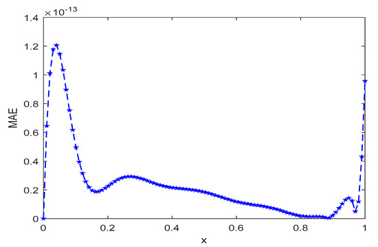
Figure 11. Plot of MAE Example 5 for R = 12.

6. Conclusions

A convergent collocation method is developed in this paper with which to solve GFIDEs in terms of the B-operator. Jacobi poly-fractonomials are used as the basis in the proposed collocation method. The choice of the Jacobi poly-fractonomials helps to increase the accuracy in the approximated solution. The presented method works well on linear and nonlinear types of the GFIDEs and produces accurate solutions.

References

- Srivastava, H.M. Fractional-order derivatives and integrals: Introductory overview and recent developments. Kyungpook Math. J. 2020, 60, 73–116. [Google Scholar]
- Kreyszig, E. Introductory Functional Analysis with Applications; Wiley: New York, NY, USA, 1978. [Google Scholar]
- Podlubny, I. Fractional Differential Equations of Mathematics in Science and Engineering; Academic Press: San Diego, CA, USA, 1999; Volume 198. [Google Scholar]
- Sabatier, J.; Agrawal, O.P.; Machado, J.T. Advances in Fractional Calculus; Springer: Berlin/Heidelberg, Germany, 2007; Volume 4. [Google Scholar]
- Oldham, K.; Spanier, J. The Fractional Calculus Theory and Applications of Differentiation and Integration to Arbitrary Order; Elsevier: Amsterdam, The Netherlands, 1974; Volume 111. [Google Scholar]
- Oldham, K.B.; Spanier, J. The Fractional Calculus, Vol. of Mathematics in Science and Engineering; Academic Press: New York, NY, USA; London, UK, 1974; Volume 111. [Google Scholar]
- Miller, K.S.; Ross, B. An introduction to the Fractional Calculus and Fractional Differential Equations; Wiley: New York, NY, USA, 1993. [Google Scholar]
- Magin, R.L. Fractional calculus in bioengineering, part 2. Critical reviews TM. Biomed Eng. 2004, 32, 195–377. [Google Scholar]
- Goodrich, C.S. Existence of a positive solution to a system of discrete fractional boundary value problems. Appl. Math. Comput. 2011, 217, 4740–4753. [Google Scholar] [CrossRef]
- Oldham, K.B. Fractional differential equations in electrochemistry. Adv. Eng. Softw. 2010, 41, 9–12. [Google Scholar] [CrossRef]
- Engheta, N. On fractional calculus and fractional multipoles in electromagnetism. IEEE Trans. Antennas Propag. 1996, 44, 554–566. [Google Scholar] [CrossRef]
- Saadatmandi, A.; Dehghan, M. A Legendre collocation method for fractional integro-differential equations. J. Vib. Control 2011, 17, 2050–2058. [Google Scholar] [CrossRef]
- Bagley, R.L.; Torvik, P.J. Fractional calculus in the transient analysis of viscoelastically damped structures. AIAA J. 1985, 23, 918–925. [Google Scholar] [CrossRef]
- Tarasov, V.E. Fractional integro-differential equations for electromagnetic waves in dielectric media. Theor. Math. Phys. 2009, 158, 355–359. [Google Scholar] [CrossRef]
- Angell, J.; Olmstead, W.E. Singular perturbation analysis of an integro -differential equation modelling filament stretching. Z. Für Angew. Math. Und Phys. Zamp. 1985, 36, 487–490. [Google Scholar] [CrossRef]
- Khosro, S.; Machado, J.T.; Masti, I. On dual Bernstein polynomials and stochastic fractional integro-differential equations. Math. Methods Appl. Sci. 2020, 43, 9928–9947. [Google Scholar]
- Kilbas, A.A.; Srivastava, H.M.; Trujillo, J.J. Theory and Applications of Fractional Differential Equations; Elsevier: Amsterdam, The Netherlands, 2006; Volume 204. [Google Scholar]
- Yanxin, W.; Zhu, L.; Wang, Z. Fractional-order Euler functions for solving fractional integro-differential equations with weakly singular kernel. Adv. Differ. Equ. 2018, 2018, 254. [Google Scholar]
- Saadatmandi, A.; Dehghan, M. A new operational matrix for solving fractional-order differential equations. Comput. Math. Appl. 2010, 59, 1326–1336. [Google Scholar] [CrossRef]
- Kumar, K.; Pandey, R.K.; Sharma, S. Numerical Schemes for the Generalized Abel’s Integral Equations. Int. J. Appl. Comput. Math. 2018, 4, 68. [Google Scholar] [CrossRef]
- Bonilla, B.; Rivero, M.; Trujillo, J.J. On systems of linear fractional differential equations with constant coefficients. Appl. Math. Comput. 2007, 187, 68–78. [Google Scholar] [CrossRef]
- Momani, S.; Aslam Noor, M. Numerical methods for fourth-order fractional integro-differential equations. Appl. Math. Comput. 2006, 182, 754–760. [Google Scholar] [CrossRef]
- Momani, S.; Qaralleh, R. An efficient method for solving systems of fractional integro-differential equations. Comput. Math. Appl. 2006, 52, 459–470. [Google Scholar] [CrossRef]
- Bhrawy, A.; Zaky, M. Shifted fractional-order Jacobi orthogonal functions: Application to a system of fractional differential equations. Appl. Math. Model. 2016, 40, 832–845. [Google Scholar] [CrossRef]
- Kojabad, E.A.; Rezapour, S. Approximate solutions of a sum-type fractional integro-differential equation by using Chebyshev and Legendre polynomials. Adv. Differ. Equ. 2017, 2017, 1–18. [Google Scholar]
- Rawashdeh, E.A. Numerical solution of fractional integro-differential equations by collocation method. Appl. Math. Comput. 2006, 176, 1–6. [Google Scholar] [CrossRef]
- Syam, M.; Al-Refai, M. Solving fractional diffusion equation via the collocation method based on fractional Legendre functions. J. Comput. Methods Phys. 2014, 2014. [Google Scholar] [CrossRef]
- Eslahchi, M.R.; Dehghan, M.; Parvizi, M. Application of the collocation method for solving nonlinear fractional integro-differential equations. J. Comput. Appl. Math. 2014, 257, 105–128. [Google Scholar] [CrossRef]
- Sharma, S.; Pandey, R.K.; Kumar, K. Collocation method with convergence for generalized fractional integro-differential equations. J. Comput. Appl. Math. 2018, 342, 419–430. [Google Scholar] [CrossRef]
- Odibat, Z.M. Analytic study on linear systems of fractional differential equations. Comput. Math. Appl. 2010, 59, 1171–1183. [Google Scholar] [CrossRef]
- Ma, J.; Liu, J.; Zhou, Z. Convergence analysis of moving finite element methods for space fractional differential equations. J. Comput. Appl. Math. 2014, 255, 661–670. [Google Scholar] [CrossRef]
- Raslan, K.R.; Ali, K.K.; Mohamed, E.M. Spectral Tau method for solving general fractional order differential equations with linear functional argument. J. Egypt. Math. Soc. 2019, 27, 33. [Google Scholar] [CrossRef]
- Zurigat, M.; Momani, S.; Odibat, Z.; Ahmad, A. The homotopy analysis method for handling systems of fractional differential equations. Appl. Math. Model. 2010, 34, 24–35. [Google Scholar] [CrossRef]
- Hassani, H.; Machado, J.T.; Naraghirad, E.; Sadeghi, B. Solving nonlinear systems of fractional-order partial differential equations using an optimization technique based on generalized polynomials. Comput. Appl. Math. 2020, 39, 1–19. [Google Scholar] [CrossRef]
- Agrawal, O.P. Generalized variational problems and Euler–Lagrange equations. Comput. Math. Appl. 2010, 59, 1852–1864. [Google Scholar] [CrossRef]
- Zayernouri, M.; Karniadakis, G.E. Fractional Sturm–Liouville eigen-problems: Theory and numerical approximation. J. Comput. Phys. 2013, 252, 495–517. [Google Scholar] [CrossRef]
Publisher’s Note: MDPI stays neutral with regard to jurisdictional claims in published maps and institutional affiliations. |
© 2021 by the authors. Licensee MDPI, Basel, Switzerland. This article is an open access article distributed under the terms and conditions of the Creative Commons Attribution (CC BY) license (https://creativecommons.org/licenses/by/4.0/).