Unified Polynomial Dynamic Programming Algorithms for P-Center Variants in a 2D Pareto Front ^†

Abstract

With many efficient solutions for a multi-objective optimization problem, this paper aims to cluster the Pareto Front in a given number of clusters K and to detect isolated points. K-center problems and variants are investigated with a unified formulation considering the discrete and continuous versions, partial K-center problems, and their min-sum-K-radii variants. In dimension three (or upper), this induces NP-hard complexities. In the planar case, common optimality property is proven: non-nested optimal solutions exist. This induces a common dynamic programming algorithm running in polynomial time. Specific improvements hold for some variants, such as K-center problems and min-sum K-radii on a line. When applied to N points and allowing to uncover $M<N$ points, K-center and min-sum-K-radii variants are, respectively, solvable in $O\left(K\right(M+1)NlogN)$ and $O\left(K(M+1)N^2\right)$ time. Such complexity of results allows an efficient straightforward implementation. Parallel implementations can also be designed for a practical speed-up. Their application inside multi-objective heuristics is discussed to archive partial Pareto fronts, with a special interest in partial clustering variants.

1. Introduction

This paper is motivated by real-world applications of multi-objective optimization (MOO). Some optimization problems are driven by more than one objective function, with  conflicting optimization directions. For example, one may minimize financial costs, while maximizing the robustness to uncertainties or minimizing the environmental impact  [1,2]. In such cases, higher levels of robustness or sustainability are likely to induce financial over-costs. Pareto dominance, preferring one solution to another if it is better for all the objectives, is a weak dominance rule. With conflicting objectives, several non-dominated points in the objective space can be generated, defining efficient solutions, which are the best compromises. A Pareto front (PF) is the projection in the objective space of the efficient solutions [3]. MOO approaches may generate large sets of efficient solutions using Pareto dominance [3]. Summarizing the shape of a PF may be required for presentation to decision makers. In such a context, clustering problems are useful to support decision making to present a view of a PF in clusters, the density of points in the cluster, or to select the most central cluster points as representative points. Note than similar problems are of interest for population MOO heuristics such as evolutionary algorithms to archive representative points of a partial Pareto fronts, or in selecting diversified efficient solutions to process mutation or cross-over operators [4,5].

With N points in a PF, one wishes to define $K\ll N$ clusters while minimizing the measure of dissimilarity. The K-center problems, both in the discrete and continuous versions, define the cluster costs in this paper, covering the PF with K identical balls while minimizing the radius of the balls used. By definition, the ball centers belong to the PF for the discrete K-center version, whereas the continuous version is similar to geometric covering problems, without any constraint for the localization of centers. Furthermore, sum-radii or sum-diameter are min-sum clustering variants, where the covering balls are not necessarily identical. For each variant, one can also consider partial clustering variants, where a given percentage (or number) of points can be ignored in the covering constraints, which is useful when modelling outliers in the data.

The K-center problems are NP-hard in the general case,  [6] but also for the specific case in ${\mathbb{R}}^2$ using the Euclidean distance [7]. This implies that K-center problems in three-dimensional (3D) PF are also NP-hard, with the planar case being equivalent to an affine 3D PF. We consider the case of two-dimensional (2D) PF in this paper, focusing on the polynomial complexity results. It as an application to bi-objective optimization, the 3D PF and upper dimensions are shown as perspectives after this work. Note that 2D PF are a generalization of one-dimensional (1D) cases, where polynomial complexity results are known [8,9]. A preliminary work proved that K-center clustering variants in a 2D PF are solvable in polynomial time using a Dynamic Programming (DP) algorithm [10]. This paper improves these algorithms for these variants, with an extension to min-sum clustering variants, partial clustering, and Chebyshev and Minkowski distances. The properties of the DP algorithms are discussed for efficient implementation, including parallelization.

This paper is organized as follows. The considered problems are defined formally with unified notations in Section 2. In Section 3, related state-of-the-art elements are discussed. In Section 4 and Section 5, intermediate results and specific complexity results for sub-cases are presented. In Section 6, a unified DP algorithm with a proven polynomial complexity is designed. In Section 7, specific improvements are presented. In Section 8, the implications and applications of the results of Section 5, Section 6 and Section 7 are discussed. In Section 9, our contributions are summarized, with a discussion of future research directions.

2. Problem Statement and Notation

In this paper, integer intervals are denoted as $\left[\right[a,b\left]\right]=[a,b]\cap \mathbb{Z}$. Let $E=\{x_1,\dots ,x_N\}={\left\{x_i\right\}}_{i\in \left[\right[1,N\left]\right]}$ a set of N elements of ${\mathbb{R}}^2$, such that for all $i\ne j$, $x_i\phantom{0}\mathcal{I}\phantom{0}{x}_j$ defining the binary relations $\mathcal{I},\prec$ for all $y=(y^1,y^2),z=(z^1,z^2)\in {\mathbb{R}}^2$ with

$$\begin{array}{ccc}\hfill y\prec z& ⟺& y^1<z^1\phantom{2}\mathrm{and}\phantom{2}{y}^2>z^2\hfill \end{array}$$

(1)

$$\begin{array}{ccc}\hfill y\preccurlyeq z& ⟺& y\prec z\phantom{2}\mathrm{or}\phantom{2}y=z\hfill \end{array}$$

(2)

$$\begin{array}{ccc}\hfill y\phantom{1}\mathcal{I}\phantom{1}z& ⟺& y\prec z\phantom{2}\mathrm{or}\phantom{2}z\prec y\hfill \end{array}$$

(3)

These hypotheses on E define 2D PF considering the minimization of two objectives [3,11]. Such configuration is illustrated by Figure 1. Without loss of generality, transforming objectives to maximize f into $-f$ allows for the consideration of the minimization of two objectives. This assumption impacts the sense of the inequalities of $\mathcal{I},\prec$. A PF can also be seen as a Skyline operator [12]. A 2D PF can be extracted from any subset of ${\mathbb{R}}^2$ using an output-sensitive algorithm [13], or using any MOO approach [3,14].

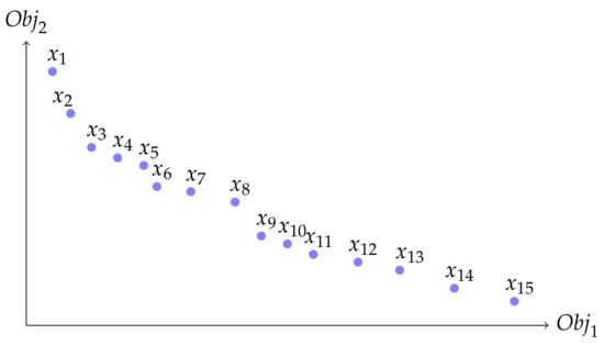
Figure 1. Illustration of a 2D Pareto Front (PF) with 15 points and the indexation implied by Proposition 1.

The results of this paper will be given using the Chebyshev and Minkowski distances, generically denoting $d(y,z)$ the $l_8$ and $l_m$ norm-induced distance, respectively. For a given $m>0$, the Minkowski distance is denoted $d_m$, and given by the formula

$$\forall y=(y^1,y^2),z=(z^1,z^2)\in {\mathbb{R}}^2,d_m(y,z)=\sqrt[m]{{\left|y^1-z^1\right|}^m+{\left|y^2-z^2\right|}^m}$$

(4)

The case $m=2$ corresponds to the Euclidean distance; it is a usual case for our application. The limit with $m\to 8$ defines the Chebyshev distance, denoted $d_8$ and given by the formula

$$\forall y=(y^1,y^2),z=(z^1,z^2)\in {\mathbb{R}}^2,d_8(y,z)=max\left(\left|y^1-z^1\right|,\left|y^2-z^2\right|\right)$$

(5)

Once a distance d is defined, a dissimilarity among a subset of points $E^{\prime }\subset E$ is defined using the radius of the minimal enclosing ball containing $E^{\prime }$. Numerically, this dissimilarity function, denoted as $f_{\mathcal{C}}$, can be written as

$$\forall E^{\prime }\subset E,f_{\mathcal{C}}\left(E^{\prime }\right)=\underset{y\in {\mathbb{R}}^2}{min}\underset{x\in E^{\prime }}{max}d(x,y)$$

(6)

A discrete variant considers enclosing balls with one of the given points as the center. Numerically, this dissimilarity function, denoted $f_{\mathcal{D}}$, can be written as

$$\forall E^{\prime }\subset E,f_{\mathcal{D}}\left(E^{\prime }\right)=\underset{y\in E^{\prime }}{min}\underset{x\in E^{\prime }}{max}d(x,y)$$

(7)

For the sake of having unified notations for common results and proofs, we define $\gamma \in \{0,1\}$ to indicate which version of the dissimilarity function is considered. $\gamma =0$ (respectively,  1) indicates that the continuous (respectively, discrete) version is used, $f_{\gamma }$, thus denoting $f_1=f_{\mathcal{C}}$ (respectively, $f_0=f_{\mathcal{D}}$). Note that $\gamma \in \{0,1\}$ will be related to complexity results which motivated such a notation choice.

For each a subset of points $E^{\prime }\subset E$ and integer $K⩾1$, we define ${\Pi }_K\left(E\right)$, as the set of all the possible partitions of $E^{\prime }$ in K subsets. Continuous and discrete K-center are optimization problems with ${\Pi }_K\left(E\right)$ as a set of feasible solutions, covering E with K identical balls while minimizing the radius of the balls used

$$\underset{\pi \in {\Pi }_K\left(E\right)}{min}\underset{P\in \pi }{max}{f}_{\gamma }\left(P\right)$$

(8)

The continuous and discrete K-center problems in the 2D PF are denoted K-$\gamma$-CP2DPF. Another covering variant, denoted min-sum-K-radii problems, covers the points with non-identical balls, while minimizing the sum of the radius of the balls. We consider the following extension of min-sum-K-radii problems, with $\alpha >0$ being a real number

$$\underset{\pi \in {\Pi }_K\left(E\right)}{min}\sum _{P\in \pi }{f}_{\gamma }{\left(P\right)}^{\alpha }$$

(9)

$\alpha =1$ corresponds to the standard min-sum-K-radii problem. $\alpha =2$ with the standard Euclidean distance is equivalent to the minimization of the area defined by the covering disks. For the sake of unifying notations for results and proofs, we define a generic operator $\oplus \in \{+,max\}$ to denote, respectively, sum-clustering and max-clustering. This defines the generic optimization problems

$$\underset{\pi \in {\Pi }_K\left(E\right)}{min}\underset{P\in \pi }{⨁}{f}_{\gamma }{\left(P\right)}^{\alpha }$$

(10)

Lastly, we consider a partial clustering extension of problems (10), similarly to the partial p-center [15]. The covering with balls mainly concerns the extreme points, which make the results highly dependent on outliers. One may consider that a certain number $M<N$ of the points may be considered outliers, and that M points can be removed in the evaluation. This can be written as

$$\underset{E^{\prime }\subset E:|E\backslash E^{\prime }|⩽M}{min}\underset{\pi \in {\Pi }_K\left(E^{\prime }\right)}{min}\underset{P\in \pi }{⨁}{f}_{\gamma }{\left(P\right)}^{\alpha }$$

(11)

Problem (11) is denoted K-M-⊕-$(\alpha ,\gamma )$-BC2DPF. Sometimes, the partial covering is defined by a maximal percentage of outliers. In this case, if M is much smaller than N, we have $M=\Theta \left(N\right)$, which we have to keep in mind for the complexity results. K-center problems, K-$\gamma$-CP2DPF, are K-M-max-$(\alpha ,\gamma )$-BC2DPF problems for all $\alpha >0$; the value of $\alpha$ does not matter for max-clustering, defining the same optimal solutions as $\alpha =1$. The standard min-sum-k-radii problem, equivalent to the min-sum diameter problem, corresponds to k-0-+-$(1,\gamma )$-BC2DPF problems for discrete and continuous versions, k-M-+-$(1,\gamma )$-BC2DPF problems consider partial covering for min-sum-k-radii problems.

3. Related Works

This section describes works related to our contributions, presenting the state-of-the-art for p-center problems and clustering points in a PF. For more detailed survey on the results for the p-center problems, we refer to [16].

3.1. Solving P-Center Problems and Complexity Results

Generally, the p-center problem consists of locating p facilities among possible locations and assigning n clients, called $c_1,c_2,\dots ,c_n$, to the facilities in order to minimize the maximum distance between a client and the facility to which it is allocated. The continuous p-center problem assumes that any place of location can be chosen, whereas the discrete p-center problem considers a subset o m potential sites, denoted $f_1,f_2,\dots ,f_m$, and distances $d_{i,j}$ for all $i\in \left[\right[1,n\left]\right]$ and $j\in \left[\right[1,m\left]\right]$. Discrete p-center problems can be formulated with bipartite graphs, modeling that si unfeasibile for some assignments. In the discrete p-center problem defined in Section 2, points $f_1,f_2,\dots ,f_m$ are exactly $c_1,c_2,\dots ,c_n$, and the distances are defined using a norm, so that triangle inequality holds for such variants.

P-center problems are NP-hard [6,17]. Furthermore, for all $\alpha <2$, any $\alpha$-approximation for the discrete p-center problem with triangle inequality is NP-hard [18]. Two approximations were provided for the discrete p-center problem running in $O(pnlogn)$ time and in $O\left(np\right)$ time, respecitvely [19,20]. The discrete p-center problem in ${\mathbb{R}}^2$ with a Euclidean distance is also NP-hard [17]. Defining binary variables $x_{i,j}\in \{0,1\}$ and $y_j\in \{0,1\}$ with $x_{i,j}=1$ if and only if the customer i is assigned to the depot j, and $y_j=1$ if and only if location $f_j$ is chosen as a depot, the following Integer Linear Programming (ILP) formulation models the discrete p-center problem [21]

$$\begin{array}{ccccc}{\displaystyle \underset{x,y,z}{min}}\hfill & \hfill z& \hfill & & \left(12\mathrm{a}\right)\hfill \\ s.t:\hfill & \hfill {\displaystyle \sum _{j=1}^n{d}_{i,j}{x}_{i,j}}& ⩽z\hfill & \forall i\in \left[\right[1,n\left]\right]\hfill & \left(12\mathrm{b}\right)\hfill \\ \hfill & \hfill {\displaystyle \sum _{j=1}^m{y}_j}& =p\hfill & \hfill & \left(12\mathrm{c}\right)\hfill \\ \hfill & \hfill {\displaystyle \sum _{j=1}^m{x}_{i,j}}& =1\hfill & \forall i\in \left[\right[1,n\left]\right]\hfill & \left(12\mathrm{d}\right)\hfill \\ \hfill & \hfill x_{i,j}& ⩽y_j\hfill & \forall (i,j)\in \left[\right[1,N\left]\right]\times \left[\right[1,n\left]\right],\hfill & \left(12\mathrm{e}\right)\hfill \\ \hfill & \hfill x_{i,j},y_j& \in \{0,1\}\hfill & \forall i,j\in \left[\right[1,n\left]\right]\times \left[\right[1,m\left]\right],\hfill & \left(12\mathrm{f}\right)\hfill \end{array}$$

Constraints (12b) are implied by a standard linearization of the min–max original objective function. Constraint (12c) fixes the number of open facilities to p. Constraints (12d) assign each client to exactly one facility. Constraints (12e) are necessary to induce that any considered assignment $x_{i,j}=1$ implies that facility j is open with $y_j=1$. Tighter ILP formulations than (12) were proposed, with efficient exact algorithms relying on the IP models [22,23]. Exponential exact algorithms were also designed for the continuous p-center problem [24,25]. An $n^{O\left(\sqrt{p}\right)}$-time algorithm was provided for the continuous Euclidean p-center problem in the plane [26]. An $n^{O\left(p^{1-1/d}\right)}$-time algorithm is available for the continuous p-center problem in ${\mathbb{R}}^d$ under Euclidean and $L_{\infty }$ -metric  [27].

Specific cases of p-center problems are solvable in polynomial time. The continuous 1-center problem is exactly the minimum covering ball problem, which has a linear complexity in ${\mathbb{R}}^2$. Indeed, a “prune and search” algorithm finds the optimum bounding sphere and runs in linear time if the dimension is fixed as a constant [28]. In dimension d, its complexity is in $O\left(\right(d+1\left)\right(d+1)!n)$ time, which is impractical for high-dimensional applications [28]. The discrete 1-center problem is solved in time $O(nlogn)$, using furthest-neighbor Voronoi diagrams [29]. The continuous and planar 2-center problem is solved in randomized expected $O\left(n{log}^{2}n\right)$ time  [30,31]. The discrete and planar 2-center problem is solvable in $O\left(n^{4/3}{log}^{5}n\right)$ time [32].

1D p-center problems, or those with equivalent points that are located in a line, have specific complexity results with polynomial DP algorithms. The discrete 1D k-center problem is solvable in $O\left(n\right)$ time [33]. The continuous and planar k-centers on a line, finding k disks with centers on a given line l, are solvable in polynomial time, in $O\left(n^2{log}^{2}n\right)$ time in the first algorithm by [29], and in $O(nklogn)$ time and $O\left(n\right)$ space in the improved version provided by [34]. An intensively studied extension of the 1D sub-cases is the p-center in a tree structure. The continuous p-center problem is solvable in $O\left(n{log}^{3}n\right)$ time in a tree structure [7]. The discrete p-center problem is solvable in $O(nlogn)$ time in a tree structure [35].

Rectilinear p-center problems, using the Chebyshev distances, were less studied. Such distance is useful for complexity results; however, it has fewer applications than Euclidean or Minkowski norms. For the planar and rectangular 1-center and 2-center problems, $O\left(n\right)$ algorithms are available for the 1-center problem, and such 3-center problems can be solved in $O(nlogn)$ time [36]. In a general dimension d, continuous and discrete versions of rectangular p-center problems are solvable in $O\left(n\right)$ and $O(n{log}^{d-2}nloglogn+nlogn)$ running time, respectively. Specific complexity results for rectangular 2-center problems are also available [37].

3.2. Solving Variants of P-Center Problems and Complexity Results

Variants of p-center problems were studied less intensively than the standard p-center problems. The partial variants were introduced in 1999 by [15], whereas a preliminary work in 1981 considered a partial weighted one-center variant and a DP algorithm to solve it running in $O(n^{2}logn)$ time [38]. The partial discrete p-center can formulated as an ILP starting from the formulation provided by [21] as written in (12). Indeed, considering that $n_0$ points can be uncovered, constraints (12.4) become inequalities ${\sum }_{j=1}^m{x}_{i,j}⩽1$ for all $i,j$ and the maximal number of unassigned points is set to $n_0$, adding one constraint ${\sum }_{j=i}^n{\sum }_{j=1}^m{x}_{i,j}⩾n-n_0$. Similarly, the sum-clustering variants K-M-+-$(\alpha ,\gamma )$-BC2DPF can be written as the following ILP

$$\begin{array}{ccccc}{\displaystyle \underset{z,r⩾0}{min}}\hfill & \hfill {\displaystyle \sum _{n=1}^N{r}_n}& \hfill & & \left(13\mathrm{a}\right)\hfill \\ s.t:\hfill & \hfill {\displaystyle \sum _{n=1}^{N}d{(x_n,x_{n^{\prime }})}^{\alpha }{z}_{n,n^{\prime }}}& ⩽r_{n^{\prime }}\hfill & \forall n^{\prime }\in \left[[1,N]\right]\hfill & \left(13\mathrm{b}\right)\hfill \\ \hfill & \hfill {\displaystyle \sum _{n^{\prime }=1}^N{z}_{n^{\prime },n^{\prime }}}& =K\hfill & \hfill & \left(13\mathrm{c}\right)\hfill \\ \hfill & \hfill {\displaystyle \sum _{n^{\prime }=1}^N{z}_{n,n^{\prime }}}& ⩽1\hfill & \forall n\in \left[\right[1,N\left]\right]\hfill & \left(13\mathrm{d}\right)\hfill \\ \hfill & \hfill {\displaystyle \sum _{n=1}^N\sum _{n^{\prime }=1}^N{z}_{n,n^{\prime }}}& ⩾N-M\hfill & \hfill & \left(13\mathrm{e}\right)\hfill \\ \hfill & \hfill z_{n,n^{\prime }}& ⩽z_{n^{\prime },n^{\prime }}\hfill & \forall (n,n^{\prime })\in {\left[[1,N]\right]}^2,\hfill & \left(13\mathrm{f}\right)\hfill \\ \hfill & \hfill z_{n,n^{\prime }}& \in \{0,1\}\hfill & \forall (n,n^{\prime })\in {\left[[1,N]\right]}^2,\hfill & \left(13\mathrm{g}\right)\hfill \\ \hfill & \hfill r_n& ⩾0\hfill & \forall n\in \left[\right[1,N\left]\right],\hfill & \left(13\mathrm{h}\right)\hfill \end{array}$$

In this ILP formulation, binary variables $z_{n,n^{\prime }}\in \{0,1\}$ are defined such that $z_{n,n^{\prime }}=1$ if and only if the points $x_n$ and $x_{n^{\prime }}$ are assigned in the same cluster, with $x_{n^{\prime }}$ being the discrete center. Continuous variables $r_n⩾0$ denote the powered radius of the ball centered in $x_n$, if $x_n$ is chosen as a center, and  $r_n=0$ otherwise. Constraint (13b) is a standard linearization of the non-linear objective function. $z_{n,n}$ indicates that if point $x_n$ is chosen as the center, then this implies with (13c) that K such variables are nonzero, and with (13f) that a nonzero variable $z_{n,n^{\prime }}$ implies that the corresponding $z_{n^{\prime },n^{\prime }}$ is not null. (13d) and (13e) allow the extension with partial variants, as discussed before.

Min-sum radii or diameter problems were rarely studied. However, such objective functions are useful for meta-heuristics to break some “plateau” effects [39]. Min-sum diameter clustering is NP-hard in the general case and polynomial within a tree structure [40]. The NP-hardness is also proven, even in metrics induced by weighted planar graphs [41]. Approximation algorithms were studied for min-sum diameter clustering. A logarithmic approximation with a constant factor blowup in the number of clusters was provided by [42]. In the planar case with Euclidean distances, a polynomial time approximation scheme was designed [43].

3.3. Clustering/Selecting Points in Pareto Frontiers

Here, we summarize the results related to the selection or the clustering of points in PF, with applications for MOO algorithms. Polynomial complexity resulting in the use of 2D PF structures is an interesting property; clustering problems have a NP-hard complexity in general [17,44,45].

To the best of our knowledge, no specific work focused on PF sub-cases of k-center problems and variants before our preliminary work [10]. A Distance-Based Representative Skyline with similarities to the discrete p-center problem in a 2D PF may not be fully available in the Skyline application, which makes a significant difference [46,47]. The preliminary results proved that K-$\gamma$-CP2DPF is solvable in $O\left(KN{log}^{\gamma }N\right)$ time using $O\left(N\right)$ additional memory space [10]. Partial extensions and min-sum-k-radii variants were not considered for 2D PF. We note that the 2D PF case is an extension of the 1D case, with 1D cases being equivalent to the cases of an affine 2D PF. In the study of complexity results, a tree structure is usually a more studied extension of 1D cases. The discrete k-center problem on a tree structure, and thus the 1D sub-case, is solvable in $O\left(N\right)$ time [33]. 3F PF cases are NP-complete, as already mentioned in the introduction, this being a consequence of the NP-hardness of the general planar case.

Maximization of the quality of discrete representations of Pareto sets was studied with the hypervolume measure in the Hypervolume Subset Selection (HSS) problem [48,49]. The HSS problem is known to be NP-hard in dimension 3 (and greater dimensions) [50]. HSS is solvable with an exact algorithm in $N^{O\left(\sqrt{K}\right)}$ and a polynomial-time approximation scheme for any constant dimension d [50]. The 2D case is solvable in polynomial time with a DP algorithm with a complexity in $O\left(K{N}^2\right)$ time and $O\left(KN\right)$ space [49]. The time complexity of the DP algorithm was improved in $O(KN+NlogN)$ by [51], and in $O\left(K\right(N-K)+NlogN)$ by [52].

The selection of points in a 2D PF, maximizing the diversity, can also be formulated using p-dispersion problems. Max–Min and Max-Sum p-dispersion problems are NP-hard problems [53,54]. Max–Min and Max-Sum p-dispersion problems are still NP-hard problems when distances fulfill the triangle inequality [53,54]. The planar (2D) Max–Min p-dispersion problem is also NP-hard [9]. The one-dimensional (1D) cases of Max–Min and Max-Sum p-dispersion problems are solvable in polynomial time, with a similar DP algorithm running in $O(max\{pN,NlogN\left\}\right)$ time [8,9]. Max–Min p-dispersion was proven to be solvable in polynomial time, with a DP algorithm running in $O(pNlogN)$ time and $O\left(N\right)$ space [55]. Other variants of p-dispersion problems were also proven to be solvable in polynomial time using DP algorithms [55].

Similar results exist for k-means, k-medoid and k-median clustering. K-means is NP-hard for 2D cases, and thus for 3D PF [44]. K-median and K-medoid problems are known to be NP hard in dimension 2, since [17], where the specific case of 2D PF was proven to be solvable in $O\left(N^3\right)$ time with DP algorithms [11,56]. The restriction of k-means to 2D PF would be also solvable in $O\left(N^3\right)$ time with a DP algorithm if a conjecture was proven [57]. We note that an affine 2D PF is a line in ${\mathbb{R}}^2$, where clustering is equivalent to 1D cases. 1D k-means were proven to be solvable in polynomial time with a DP algorithm in $O\left(K{N}^2\right)$ time and $O\left(KN\right)$ space. This complexity was improved for a DP algorithm in $O\left(KN\right)$ time and $O\left(N\right)$ space [58]. This is thus the complexity of K-means in an affine 2D PF.

4. Intermediate Results

4.1. Indexation and Distances in a 2D PF

Lemma 1.

≼ is an order relation, and  ≺ is a transitive relation

$$\forall x,y,z\in {\mathbb{R}}^2,\phantom{3}x\prec y\phantom{1}and\phantom{1}y\prec z⟹x\prec z$$

(14)

Proposition 1 implies an order among the points of E, for a re-indexation in $O(NlogN)$ time

Proposition 1

(Total order). Points $\left(x_i\right)$ can be re-indexed in $O(NlogN)$ time, such that

$$\begin{array}{ccc}\hfill \forall (i_1,i_2)\in {\left[[1;N]\right]}^2,& i_1<i_2⟹& x_{i_1}\prec x_{i_2}\hfill \end{array}$$

(15)

$$\begin{array}{ccc}\hfill \forall (i_1,i_2)\in {\left[[1;N]\right]}^2,& i_1⩽i_2⟹& x_{i_1}\preccurlyeq x_{i_2}\hfill \end{array}$$

(16)

Proof. 

We index E such that the first coordinate is increasing. This sorting procedure runs in $O(NlogN)$ time. Let $(i_1,i_2)\in {\left[[1;N]\right]}^2$, with $i_1<i_2$. We thus have $x_{i_1}^1<x_{i_2}^1$. Having $x_{i_1}\mathcal{I}{x}_{i_2}$ implies that $x_{i_1}^2>x_{i_2}^2$. $x_{i_1}^1<x_{i_2}^1$ and $x_{i_1}^2>x_{i_2}^2$ is by definition $x_{i_1}\prec x_{i_2}$. □

The re-indexation also implies monotonic relations among distances of the 2D PF

Lemma 2.

We suppose that E is re-indexed as in Proposition 1. Letting d be a Minkowski, Euclidean or Chebyshev distance, we obtain the following monotonicity relations

$$\begin{array}{cc}\hfill \forall (i_1,i_2,i_3)\in {\left[[1;N]\right]}^3,& i_1⩽i_2<i_3⟹d(x_{i_1},x_{i_2})<d(x_{i_1},x_{i_3})\end{array}$$

(17)

$$\begin{array}{cc}\hfill \forall (i_1,i_2,i_3)\in {\left[[1;N]\right]}^3,& i_1<i_2⩽i_3⟹d(x_{i_2},x_{i_3})<d(x_{i_1},x_{i_3})\end{array}$$

(18)

Proof. 

We first note that the equality cases are trivial, so we can suppose that $i_1<i_2<i_3$ in the following proof. We prove the propriety (17); the proof of (18) is analogous.

Let $i_1<i_2<i_3$. We note that $x_{i_1}=(x_{i_1}^1,x_{i_1}^2)$, $x_{i_2}=(x_{i_2}^1,x_{i_2}^2)$ and $x_{i_3}=(x_{i_3}^1,x_{i_3}^2)$. Proposition 1 re-indexation ensures $x_{i_1}^1<x_{i_2}^1<x_{i_3}^1$ and $x_{i_1}^2>x_{i_2}^2>x_{i_3}^2$. With $x_{i_3}^1-x_{i_1}^1>x_{i_2}^1-x_{i_1}^1>0$, $|x_{i_1}^1-x_{i_2}^1|<|x_{i_1}^1-x_{i_3}^1|$

With $x_{i_3}^2-x_{i_1}^2<x_{i_2}^2-x_{i_1}^2<0$, $|x_{i_1}^2-x_{i_2}^2|<|x_{i_1}^2-x_{i_3}^2|$

Thus, for any $m>0$, $d_m(x_{i_1},x_{i_2})<|x_{i_1}^1-x_{i_3}^1{|}^m+{|x_{i_1}^2-x_{i_3}^2|}^m=d_m(x_{i_1},x_{i_3})$ and also

$d_8(x_{i_1},x_{i_2})=max\left(\right|x_{i_1}^1-x_{i_2}^1|,|x_{i_1}^2-x_{i_2}^2\left|\right)<max\left(\right|x_{i_1}^1-x_{i_3}^1|,|x_{i_1}^2-x_{i_3}^2\left|\right)=d_8(x_{i_1},x_{i_3})$. Hence, the result is proven for Euclidean, Minkowski and Chebyshev distances. □

4.2. Lemmas Related to Cluster Costs

This section provides the relations needed to compute or compare cluster costs. Firstly, one notes that the computation of cluster costs is easy in a 2D PF in the continuous clustering case.

Lemma 3.

Let $P\subset E$, such that $card\left(P\right)⩾1$. Let i (resp $i^{\prime }$) be the minimal (respective maximal) index of points of P with the indexation of Proposition 1. Then, $f_{\mathcal{C}}\left(P\right)$ can be computed with $f_{\mathcal{C}}\left(P\right)=\frac{1}{2}d(x_i,x_{i^{\prime }})$.

To prove the Lemma 3, we use the Lemmas 4 and 5.

Lemma 4.

Let $P\subset E$, such that $card\left(P\right)⩾1$. Let i (resp $i^{\prime }$) the minimal (resp maximal) index of points of P with the indexation of Proposition 1. We denote with $O=\frac{x_i+x_{i^{\prime }}}{2}$ the midpoint of $x_i,x_{i^{\prime }}$. Then, using a Minkowski or Chebyshev distance d, we have for all $x\in P$: $d\left(x,O\right)⩽d\left(x_i,O\right)=d\left(x_{i^{\prime }},O\right)$.

Proof of Lemma 4: 

We denote with $r=d\left(x_i,O\right)=d\left(x_{i^{\prime }},O\right)=\frac{1}{2}d(x_i,x_{i^{\prime }})$, with the equality being trivial as points $O,x_i,x_{i^{\prime }}$ are on a line and d is a distance. Let $x\in P$. We calculate the distances using a new system of coordinates, translating the original coordinates such that O, is a new origin (which is compatible with the definition of Pareto optimality). $x_i$ and $x_{i^{\prime }}$ have coordinates $(-a,b)$ and $(a,-b)$ in the new coordinate system, with $a,b>0$ and $a^m+b^m=r^m$ if a Minkowski distance is used, otherwise it is $max(a,b)=r$ for the Chebyshev distance. We use $(a^{\prime },b^{\prime })$ to denote the coordinates of x. $x_i\prec x\prec x_{i^{\prime }}$ implies that $-a⩽a^{\prime }⩽a$ and $-b⩽b^{\prime }⩽b$, i.e., $|a^{\prime }|⩽a$ and $|b^{\prime }|⩽b$, which implies $d(x,O)⩽r$, using Minkowski or Chebyshev distances. □

Lemma 5.

Let $P\subset E$ such that $card\left(P\right)⩾1$. Let i (respective $i^{\prime }$) be the minimal (respective maximal) index of points of P with the indexation of Proposition 1. We denote, using $O=\frac{x_i+x_{i^{\prime }}}{2}$, the midpoint of $x_i,x_{i^{\prime }}$. Then, using a Minkowski or Chebyshev distance d, we have for all $y\in {\mathbb{R}}^2$: $d\left(x_i,O\right)=d\left(x_{i^{\prime }},O\right)⩽max(d\left(x_i,y\right),d\left(x_{i^{\prime }},y\right))$.

Proof of Lemma 5: 

As previously noted, let $r=d\left(x_i,O\right)=d\left(x_{i^{\prime }},O\right)=\frac{1}{2}d(x_i,x_{i^{\prime }})$. Let $y\in {\mathbb{R}}^2$. We have to prove that $d\left(x_{i^{\prime }},y\right)⩾r$ or $d\left(x_i,y\right)⩾r$. If we suppose that $d\left(x_i,y\right)<r$, this implies that $y\prec O$. Then, having $y\prec O\prec x_{i^{\prime }}$ implies $d\left(x_{i^{\prime }},y\right)>d\left(x_{i^{\prime }},0\right)=r$ with Lemma 2. □

Proof of Lemma 3: 

We first note that $f_{\mathcal{C}}\left(P\right)={min}_{y\in {\mathbb{R}}^2}{max}_{x\in P}d(x,y)⩽{max}_{x\in P}d\left(x,O\right)$, using the particular point $O=\frac{x_i+x_{i^{\prime }}}{2}$. Using Lemma 4, ${max}_{x\in P}d\left(x,O\right)⩽r$, and thus $f_{\mathcal{C}}\left(P\right)⩽r$ with $r=d\left(x_i,O\right)=d\left(x_{i^{\prime }},O\right)=\frac{1}{2}d(x_i,x_{i^{\prime }})$. Reciprocally, for all $y\in {\mathbb{R}}^2$, $r⩽max(d\left(x_i,y\right),d\left(x_{i^{\prime }},y\right))$ using Lemma 5, and thus $r⩽{max}_{x\in P}d(x,y)$. This implies that $r⩽{min}_{y\in {\mathbb{R}}^2}{max}_{x\in P}d(x,y)=f_{\mathcal{C}}\left(P\right)$. □

Lemma 6.

Let $P\subset E$ such that $card\left(P\right)⩾3$. Let i (respective $i^{\prime }$) the minimal (respective maximal) index of points of P.

$$f_{\mathcal{D}}\left(P\right)=\underset{j\in \left[[i+1,i^{\prime }-1]\right],x_j\in P}{min}max\left(d\left(x_j,x_i\right),d\left(x_j,x_{i^{\prime }}\right)\right)$$

(19)

Proof. 

Let $y\in P-\{x_i,x_{i^{\prime }}\}$. We denote $j\in \left[[i,i^{\prime }]\right]$, such that $y=x_j$. Applying Lemma 2 to $i<j<i^{\prime }$, for all $k\in \left[[i,i^{\prime }]\right],$, we have $d\left(x_j,x_k\right)⩽max\left(d\left(x_j,x_i\right),d\left(x_j,x_i\right)\right)$. Then

$$\begin{array}{ccc}\hfill f_{\mathcal{D}}\left(P\right)& =& \underset{y=x_j\in P}{min}\underset{x\in P}{max}d\left(x,y\right)\hfill \\ \hfill f_{\mathcal{D}}\left(P\right)& =& \underset{j\in \left[[i,i^{\prime }]\right],x_j\in P}{min}max\left(max\left(d\left(x_j,x_i\right),d\left(x_j,x_i\right)\right),\underset{k\in \left[[i,i^{\prime }]\right]}{max}d\left(x_j,x_k\right)\right)\hfill \\ \hfill f_{\mathcal{D}}\left(P\right)& =& \underset{j\in \left[[i,i^{\prime }]\right],x_j\in P}{min}max\left(d\left(x_j,x_i\right),d\left(x_j,x_{i^{\prime }}\right)\right)\hfill \end{array}$$

Lastly, we notice that extreme points are not optimal centers. Indeed, $max\left(d\left(x_i,x_i\right),d\left(x_i,x_{i^{\prime }}\right)\right)=d\left(x_i,x_{i^{\prime }}\right)>max\left(d\left(x_{i+1},x_{i^{\prime }}\right),d\left(x_{i+1},x_i\right)\right)$ with Proposition 2, i.e., i, is not optimal in the last minimization, dominated by $i+1$. Similarly, $i^{\prime }$ is dominated by $i^{\prime }-1$. □

Lemma 7.

Let $\gamma \in \{0,1\}$. Let $P\subset P^{\prime }\subset E$. We have $f_{\gamma }\left(P\right)⩽f_{\gamma }\left(P^{\prime }\right)$.

Proof. 

Using the order of Proposition 1, let i (respectively, $i^{\prime }$) the minimal index of points of P (respectively, $P^{\prime }$) and let j (respectively, $j^{\prime }$) the maximal indexes of points of P (respectively, $P^{\prime }$). $f_{\mathcal{C}}\left(P\right)⩽f_{\mathcal{C}}\left(P^{\prime }\right)$ is trivial using Lemmas 2 and 3. To prove $f_{\mathcal{D}}\left(P\right)⩽f_{\mathcal{D}}\left(P^{\prime }\right)$, we use $i⩽i^{\prime }⩽j^{\prime }⩽j$, and Lemmas 2 and 6

$$\begin{array}{ccc}\hfill f_{\mathcal{D}}\left(P\right)& =& \underset{k\in \left[[i,j]\right],x_k\in P}{min}max\left(d\left(x_k,x_i\right),d\left(x_j,x_k\right)\right)\hfill \\ & ⩽& \underset{k\in \left[[i^{\prime },j^{\prime }]\right],x_k\in P}{min}max\left(d\left(x_k,x_i\right),d\left(x_j,x_k\right)\right)\hfill \\ & ⩽& \underset{k\in \left[[i^{\prime },j^{\prime }]\right],x_k\in P^{\prime }}{min}max\left(d\left(x_k,x_{i^{\prime }}\right),d\left(x_{j^{\prime }},x_k\right)\right)=f_{\mathcal{D}}\left(P^{\prime }\right)\phantom{2}\hfill \end{array}$$

   □

Lemma 8.

Let $\gamma \in \{0,1\}$. Let $P\subset E$, such that $card\left(P\right)⩾1$. Let i (respectively, $i^{\prime }$) the minimal (respectively, maximal) index of points of P. For all $P^{\prime }\subset P$, such that $x_i,x_{i^{\prime }}\in P^{\prime }$, we have $f_{\gamma }\left(P\right)=f_{\gamma }\left(P^{\prime }\right)$

Proof. 

Let $P^{\prime }\subset P$ such that $x_i,x_{i^{\prime }}\in P^{\prime }$. With Lemma 7, we have $f_{\gamma }\left(P^{\prime }\right)⩽f_{\gamma }\left(P\right)$. $f_{\mathcal{C}}\left(P^{\prime }\right)=f_{\mathcal{C}}\left(P\right)$ is trivial using Lemma 3, so that we have to prove $f_{\mathcal{D}}\left(P\right)⩽f_{\mathcal{D}}\left(P^{\prime }\right)$.

${\displaystyle f_{\mathcal{D}}\left(P\right)=\underset{k\in \left[[i,i^{\prime }]\right],x_k\in P}{min}max\left(d\left(x_k,x_i\right),d\left(x_i-x_{i^{\prime }}\right)\right)⩽\underset{k\in \left[[i^{\prime },j^{\prime }]\right],x_k\in P^{\prime }}{min}max\left(d\left(x_k,x_i\right),d\left(x_k,x_{i^{\prime }}\right)\right)=f_{\mathcal{D}}\left(P^{\prime }\right)}$ □

4.3. Optimality of Non-Nested Clustering

In this section, we prove that non-nested clustering property, the extension of interval clustering from 1D to 2D PF, allows the computation of optimal solutions, which will be a key element for a DP algorithm. For  (partial) p-center problems, i.e., K-M-max-$(\alpha ,\gamma )$-BC2DPF, optimal solutions may exist without fulfilling the non-nested property, whereas for K-M-+-$(\alpha ,0)$-BC2DPF problems, the nested property is a necessary condition to obtaining an optimal solution.

Lemma 9.

Let $\gamma \in \{0,1\}$; let $M>0$. There is an optimal solution of 1-M-⊕-$(\alpha ,\gamma )$-BC2DPF on the shape ${\mathcal{C}}_{i,i^{\prime }}={\left\{x_j\right\}}_{j\in \left[[i,i^{\prime }]\right]}=\{x\in E|\exists j\in \left[[i,i^{\prime }]\right],x=x_j\},$ with $|i^{\prime }-i|⩾N-M$.

Proof. 

Let $\pi \in {\Pi }_K\left(E\right)$ represent an optimal solution of 1-M-⊕-$(\alpha ,\gamma )$-BC2DPF, let $OPT$ be the optimal cost, and $\mathcal{C}\subset E$ with $\left|\mathcal{C}\right|⩾N-M$ and $f_{\gamma }\left(\mathcal{C}\right)=OPT$. Let i (respectively, $i^{\prime }$) be the minimal (respectively maximal) index of $\mathcal{C}$ using order of Proposition 1. $\mathcal{C}\subset {\mathcal{C}}_{i,i^{\prime }}$, so Lemma 8 applies and $f_{\gamma }\left({\mathcal{C}}_{i,i^{\prime }}\right)=f_{\gamma }\left(\mathcal{C}\right)=OPT$. $|{\mathcal{C}}_{i,i^{\prime }}|⩾|\mathcal{C}|⩾N-M$, thus ${\mathcal{C}}_{i,i^{\prime }}$ defines an optimal solution of 1-M-⊕-$(\alpha ,\gamma )$-BC2DPF. □

Proposition 2.

Let $E=\left(x_i\right)$ be a 2D PF, re-indexed with Proposition 1. There are optimal solutions of K-M-⊕-$(\alpha ,\gamma )$-BC2DPF using only clusters on the shape ${\mathcal{C}}_{i,i^{\prime }}={\left\{x_j\right\}}_{j\in \left[[i,i^{\prime }]\right]}=\{x\in E|\exists j\in \left[[i,i^{\prime }]\right],x=x_j\}$.

Proof. 

We prove the results by the induction on $K\in {\mathbb{N}}^{*}$. For $K=1$, Lemma 9 gives the initialization.

Let us suppose that $K>1$ and the Induction Hypothesis (IH) that Proposition 2 is true for K-M-⊕-$(\alpha ,\gamma )$-BC2DPF. Let $\pi \in {\Pi }_K\left(E\right)$ be an optimal solution of K-M-⊕-$(\alpha ,\gamma )$-BC2DPF; let $OPT$ be the optimal cost. Let $X\subset E$ be the subset of the non-selected points, $\left|X\right|⩽M$, and ${\mathcal{C}}_1,\dots ,{\mathcal{C}}_K$ be the K subsets defining the costs, so that $X,{\mathcal{C}}_1,\dots ,{\mathcal{C}}_K$ is a partition of E and ${⨁}_{k=1}^K{f}_{\gamma }{\left({\mathcal{C}}_k\right)}^{\alpha }=OPT$. Let $N^{\prime }$ be the maximal index, such that $x_{N^{\prime }}\notin X$, which is, necessarily, $N^{\prime }⩾N-M$. We reindex the clusters ${\mathcal{C}}_k$, such that $x_{N^{\prime }}\in {\mathcal{C}}_K$. Let i be the minimal index such that $x_i\in {\mathcal{C}}_K$.

We consider the subsets ${\mathcal{C}}_K^{\prime }={\left\{x_j\right\}}_{j\in \left[[i,N^{\prime }]\right]}$, $X^{\prime }=X\cap \left[[1,i-1]\right]$ and ${\mathcal{C}}_k^{\prime }={\mathcal{C}}_k\cap {\left\{x_j\right\}}_{j\in \left[\right[1,i-1\left]\right]}$ for all $k\in \left[\right[1,K-1\left]\right]$. It is clear that $X^{\prime },{\mathcal{C}}_1^{\prime },\dots ,{\mathcal{C}}_{K-1}^{\prime }$ is a partition of ${\left\{x_j\right\}}_{j\in \left[\right[1,i-1\left]\right]}$, and $X^{\prime },{\mathcal{C}}_1^{\prime },\dots ,{\mathcal{C}}_K^{\prime }$ is a partition of E. For all $k\in \left[\right[1,K-1\left]\right]$, ${\mathcal{C}}_k^{\prime }\subset {\mathcal{C}}_k$, so that $f_{\gamma }\left({\mathcal{C}}_k^{\prime }\right)⩽f_{\gamma }\left({\mathcal{C}}_k\right)$ (Lemma 7).

$X^{\prime },{\mathcal{C}}_1^{\prime },\dots ,{\mathcal{C}}_K^{\prime }$ is a partition of E, and ${⨁}_{k=1}^K{f}_{\gamma }{\left({\mathcal{C}}_k^{\prime }\right)}^{\alpha }⩽OPT$. ${\mathcal{C}}_1^{\prime },\dots ,{\mathcal{C}}_K^{\prime }$ is an optimal solution of K-$|X^{\prime }|$-⊕-$(\alpha ,\gamma )$-BC2DPF. ${\mathcal{C}}_1^{\prime },\dots ,{\mathcal{C}}_{K-1}^{\prime }$ is an optimal solution of $(K-1)$-$|X^{\prime }|$-⊕-$(\alpha ,\gamma )$-BC2DPF, applied to points $E^{\prime }={\cup }_{k=1}^{K-1}{\mathcal{C}}_1^{\prime }\cup X^{\prime }$. Letting $OP{T}^{\prime }$ be the optimal cost of $(K-1)$-$|X^{\prime }|$-⊕-$(\alpha ,\gamma )$-BC2DPF, we have $OPT=OP{T}^{\prime }\oplus f_{\gamma }{\left({\mathcal{C}}_K^{\prime }\right)}^{\alpha }$. Applying IH for of $(K-1)$-$|X^{\prime }|$-⊕-$(\alpha ,\gamma )$-BC2DPF to points $E^{\prime }$, we have ${\mathcal{C}}_1^{″},\dots ,{\mathcal{C}}_{K-1}^{″}$ an optimal solution of $(K-1)$-$|X^{\prime }|$-⊕-$(\alpha ,\gamma )$-BC2DPF among $E^{\prime }$ on the shape ${\mathcal{C}}_{i,i^{\prime }}={\left\{x_j\right\}}_{j\in 〚i,i^{\prime }〛}=\{x\in E^{\prime }|\exists j\in \left[[i,i^{\prime }]\right],x=x_j\}$. ${⨁}_{k=1}^K{f}_{\gamma }{\left({\mathcal{C}}_k^{″}\right)}^{\alpha }=OP{T}^{\prime }$, and thus ${⨁}_{k=1}^K{f}_{\gamma }{\left({\mathcal{C}}_k^{″}\right)}^{\alpha }\oplus f_{\gamma }{\left({\mathcal{C}}_K^{\prime }\right)}^{\alpha }=OPT$. ${\mathcal{C}}_1^{″},\dots ,{\mathcal{C}}_{K-1}^{″},{\mathcal{C}}_K^{\prime }$ is an optimal solution of K-M-⊕-$(\alpha ,\gamma )$-BC2DPF in E using only clusters ${\mathcal{C}}_{i,i^{\prime }}$. Hence, the result is proven by induction. □

Proposition 3.

There is an optimal solution of K-M-⊕-$(\alpha ,0)$-BC2DPF, removing exactly M points in the partial clustering.

Proof. 

Starting with an optimal solution of K-M-+-$(\alpha ,0)$-BC2DPF, let $OPT$ be the optimal cost, and let $X\subset E$ be the subset of the non-selected points, $\left|X\right|⩽M$, and ${\mathcal{C}}_1,\dots ,{\mathcal{C}}_K$, the K subsets defining the costs, so that $X,{\mathcal{C}}_1,\dots ,{\mathcal{C}}_K$ is a partition of E. Removing random $M-\left|X\right|$ points in ${\mathcal{C}}_1,\dots ,{\mathcal{C}}_K$, we have clusters ${\mathcal{C}}_1^{\prime },\dots ,{\mathcal{C}}_K^{\prime }$ such that, for all $k\in \left[\right[1,K-1\left]\right]$, ${\mathcal{C}}_k^{\prime }\subset {\mathcal{C}}_k$, and thus $f_{\gamma }\left({\mathcal{C}}_k^{\prime }\right)⩽f_{\gamma }\left({\mathcal{C}}_k\right)$ (Lemma 7). This implies ${⨁}_{k=1}^K{f}_{\gamma }{\left({\mathcal{C}}_k^{\prime }\right)}^{\alpha }⩽{⨁}_{k=1}^K{f}_{\gamma }{\left({\mathcal{C}}_k\right)}^{\alpha }=OPT$, and thus the clusters ${\mathcal{C}}_1^{\prime },\dots ,{\mathcal{C}}_K^{\prime }$ and outliers $X^{\prime }=E\backslash {\cup }_k{\mathcal{C}}_k^{\prime }$ define and provide the optimal solution of K-M-⊕-$(\alpha ,0)$-BC2DPF with exactly M outliers. □

Reciprocally, one may investigate if the conditions of optimality in Propositions 2 and 3 are necessary. The conditions are not necessary in general. For instance, with $E=\left\{\right(3,1);(2,2);(1,3\left)\right\}$, $K=M=1$ and the discrete function $F_{\mathcal{D}}$, ie $\gamma =1$, the selection of each pair of points defines an optimal solution, with the same cost as the selection of the three points, which do not fulfill the property of Proposition 3. Having an optimal solution with the two extreme points also does not fulfill the property of Proposition 2. The optimality conditions are necessary in the case of sum-clustering, using the continuous measure of the enclosing disk.

Proposition 4.

Let an optimal solution of K-M-+-$(\alpha ,0)$-BC2DPF be defined with $X\subset E$ as the subset of outliers, with $\left|X\right|⩽M$, and  ${\mathcal{C}}_1,\dots ,{\mathcal{C}}_K$ as the K subsets defining the optimal cost. We therefore have

$\left(i\right)$$\left|{\bigcup }_{k=1}^K{\mathcal{C}}_k\right|=M$, in other words, exactly M points are not selected in π.

$\left(ii\right)$ For each $k\in \left[\right[1,K\left]\right]$, defining $i_k=min\{i\in \left[[1,N]\right]|x_i\in {\mathcal{C}}_k\}$ and $j_k=max\{i\in \left[[1,N]\right]|x_i\in {\mathcal{C}}_k\}$, we have ${\mathcal{C}}_k={\left\{x_i\right\}}_{i\in \left[[i_k,j_k]\right]}$.

Proof. 

Starting with an optimal solution of K-M-+-$(\alpha ,0)$-BC2DPF, let $OPT$ be the optimal cost, and let $X\subset E$ be the subset of the non-selected points, $\left|X\right|⩽M$, and ${\mathcal{C}}_1,\dots ,{\mathcal{C}}_K$ be the K subsets defining the costs, so that $X,{\mathcal{C}}_1,\dots ,{\mathcal{C}}_K$ is a partition of E. We prove $\left(i\right)$ and $\left(ii\right)$ ad absurdum.

If $\left|X\right|<M$, one may remove one extreme point of the cluster ${\mathcal{C}}_1$, defining ${\mathcal{C}}_1^{\prime }$. With Lemmas 2 and 3, we have $f_{\mathcal{C}}\left({\mathcal{C}}_1^{\prime }\right)<f_{\mathcal{C}}\left({\mathcal{C}}_1\right)$, and $f_{\mathcal{C}}{\left({\mathcal{C}}_1^{\prime }\right)}^{\alpha }+{\sum }_{k=1}^K{f}_{\mathcal{C}}{\left({\mathcal{C}}_k\right)}^{\alpha }<f_{\mathcal{C}}{\left({\mathcal{C}}_1\right)}^{\alpha }+{\sum }_{k=1}^K{f}_{\mathcal{C}}{\left({\mathcal{C}}_k\right)}^{\alpha }=OPT$. This is in contraction with the optimality of ${\mathcal{C}}_1,\dots ,{\mathcal{C}}_K$, ${\mathcal{C}}_1^{\prime },{\mathcal{C}}_2\dots ,{\mathcal{C}}_K$, defining a strictly better solution for K-M-+-$(\alpha ,0)$-BC2DPF. $\left(i\right)$ is thus proven ad absurdum.

If $\left(ii\right)$ is not fulfilled by a cluster ${\mathcal{C}}_k$, there is $x_i\notin {\mathcal{C}}_k$ with $i\in \left[[i_k,j_k]\right]$. If $x_i\in X$, we have a better solution than the optimal one with $X^{\prime }=X\cup \left\{x_{i_k}\right\}\backslash \left\{x_i\right\}$ and ${\mathcal{C}}_k^{\prime }={\mathcal{C}}_k\cup \left\{x_i\right\}\backslash \left\{x_{i_k}\right\}$. If $x_i\in {\mathcal{C}}_l$ with $l\ne k$, we have nested clusters ${\mathcal{C}}_l$ and ${\mathcal{C}}_k$. We suppose that $i_k<i_l$ (otherwise, reasoning is symmetrical). We define a better solution than the optimal one with ${\mathcal{C}}_l^{\prime }={\mathcal{C}}_k\cup \left\{x_i\right\}\backslash \left\{x_{i_l}\right\}$ and ${\mathcal{C}}_k^{\prime }={\mathcal{C}}_k\cup \left\{x_{i_l}\right\}\backslash \left\{x_i\right\}$. $\left(ii\right)$ is thus proven ad absurdum. □

4.4. Computation of Cluster Costs

Using Proposition 2, only cluster costs ${\mathcal{C}}_{i,i^{\prime }}$ are computed. This section allows the efficient computation of such cluster costs. Once points are sorted using Proposition 1, cluster costs $f_{\mathcal{C}}\left({\mathcal{C}}_{i,i^{\prime }}\right)$ can be computed in $O\left(1\right)$ using Lemma 3. This makes a time complexity in $O\left(N^2\right)$ to compute all the cluster costs $f_{\mathcal{C}}\left({\mathcal{C}}_{i,i^{\prime }}\right)$ for $1⩽i⩽i^{\prime }⩽N$.

Equation (19) ensures that cluster costs $f_{\mathcal{D}}\left({\mathcal{C}}_{i,i^{\prime }}\right)$ can be computed in $O(i^{\prime }-i)$ for all $i<i^{\prime }$. Actually, Algorithm 1 and Proposition 5 allow for computations in $O(log(i^{\prime }-i))$ once points are sorted following Proposition 1, with a dichotomic and logarithmic search.

Lemma 10.

Letting $(i,i^{\prime })$ with $i<i^{\prime }$. $f_{i,i^{\prime }}:j\in \left[[i,i^{\prime }]\right]⟼max\left(d\left(x_j-x_i\right),d\left(x_j-x_{i^{\prime }}\right)\right)$ decreases before reaching a minimum $f_{i,i^{\prime }}\left(l\right)$, $f_{i,i^{\prime }}(l+1)⩾f_{i,i^{\prime }}\left(l\right)$, and then increases for $j\in \left[[l+1,i^{\prime }]\right]$.

Proof: We define $g_{i,i^{\prime },j},h_{i,i^{\prime },j}$ with $g_{i,i^{\prime }}:j\in \left[[i,i^{\prime }]\right]⟼d\left(x_j-x_i\right)$ and $h_{i,i^{\prime }}:j\in \left[[i,i^{\prime }]\right]⟼d\left(x_j-x_{i^{\prime }}\right)$.

Let $i<i^{\prime }$. Proposition 2, applied to i and any $j,j+1$ with $j⩾i$ and $j<i^{\prime }$, ensures that g is decreasing. Similarly, Proposition 2, applied to $i^{\prime }$ and any $j,j+1$, ensures that h is increasing.

Let $A=\{j\in \left[[i,i^{\prime }]\right]|\forall m\in \left[[i,j]\right]g_{i,i^{\prime }}\left(m\right)<h_{i,i^{\prime }}\left(m\right)\}$.$g_{i,i^{\prime }}\left(i\right)=0$ and $h_{i,i^{\prime }}\left(i\right)=d\left(x_{i^{\prime }}-x_i\right)>0$, so that $i\in A$. A is a non-empty and bounded subset of $\mathbb{N}$, so that A has a maximum. We note that $l=maxA$.$h_{i,i^{\prime }}\left(i^{\prime }\right)=0$ and $g_{i,i^{\prime }}\left(i^{\prime }\right)=d\left(x_{i^{\prime }}-x_i\right)>0$, so that $i^{\prime }\notin A$ and $l<i^{\prime }$.

Let $j\in \left[\right[i,l-1\left]\right]$. $g_{i,i^{\prime }}\left(j\right)<g_{i,i^{\prime }}(j+1)$ and $h_{i,i^{\prime },j}(j+1)<h_{i,i^{\prime }}\left(j\right)$, using the monotony of $g_{i,i^{\prime }}$ and $h_{i,i^{\prime }}$.$f_{i,i^{\prime }}(j+1)=max\left(g_{i,i^{\prime }}(j+1),h_{i,i^{\prime }}(j+1)\right)=h_{i,i}(j+1)$ and $f_{i,i^{\prime }}\left(j\right)=max(g_{i,i^{\prime }}\left(j\right),h_{i,i^{\prime }}\left(j\right))=h_{i,i}\left(j\right)$ as $j,j+1\in A$. Hence, $f_{i,i^{\prime }}(j+1)=h_{i,i^{\prime }}(j+1)<h_{i,i^{\prime }}\left(j\right)=f_{i,i^{\prime }}\left(j\right)$. This proves that $f_{i,i^{\prime }}$ is decreasing in $\left[\right[i,l\left]\right]$.

$l+1\notin A$ and $g_{i,i^{\prime }}(l+1)>h_{i,i^{\prime }}(l+1)$ have to be coherent with the fact that $l=maxA$.

Let $j\in \left[[l+1,i^{\prime }-1]\right]$. $j+1>j⩾l+1$, so $g_{i,i^{\prime }}(j+1)>g_{i,i^{\prime }}\left(j\right)⩾g_{i,i^{\prime }}(l+1)>h_{i,i^{\prime }}(l+1)⩾h_{i,i^{\prime }}\left(j\right)>h_{i,i^{\prime }}(j+1)$ using the monotony of $g_{i,i^{\prime }}$ and $h_{i,i^{\prime }}$.This proves that $f_{i,i^{\prime }}$ is increasing in $\left[[l+1,i^{\prime }]\right]$.

Lastly, the minimum of f can be reached in l or in $l+1$, depending on the sign of $f_{i,i^{\prime }}(l+1)-f_{i,i^{\prime }}\left(l\right)$. If $f_{i,i^{\prime }}(l+1)=f_{i,i^{\prime }}\left(l\right)$, there are two minimums $l,l+1$. Otherwise, there is a unique minimum $l_0\in \{l,l+1\}$, $f_{i,i^{\prime }}$, which decreases before increasing.

Algorithm 1: Computation of $f_{\mathcal{D}}\left({\mathcal{C}}_{i,i^{\prime }}\right)$

input: indexes $i<i^{\prime }$, a distance d

output: the cost $f_{\mathcal{D}}\left({\mathcal{C}}_{i,i^{\prime }}\right)$

define $\underline{i}:=i$, $\underline{v}:=d\left(x_i-x_{i^{\prime }}\right)$, $\overline{i}:=i^{\prime }$, $\overline{v}:=d\left(x_i-x_{i^{\prime }}\right)$,

while$\overline{i}-\underline{i}⩾2$

$i^{″}:=⌊\frac{\overline{i}+\underline{i}}{2}⌋$

if$d\left(x_i-x_{i^{″}}\right)<d\left(x_{i^{\prime }}-x_{i^{″}}\right)$then$\underline{i}:=i^{″}$ and $\underline{v}:=d\left(x_{i^{\prime }}-x_{i^{″}}\right)$

else$\overline{i}:=i^{″}$ and $\overline{v}:=d\left(x_i-x_{i^{″}}\right)$

end while

return$min(\underline{v},\overline{v})$

Proposition 5.

Let $E=\{x_1,\dots ,x_N\}$ be N points of ${\mathbb{R}}^2$, such that for all $i<j$, $x_i\prec x_j$. The computing cost $f_{\mathcal{D}}\left({\mathcal{C}}_{i,i^{\prime }}\right)$ for any cluster ${\mathcal{C}}_{i,i^{\prime }}$ has a complexity in $O(log(i^{\prime }-i))$ time, using $O\left(1\right)$ additional memory space.

Proof. 

Let $i<i^{\prime }$. Let us prove the correctness and complexity of Algorithm 1. Algorithm 1 is a dichotomic and logarithmic search; it iterates $O(log(i^{\prime }-i))$ times, with each iteration running in $O\left(1\right)$ time. The correctness and complexity of Algorithm 1 is a consequence of Lemma 10 and the loop invariant, which exists as a of minimum of $f_{i,i^{\prime }}$, $f_{i,i^{\prime }}\left(j^{*}\right)$ with $\underline{i}⩽j^{*}⩽\overline{i}$, also having $\underline{v}=f_{i,i^{\prime }}\left(\underline{i}\right)$ and $\overline{v}=f_{i,i^{\prime }}\left(\overline{i}\right)$. By construction in Algorithm 1, we have $d\left(x_i-x_{\underline{i}}\right)<d\left(x_{i^{\prime }}-x_{\underline{i}}\right)$, and thus $f_{i,i^{\prime }}\left(\underline{i}\right)=d\left(x_{i^{\prime }}-x_{\underline{i}}\right)$. This implies that $f_{i,i^{\prime }}(\underline{i}-1)=d\left(x_{i^{\prime }}-x_{\underline{i}-1}\right)>f_{i,i^{\prime }}\left(\underline{i}\right)$, and thus $\underline{i}⩽j^{*}$, using Lemma 10. Similarly, we always obtain $d\left(x_i-x_{\underline{i}}\right)⩾d\left(x_{i^{\prime }}-x_{\underline{i}}\right)$, and thus $f_{i,i^{\prime }}\left(\overline{i}\right)=d\left(x_i-x_{\overline{i}}\right)$, $f_{i,i^{\prime }}(\overline{i}+1)=d\left(x_i-x_{\overline{i}+1}\right)>f_{i,i^{\prime }}\left(\overline{i}\right)$, so that $\overline{i}⩾j^{*}$ with Lemma 10. At the convergence of the dichotomic search, $\overline{i}-\underline{i}=1$ and $j^{*}$ is $\underline{i}$ or $\overline{i}$; therefore, the optimal value is $f_{\mathcal{D}}\left({\mathcal{C}}_{i,i^{\prime }}\right)=f_{i,i^{\prime }}\left(j^{*}\right)=min(\underline{v},\overline{v})$.   □

Remark 1.

Algorithm 1 improves the previously proposed binary search algorithm [10]. If it has the same logarithmic complexity, this leads to two times fewer calls of the distance function. Indeed, in the previous version, the dichotomic algorithm is computed at each iteration $f_{i,i^{\prime }}\left(i^{″}\right)$ and $f_{i,i^{\prime }}(i^{″}+1)$ to determine if $i^{″}$ is in the increasing or decreasing phase of $f_{i,i^{\prime }}$. In Algorithm 1, the computations that are provided for each iteration are equivalent to the evaluation of only $f_{i,i^{\prime }}\left(i^{″}\right)$, computing $d\left(x_i-x_{i^{″}}\right)$ and $d\left(x_{i^{\prime }}-x_{i^{″}}\right)$.

Proposition 5 can compute $f_{\mathcal{D}}\left({\mathcal{C}}_{i,i^{\prime }}\right)$ for all $i<i^{\prime }$ in $O(N^{2}logN)$. Now, we prove that the costs $f_{\mathcal{D}}\left({\mathcal{C}}_{i,i^{\prime }}\right)$ of all $i<i^{\prime }$ can be computed in $O\left(N^2\right)$ time instead of $O(N^{2}logN)$ using $O\left(N^2\right)$-independent computations. Two schemes are proposed, computing the lines of the cost matrix in $O\left(N\right)$ time, computing $f_{\mathcal{D}}{\left({\mathcal{C}}_{j,j^{\prime }}\right)}^{\alpha }$ for all $j^{\prime }\in \left[[j;N]\right]$ for a given $j\in \left[\right[1;N\left]\right]$ in Algorithm 2, and computing $f_{\mathcal{D}}{\left({\mathcal{C}}_{j^{\prime },j}\right)}^{\alpha }$ for all $j^{\prime }\in \left[[1;j]\right]$ for a given $j\in \left[\right[1;N\left]\right]$ in Algorithm 3.

Lemma 11.

Let $i,i^{\prime }\in \left[[1,N]\right]$, with $i+1<i^{\prime }$. Let $c\in \left[[i+1,i^{\prime }-1]\right],$ such that $f_{i,i^{\prime }}\left(c\right)=f_{\mathcal{D}}\left({\mathcal{C}}_{i,i^{\prime }}\right)$.

(i) If $i^{\prime }<N$, then there is $c^{\prime }$, such that $c⩽c^{\prime }⩽i^{\prime }$, with  $f_{i,i^{\prime }+1}\left(c^{\prime }\right)={min}_{l\in \left[[i+1,i^{\prime }-1]\right]}{f}_{i,i^{\prime }}\left(l\right)=f_{\mathcal{D}}\left({\mathcal{C}}_{i,i^{\prime }+1}\right)$.

(ii) If $i>1$, then there is $c^{″}$, such that $i⩽c^{\prime }⩽c$, with  $f_{i-1,i^{\prime }}\left(c^{\prime }\right)={min}_{l\in \left[[i+1,i^{\prime }-1]\right]}{f}_{i-1,i^{\prime }}\left(l\right)=f_{\mathcal{D}}\left({\mathcal{C}}_{i-1,i^{\prime }}\right)$.

Proof. 

We prove $\left(i\right)$; we suppose that $i^{\prime }<N$ and we prove that, for all $c^{\prime }<c$$f_{i,i^{\prime }+1}\left(c\right)⩽f_{i,i^{\prime }+1}\left(c^{\prime }\right)$, so that either c is an argmin of the minimization, and the superior minimum to c. $\left(ii\right)$ is similarly proven. Let $c^{\prime }<c$. $f_{i,i^{\prime }}\left(c\right)=f_{\mathcal{D}}\left({\mathcal{C}}_{i,i^{\prime }}\right)$, which implies $f_{i,i^{\prime }}\left(c\right)⩽f_{i,i^{\prime }}\left(c^{\prime }\right)$ and, with Lemma 10, $f_{i,i^{\prime }}$ is decreasing in $\left[[c^{\prime },c]\right]$, i.e., $f_{i,i^{\prime }}\left(c^{″}\right)=d(x_{c^{″}},x_{i^{\prime }})$ for all $c^{″}\in \left[[c^{\prime },c]\right]$ We thus have $d(x_{c^{\prime }},x_{i^{\prime }})⩾d(x_{c^{\prime }},x_i)$, and, with lemma 2, $d(x_{c^{\prime }},x_{i^{\prime }+1})⩾d(x_{c^{\prime }},x_{i^{\prime }})$. Thus, $f_{i,i^{\prime }+1}\left(c^{″}\right)=d(x_{c^{\prime }},x_{i^{\prime }+1}$. With lemma 2, $d(x_{c^{\prime }},x_{i^{\prime }+1}⩾d(x_c,x_{i^{\prime }+1}$. $f_{i,i^{\prime }}\left(c\right)=d(x_c,x_{i^{\prime }})$ implies that $d(x_c,x_{i^{\prime }})⩾d(x_c,x_i)$, and then $d(x_c,x_i)⩽d(x_c,x_{i^{\prime }})⩽d(x_c,x_{i^{\prime }+1})$. Thus $f_{i,i^{\prime }+1}\left(c\right)=d(x_{c^{\prime }},x_{i^{\prime }+1}$, and $f_{i,i^{\prime }}\left(c\right)⩽f_{i,i^{\prime }}\left(c^{\prime }\right)$. □

Proposition 6.

, Let $E=\{x_1,\dots ,x_N\}$ be N points of ${\mathbb{R}}^2$, such that for all $i<j$, $x_i\prec x_j$. Algorithm 2 computes $f_{\mathcal{D}}{\left({\mathcal{C}}_{j,j^{\prime }}\right)}^{\alpha }$ for all $j^{\prime }\in \left[[j;N]\right]$ for a given $j\in \left[\right[1;N\left]\right]$ in $O\left(N\right)$ time using $O\left(N\right)$ memory space.

Proof. 

The validity of Algorithm 2 is based on Lemmas 10 and 11: once a discrete center c is known for a $f_{\mathcal{D}}{\left({\mathcal{C}}_{j,j^{\prime }}\right)}^{\alpha }$, we can find a center $c^{\prime }$ of $f_{\mathcal{D}}{\left({\mathcal{C}}_{j,j^{\prime }+1}\right)}^{\alpha }$ with $c^{\prime }⩾c$, and Lemma 10 gives the stopping criterion to prove a discrete center. Let us prove the time complexity; the space complexity is obviously within $O\left(N\right)$ memory space. In Algorithm 2, each computation $f_{j^{\prime },j}\left(curCtr\right)$ is in $O\left(1\right)$ time; we have to count the number of calls for this function. In each loop in $j^{\prime }$, one computation is used for the initialization; the total number of calls for this initialization is $N-j⩽N$. Then, denoting, with $c_N⩽N$, the center found for ${\mathcal{C}}_{j,N}$, we note that the number of loops is $c_N-j⩽N$. Lastly, there are less that $2N$ computations calls $f_{j^{\prime },j}\left(curCtr\right)$; Algorithm 2 runs in $O\left(N\right)$ time. □

Algorithm 2: Computing $f_{\mathcal{D}}{\left({\mathcal{C}}_{j,j^{\prime }}\right)}^{\alpha }$ for all $j^{\prime }\in \left[[j;N]\right]$ for a given $j\in \left[\right[1;N\left]\right]$

Input:$E=\{x_1,\dots ,x_N\}$ indexed with Proposition 1, $j\in \left[\right[1;N\left]\right]$, $\alpha >0$, N points of ${\mathbb{R}}^2$,

Output: for all $j^{\prime }\in \left[[1;j]\right]$, $v_{j^{\prime }}=f_{\mathcal{D}}^{\alpha }\left({\mathcal{C}}_{j^{\prime },j}\right)$

define vector v with $v_{j^{\prime }}:=0$ for all $j^{\prime }\in \left[[j;N]\right]$

define $curCtr:=j+1$, $curCost:=0$

for$j^{\prime }:=j+1$ to N

$curCost:=f_{j^{\prime },j}\left(curCtr\right)$

while$curCost⩽f_{j^{\prime },j}(curCtr+1)$

$curCtr:=curCtr+1$

$curCost:=f_{j^{\prime },j}\left(curCtr\right)$

end while

$v_{j^{\prime }}:=curCos{t}^{\alpha }$

end for

return vector v

Proposition 7.

Let $E=\{x_1,\dots ,x_N\}$ be N points of ${\mathbb{R}}^2$, such that for all $i<j$, $x_i\prec x_j$. Algorithm 3 computes $f_{\mathcal{D}}{\left({\mathcal{C}}_{j^{\prime },j}\right)}^{\alpha }$ for all $j^{\prime }\in \left[[1;j]\right]$ for a given $j\in \left[\right[1;N\left]\right]$ in $O\left(N\right)$ time, using $O\left(N\right)$ memory space.

Algorithm 3: Computing $f_{\mathcal{D}}{\left({\mathcal{C}}_{j^{\prime },j}\right)}^{\alpha }$ for all $j^{\prime }\in \left[[1;j]\right]$ for a given $j\in \left[\right[1;N\left]\right]$

Input:$E=\{x_1,\dots ,x_N\}$ indexed with Proposition 1, $j\in \left[\right[1;N\left]\right]$, $\alpha >0$, N points of ${\mathbb{R}}^2$,

Output: for all $j^{\prime }\in \left[[1;j]\right]$, $v_{j^{\prime }}=f_{\mathcal{D}}{\left({\mathcal{C}}_{j^{\prime },j}\right)}^{\alpha }$

define vector v with $v_{j^{\prime }}:=0$ for all $j^{\prime }\in \left[[1;j]\right]$

define $curCtr:=j-1$, $curCost:=0$

for$j^{\prime }:=j-1$ to 1 with increment $j^{\prime }:=j^{\prime }-1$

$curCost:=f_{j^{\prime },j}\left(curCtr\right)$

while$curCost⩽f_{j^{\prime },j}(curCtr-1)$

$curCtr:=curCtr-1$

$curCost:=f_{j^{\prime },j}\left(curCtr\right)$

end while

$v_{j^{\prime }}:=curCos{t}^{\alpha }$

end for

return vector v

Proof. 

The proof is analogous with Proposition 6, applied to Algorithm 2. □

5. Particular Sub-Cases

Some particular sub-cases have specific complexity results, which are presented in this section.

5.1. Sub-Cases with $K=1$

We first note that sub-cases $K=1$ show no difference between 1-0-+-$(\alpha ,\gamma )$-BC2DPF and 1-0-max-$(1,\gamma )$-BC2DPF problems, defining the continuous or the discrete version of 1-center problems. Similarly, 1-M-+-$(\alpha ,\gamma )$-BC2DPF and 1-M-max-$(1,\gamma )$-BC2DPF problems define the continuous or the discrete version of partial 1-center problems. 1-center optimization problems have a trivial solution; the unique partition of E in one subset is E. To solve the 1-center problem, it is necessary to compute the radius of the minimum enclosing disk covering all the points of E (centered in one point of E for the discrete version). Once the points are re-indexed with Proposition 1, the cost computation is in $O\left(1\right)$ time for the continuous version using Proposition 3, and in $O(logN)$ time for the discrete version using Proposition 5. The cost of the re-indexation in $O(NlogN)$ forms the overall complexity time with such an approach. One may improve this complexity without re-indexing E.

Proposition 8.

Let $E=\{x_1,\dots ,x_N\}$, a subset of N points of ${\mathbb{R}}^2$, such that for all $i\ne j$, $x_i\phantom{0}\mathcal{I}\phantom{0}{x}_j$. 1-0-⊕-$(\alpha ,\gamma )$-BC2DPF problems are solvable in $O\left(N\right)$ time using $O\left(1\right)$ additional memory space.

Proof. 

Using Lemma 3 or Lemma 6, computations of $f_{\gamma }$ are, at most, in $O\left(N\right)$ once the extreme elements following the order ≺ have been computed. Computation of the extreme points is also seen in $O\left(N\right)$, with one traversal of the elements of E, storing only the current minimal and maximal element with the order relation ≺. Finally, the complexity of one-center problems is in linear time. □

Proposition 9.

Let $M\in {\mathbb{N}}^{*}$, let $E=\{x_1,\dots ,x_N\}$ a subset of N points of ${\mathbb{R}}^2$, such that for all $i\ne j$, $x_i\phantom{0}\mathcal{I}\phantom{0}{x}_j$. The continuous partial 1-center, i.e.,  1-M-⊕-$(\alpha ,0)$-BC2DPF problems, is solvable in $O(Nmin(M,logN\left)\right)$ time. The discrete partial 1-center, i.e.,  1-M-⊕-$(\alpha ,1)$-BC2DPF problems, is solvable in $O(NlogN)$ time.

Proof. 

Using Proposition 2, $one$-center problems are computed equivalently: ${\displaystyle \underset{m\in \left[\right[0;M\left]\right]}{min}{f}_{\gamma }{\left({\mathcal{C}}_{1+m,N-m}\right)}^{\alpha }}$.

For the continuous and the discrete case, re-indexing the whole PF with Proposition 1 runs in $O(NlogN)$ time, leading to M computations in $O\left(1\right)$ or $O(log(N-M\left)\right)$ time, which are dominated by the complexity of re-indexing. The time complexity for both cases are highest in $O(NlogN)$. In the continuous case, i.e., $\gamma =0$, one requires only the M minimal and maximal points with the total order ≺ to compute the cluster costs using. If $M<logN$, one may use one traversal of E, storing the current m minimal and extreme points, which has a complexity in $O\left(MN\right)$. Choosing among the two possible algorithms, the time complexity is in $O(Nmin(M,logN\left)\right)$. □

5.2. Sub-Cases with $K=2$

Specific cases with $K=2$ define two clusters, and one separation as defined in Proposition 2. For these cases, specific complexity results are provided, enumerating all the possible separations.

Proposition 10.

Let N points of ${\mathbb{R}}^2$, $E=\{x_1,\dots ,x_N\}$, such that for all $i\ne j$, $x_i\mathcal{I}{x}_j$. 2-0-⊕-$(\alpha ,\gamma )$-BC2DPF problems are solvable in $O(NlogN)$ time, using $O\left(N^{\gamma }\right)$ additional memory space.

Proof. 

Using Proposition 2, optimal solutions exist, considering two clusters: ${\mathcal{C}}_{1,i}$ and ${\mathcal{C}}_{i+1,N}$. One enumerates the possible separations $i\in \left[\right[1;N\left]\right]$. First, the re-indexation phase runs in $O(NlogN)$ time, which will be the bottleneck for the time complexity. Enumerating the (N-1) values $f_{\gamma }{\left({\mathcal{C}}_{1,i}\right)}^{\alpha }\oplus f_{\gamma }{\left({\mathcal{C}}_{i+1,N}\right)}^{\alpha }$ and storing the minimal value induces (N-1) computations in $O\left(1\right)$ time for the continuous case $\gamma =0$, and uses $O\left(1\right)$ additional memory space: the current best value and the corresponding index. Considering the discrete case, one uses $O\left(N\right)$ additional memory space $f_{\gamma }{\left({\mathcal{C}}_{1,i}\right)}^{\alpha }$, $f_{\gamma }{\left({\mathcal{C}}_{i+1,N}\right)}^{\alpha }$ to maintain the time complexity result. □

One can extend the previous complexity results with the partial covering extension.

Proposition 11.

Let $E=\{x_1,\dots ,x_N\}$ be a subset of N points of ${\mathbb{R}}^2$, such that for all $i\ne j$, $x_i\mathcal{I}{x}_j$. 2-M-⊕-$(\alpha ,\gamma )$-BC2DPF problems are solvable in $O\left(N({(M+1)}^2+logN)\right)$ time and $O\left(N^{\gamma }\right)$ additional memory space, or in $O(N\left({(M+1)}^2{log}^{\gamma }N\right)+logN))$ time and $O\left(1\right)$ additional memory space.

Proof. 

After the re-indexation phase running in $O(logN)$ time), Proposition 2 ensures that there is an optimal solution for 2-M-⊕-$(\alpha ,\gamma )$-BC2DP, removing the $m_1⩾0$ first indexes, the $m_3⩾0$ last indexes, and $m_2⩾0$ points between the two selected clusters, with $m_1+m_2+m_3⩽M$. Using Proposition 3, there is an optimal solution, exactly defining the M outliers, so that we can consider that $m_1+m_2+m_3=M$. Denoting i as the last index of the first cluster, the first selected cluster is ${\mathcal{C}}_{1+m_1,i}$; the second one is ${\mathcal{C}}_{i+m_2+1,N-M+m_1+m_2}$. We have $i⩾m_1+1$ and $i+m_2+1⩽N-M+m_1+m_2$ i.e., $i⩽N-M+m_1$. We denote, with X, the following feasible $i,m_1,m_2$

$$X=\{(i,m_1,m_2)\in \left[[1;N]\right]\times {\left[[0;M]\right]}^2,\phantom{1}0⩽m_1+m_2⩽M\phantom{1}\mathrm{and}\phantom{1}{m}_1+1⩽i⩽N-M+m_1\}$$

Computing an optimal solution for 2-M-⊕-$(\alpha ,\gamma )$-BC2DP brings the following enumeration

$${\displaystyle OPT=\underset{(i,m_1,m_2)\in X}{min}{f}_{\gamma }{\left({\mathcal{C}}_{1+m_1,i}\right)}^{\alpha }+f_{\gamma }{\left({\mathcal{C}}_{i+m_2+1,N-M+m_1+m_2}\right)}^{\alpha }}$$

(20)

In the continuous case (ie $\gamma =0$), we use $O\left({(M+1)}^2\right)$ computations to enumerate the possible $m_1,m_2$, and $O\left(N\right)$ computations to enumerate the possible i once $m_1,m_2$ are defined. With cost computations running in $O\left(1\right)$ time, the computation of (20) by enumeration runs in $O\left(N{(M+1)}^2\right)$ time, after the re-indexation in $O(NlogN)$ time. This induces the time complexity announced for $\gamma =0$. This computation uses $O\left(1\right)$ additional memory space, storing only the best current solution $(i,m_1,m_2)\in X$ and its cost; this is also the announced memory complexity .

In the discrete case (i.e., $\gamma =1$), we use $O({(M+1)}^2)$ computations to enumerate the possible $m_1,m_2$, and $O(N)$ computations to enumerate the possible i once $m_1,m_2$ are fixed. This uses $O(1)$ additional memory space, and the total time complexity is $O(NlogN({(M+1)}^2)$. To decrease the time complexity, one can use two vectors of size N to store a given $m_1,m_2$, for which the cluster costs $f_{\gamma }{\left({\mathcal{C}}_{1+m_1,i}\right)}^{\alpha }$ and $f_{\gamma }{({\mathcal{C}}_{i+m_2+1,N-M+m_1+m_2})}^{\alpha }$ are given by Algorithms 2 and 3, so that the total time complexity remains in $O(N({(M+1)}^2+logN))$ with an $O(N)$ additional memory space. These two variants, using $O\left(1\right)$ or $O\left(N\right)$ additional memory space, induce the time complexity announced in Proposition 11. □

5.3. Continuous Min-Sum K-Radii on A Line

To the best of our knowledge, the 1D continuous min-sum k-radii and the min-sum diameter problems were not previously studied. The specific properties hold, as proven in Lemma 12. This allows a time complexity of $O(NlogN)$.

Lemma 12.

Let $E=\{x_1,\dots ,x_N\}$ be N points in a line of ${\mathbb{R}}^2$, indexed such that for all $i<j$, $x_i\prec x_j$. The min-sum k-radii in a line, K-0-+-$(1,0)$-BC2DPF, is equivalent to selecting the $K-1$ highest values of the distance among consecutive points, with the extremity of such segments defining the extreme points of the disks.

Proof. 

Let a feasible and non-nested solution of K-0-+-$(1,0)$-BC2DPF be defined with clusters ${\mathcal{C}}_{a_1,b_1},{\mathcal{C}}_{a_2,b_2},\dots ,{\mathcal{C}}_{a_K,b_K}$ such that $1=a_1⩽b_1<a_2⩽b_2<\dots <a_K⩽b_K=N$. Using the alignment property, we can obtain

$${\displaystyle d(x_1,x_N)=\sum _{i=1}^{n-1}d(x_i,x_{i+1})=\sum _{k=1}^{K}d(x_{a_k},x_{b_k})+\sum _{k=2}^{K}d(x_{b_{k-1}},x_{a_k})=\sum _{k=1}^K{f}_0\left({\mathcal{C}}_{a_k,b_k}\right)+\sum _{k=2}^{K}d(x_{b_{k-1}},x_{a_k})}$$

Reciprocally, this is equivalent to considering K-0-+-$(1,0)$-BC2DPF or the maximization of the sum of $K-1$ sa a different distance among consecutive points. The latter problem is just computing the $K-1$ highest distances among consecutive points. □

Proposition 12.

Let $E=\{x_1,\dots ,x_N\}$ be a subset of N points of ${\mathbb{R}}^2$ on a line. K-0-+-$(1,0)$-BC2DPF, the continuous min-sum-k-radii, is solvable in $O(NlogN)$ time and $O\left(N\right)$ memory space.

Proof. 

Lemma 12 ensures the validity of Algorithm 4, determining the $K-1$ highest values of the distance among consecutive points. The additional memory space in Algorithm 4 is in O(N), computing the list of consecutive distances. Sorting the distances and the re-indexation both have a time complexity in $O(NlogN)$. □

Algorithm 4: Continuous min-sum K-radii on a line

Input:$K\in {\mathbb{N}}^{*}$, N points of ${\mathbb{R}}^2$ on a line $E=\{x_1,\dots ,x_N\}$

re-index E using Proposition 1

initialize vector v with $v_i:=(i,d\left(x_{i+1}\right)-d\left(x_i\right))$ for $i\in \left[\right[1;N-1\left]\right]$

initialize vector w with $v_j:=0$ for $j\in \left[\right[1;K-1\left]\right]$

sort vector v with $d\left(x_{i+1}\right)-d\left(x_i\right)$ increasing

for the $K-1$ elements of v with the maximal value $d\left(x_{i+1}\right)-d\left(x_i\right)$, store the indexes

i in w

sort w in the increasing order

initialize $\mathcal{P}=\varnothing$, $\underline{i}=\overline{i}=1$, $OPT=0$.

for$j\in \left[\right[1;K-1\left]\right]$ in the increasing order

$\overline{i}:=w_j$

add ${\mathcal{C}}_{\underline{i},\overline{i}}$ in $\mathcal{P}$

$OPT:=OPT+f_{\mathcal{C}}\left({\mathcal{C}}_{\underline{i},\overline{i}}\right)$

$\underline{i}:=\overline{i}+1$

end for

add ${\mathcal{C}}_{\underline{i},N}$ in $\mathcal{P}$

$OPT:=OPT+f_{\mathcal{C}}\left({\mathcal{C}}_{\underline{i},N}\right)$

return$OPT$ the optimal cost and the partition of selected clusters $\mathcal{P}$

6. Unified DP Algorithm and Complexity Results

Proposition 2 allows the design of a common DP algorithm for p-center problems and variants, and to prove polynomial complexities. The key element is to design Bellman equations.

Proposition 13

(Bellman equations). Defining $O_{i,k,m}$ as the optimal cost of k-m-⊕-$(\alpha ,\gamma )$-BC2DPF among points $\left[\right[1,i\left]\right]$ for all $i\in \left[\right[1,N\left]\right]$, $k\in \left[\right[1,K\left]\right]$ and $m\in \left[\right[0,M\left]\right]$, we have the following induction relations

$$\forall i\in \left[[1,N]\right],O_{i,1,0}=f_{\gamma }{\left({\mathcal{C}}_{1,i}\right)}^{\alpha }$$

(21)

$$\forall m\in \left[[1,M]\right],\forall k\in \left[[1,K]\right],\forall i\in \left[[1,m+k]\right],O_{i,k,m}=0$$

(22)

$$\forall m\in \left[[1,M]\right],\forall i\in \left[[m+2,N]\right],O_{i,1,m}=min\left(O_{i-1,1,m-1},f_{\gamma }{\left({\mathcal{C}}_{1+m,i}\right)}^{\alpha }\right)$$

(23)

$$\forall k\in \left[[2,K]\right],\forall i\in \left[[k+1,N]\right],O_{i,k,0}=\underset{j\in \left[\right[k,i\left]\right]}{min}\left(O_{j-1,k-1,0}\oplus f_{\gamma }{\left({\mathcal{C}}_{j,i}\right)}^{\alpha }\right)$$

(24)

$\forall m\in \left[\right[1,M\left]\right],\forall k\in \left[\right[2,K\left]\right],\forall i\in \left[\right[k+m+1,N\left]\right],$

$$\begin{array}{c}\hfill O_{i,k,m}=min\left(O_{i-1,k,m-1},\underset{j\in 〚k+m,i〛}{min}\left(O_{j-1,k-1,m}\oplus f_{\gamma }{\left({\mathcal{C}}_{j,i}\right)}^{\alpha }\right)\right)\end{array}$$

(25)

Proof. (21) is the standard 1-center case. (22) is a trivial case, where it is possible to fill the clusters with singletons, with a null and optimal cost. (23) is a recursion formula among the partial 1-center cases, an optimal solution of 1-m-⊕-$(\alpha ,\gamma )$-BC2DPF among points $\left[\right[1,i\left]\right]$, selecting the point $x_i$, and the optimal solution is cluster ${\mathcal{C}}_{1+m,i}$ with Proposition 3, with a cost $f_{\gamma }{\left({\mathcal{C}}_{1+m,i}\right)}^{\alpha }$ or an optimal solution of 1-$m-1$-⊕-$(\alpha ,\gamma )$-BC2DPF if the point $x_i$ is not selected. (24) is a recursion formula among the k-0-⊕-$(\alpha ,\gamma )$-BC2DPF cases among points $\left[\right[1,i\left]\right]$; when generalizing the ones from [10] for the powered sum-radii cases, the proof is similar. Let $k\in \left[\right[2,K\left]\right]$ and $i\in \left[\right[k+1,N\left]\right]$. Let $j\in \left[\right[k,i\left]\right]$, when selecting an optimal solution of k-0-⊕-$(\alpha ,\gamma )$-BC2DPF among points indexed in $\left[\right[1,j-1\left]\right]$, and adding cluster ${\mathcal{C}}_{j,i}$, a feasible solution is obtained for k-0-⊕-$(\alpha ,\gamma )$-BC2DPF among the points indexed in $\left[\right[1,i\left]\right]$ with a cost $O_{j-1,k-1,0}\oplus f_{\gamma }{\left({\mathcal{C}}_{j,i}\right)}^{\alpha }$. This last cost is lower than the optimal cost, thus $O_{i,k,0}⩽O_{j-1,k-1,0}\oplus f_{\gamma }{\left({\mathcal{C}}_{j,i}\right)}^{\alpha }$. Such inequalities are valid for all $j\in \left[\right[k,i\left]\right]$; this implies

$$O_{i,k,0}⩽\underset{j\in 〚k,i〛}{min}\left(O_{j-1,k-1,0}\oplus f_{\gamma }{\left({\mathcal{C}}_{j,i}\right)}^{\alpha }\right)$$

(26)

Let $j_1<j_2<\dots <j_{k-1}<j_k=i$ indexes, such that ${\mathcal{C}}_{1,j_1},{\mathcal{C}}_{j_1+1,j_2},\dots ,{\mathcal{C}}_{j_{k-1}+1,i}$ defines the optimal solution of k-0-⊕-$(\alpha ,\gamma )$-BC2DPF among the points indexed in $\left[\right[1,i\left]\right]$; its cost is $O_{i,k,0}$. Necessarily, ${\mathcal{C}}_{1,j_1},{\mathcal{C}}_{j_1+1,j_2},\dots ,{\mathcal{C}}_{j_{k-2}+1,j_{k-1}}$ defines the optimal solution of $k-1$-0-⊕-$(\alpha ,\gamma )$-BC2DPF among the points indexed in $\left[[1,j_{k-1}]\right]$. On the contrary, a better solution for $O_{i,k,0}$ would be constructed, adding the cluster ${\mathcal{C}}_{j_{k-1}+1,i}$. We thus have $O_{i,k,0}=O_{j_{k-1},k-1,0}\oplus f_{\gamma }{\left({\mathcal{C}}_{j_{k-1}+1,i}\right)}^{\alpha }$. Combined with (26), this proves $O_{i,k,0}={min}_{j\in 〚k,i〛}\left(O_{j-1,k-1,0}\oplus f_{\gamma }{\left({\mathcal{C}}_{j,i}\right)}^{\alpha }\right)$.

Lastly, we prove (25). Let $m\in \left[\right[1,M\left]\right],k\in \left[\right[2,K\left]\right],i\in \left[\right[k+m+1,N\left]\right]$. $O_{i,k,m}⩽O_{i-1,k,m-1}$; each solution of k-$m-1$-⊕-$(\alpha ,\gamma )$-BC2DPF among the points indexed in $\left[\right[1,i-1\left]\right]$ defines a solution of k-m-⊕-$(\alpha ,\gamma )$-BC2DPF among the points indexed in $\left[\right[1,i\left]\right]$, with the selecting point $x_i$ as an outlier. Let $O_{i,k,m}^{\prime }$, with the cost of k-m-⊕-$(\alpha ,\gamma )$-BC2DPF among the points indexed in $\left[\right[1,i\left]\right]$; necessarily selecting the point i, we obtain $O_{i,k,m}⩽O_{i,k,m}^{\prime }$. $O_{i,k,m}^{\prime }$ is defined by a cluster ${\mathcal{C}}_{j,i}$ and an optimal solution of k-m-⊕-$(\alpha ,\gamma )$-BC2DPF among the points indexed in $\left[\right[1,j-1\left]\right]$, so that $O_{i,k,m}^{\prime }={min}_{j\in \left[\right[k+m,i\left]\right]}\left(O_{j-1,k-1,m}\oplus f_{\gamma }{\left({\mathcal{C}}_{j,i}\right)}^{\alpha }\right)$. We thus have

$$O_{i,k,m}⩽min\left(O_{i-1,k,m-1},\underset{j\in \left[\right[k+m,i\left]\right]}{min}\left(O_{j-1,k-1,m}\oplus f_{\gamma }{\left({\mathcal{C}}_{j,i}\right)}^{\alpha }\right)\right)$$

(27)

Reciprocally, let $1=a_1<b_1<a_2<b_2<\dots <a_k<b_k$ indexes, such that ${\mathcal{C}}_{a_1,b_1},{\mathcal{C}}_{a_2,b_2},\dots ,{\mathcal{C}}_{a_k,b_k}$ defines an optimal solution of k-m-⊕-$(\alpha ,\gamma )$-BC2DPF among the points indexed in $\left[\right[1,i\left]\right]$; its cost is $O_{i,k,m}$. If $b_k=i$, then $O_{i,k,m}=O_{i,k,m}^{\prime }$ and (27) is an equality. If $b_k<i$, then ${\mathcal{C}}_{a_1,b_1},{\mathcal{C}}_{a_2,b_2},\dots ,{\mathcal{C}}_{a_k,b_k}$ defines an optimal solution of k-$m-1$-⊕-$(\alpha ,\gamma )$-BC2DPF among the points indexed in $\left[\right[1,i-1\left]\right]$; its cost is $O_{i,k,m-1}$. We thus have $O_{i,k,m}=O_{i,k,m-1}$, and (27) is an equality. Finally, (25) is proven by disjunction. □

Bellman equations of Proposition 13 can compute the optimal value $O_{i,k,m}$ by induction. A first method is a recursive implementation of the Bellman equations to compute the cost $O_{N,K,M}$ and store the intermediate computations $O_{i,k,m}$ in a memoized implementation. An iterative implementation is provided in Algorithm 5, using a defined order for the computations of elements $O_{i,k,m}$. An advantage of Algorithm 5 is that independent computations are highlighted for a parallel implementation. For both methods computing the optimal cost $O_{N,K,M}$, backtracking operations in the DP matrix with computed costs allow for recovery of the affectation of clusters and outliers in an optimal solution.

In Algorithm 5, note that some useless computations are not processed. When having to compute $O_{N,K,M}$, computations $O_{N,k,m}$ with $k+m<K+M$ are useless. $O_{N-1,K,M}$ will also not be called. Generally, triangular elements $O_{N-n,k,m}$ with $n+k+m<K+M$ are useless. The DP matrix $O_{n,k,m}$ is not fully constructed in Algorithm 5, removing such useless elements.

Algorithm 5: unified DP algorithm for K-M-⊕-$(\alpha ,\gamma )$-BC2DPF

Input: -N points of ${\mathbb{R}}^2$, $E=\{x_1,\dots ,x_N\}$ such that for all $i\ne j$, $x_i\phantom{0}\mathcal{I}\phantom{0}{x}_j$;     - Parameters: $K\in {\mathbb{N}}^{*}$, $M\in \mathbb{N}$, $\oplus \in \{+,max\}$, $\gamma \in \{0,1\}$ and $\alpha >0$;

sort E following the order of Proposition 1

initialize matrix O with $O_{i,k,m}:=0$ for all $m\in \left[\right[0;M\left]\right],k\in \left[\right[1;K-1\left]\right],$

$i\in \left[\right[k;N-K+k\left]\right]$

compute $f_{\gamma }{\left({\mathcal{C}}_{1,i}\right)}^{\alpha }$ for all $i\in \left[\right[1;N-K+1\left]\right]$ and store in $O_{i,1,0}:=f_{\gamma }{\left({\mathcal{C}}_{1,i}\right)}^{\alpha }$

for$i:=2$ to N

compute and store $f_{\gamma }{\left({\mathcal{C}}_{i^{\prime },i}\right)}^{\alpha }$ for all $i^{\prime }\in \left[[1;i]\right]$

compute $O_{i,k,0}:={min}_{j\in \left[\right[k,i\left]\right]}\left(O_{j-1,k-1,0}\oplus f_{\gamma }{\left({\mathcal{C}}_{j,i}\right)}^{\alpha }\right)$ for all $k\in \left[\right[2;min(K,i)\left]\right]$

for$m=1$ to $min(M,i-2)$

compute $O_{i,1,m}:=min\left(O_{i-1,1,m-1},f_{\gamma }{\left({\mathcal{C}}_{1+m,i}\right)}^{\alpha }\right)$

for$k=2$ to $min(K,i-m)$

compute $O_{i,k,m}:=min\left(O_{i-1,k,m-1},{min}_{j\in \left[\right[k+m,i\left]\right]}\left(O_{j-1,k-1,m}\oplus f_{\gamma }{\left({\mathcal{C}}_{j,i}\right)}^{\alpha }\right)\right)$

end for

end for

delete the stored $f_{\gamma }{\left({\mathcal{C}}_{i^{\prime },i}\right)}^{\alpha }$ for all $i^{\prime }\in \left[[1;i]\right]$

end for

initialize $\mathcal{P}=\varnothing$, $\underline{i}=\overline{i}=N$, $m=M$

for$k=K$ to 1 with increment $k\leftarrow k-1$

compute $\overline{i}:=min\{i\in \left[[\underline{i}-m;\underline{i}]\right]|O_{\underline{i},k,m}:=O_{\underline{i}-i,k,m-i+\underline{i}}\}$

$m:=m-\overline{i}+\underline{i}$

compute and store $f_{\alpha }\left({\mathcal{C}}_{i^{\prime },\overline{i}}\right)$ for all $i^{\prime }\in \left[[1;\overline{i}]\right]$

find $\underline{i}\in \left[[1,\overline{i}]\right]$ such that $\underline{i}:=\arg {min}_{j\in \left[\right[k+m,i\left]\right]}\left(O_{j-1,k-1,m}\oplus f_{\gamma }{\left({\mathcal{C}}_{j,\overline{i}}\right)}^{\alpha }\right)$

add ${\mathcal{C}}_{\underline{i},\overline{i}}$ in $\mathcal{P}$

delete the stored $f_{\alpha }\left({\mathcal{C}}_{i^{\prime },\overline{i}}\right)$ for all $i^{\prime }\in \left[[1;\overline{i}]\right]$

end for

return$O_{N,K,M}$ the optimal cost and the selected clusters $\mathcal{P}$

Theorem 1.

Let $E=\{x_1,\dots ,x_N\}$ a subset of N points of ${\mathbb{R}}^2$, such that for all $i\ne j$, $x_i\mathcal{I}{x}_j$. When applied to the 2D PF E for $K⩾2$, the K-M-⊕-$(\alpha ,\gamma )$-BC2DPF problems are solvable to optimality in polynomial time using Algorithm 5, with a complexity in $O\left(K{N}^2(1+M)\right)$ time and $O\left(KN\right(1+M\left)\right)$ space.

Proof. 

The validity of Algorithm 5 is proven by induction; each cell of the DP matrix $O_{i,k,m}$ is computed using only cells that were previously computed to optimality. Once the required cells are computed, a standard backtracking algorithm is applied to compute the clusters. Let us analyze the complexity. Let $K⩾2$. The space complexity is in $O\left(KN\right(1+M\left)\right)$, along with the size of the DP matrix, with the intermediate computations of cluster costs using, at most, O(N) memory space, only remembering such vectors due to the deleting operations. Let us analyze the time complexity. Sorting and indexing the elements of E (Proposition 1) has a time complexity in $O(NlogN)$. Once costs $f_{\gamma }{\left({\mathcal{C}}_{i^{\prime },i}\right)}^{\alpha }$ are computed and stored, each cell of the DP matrix is computed, at most, in $O\left(N\right)$ time using Formulas (21)–(24). This induces a total complexity in $O\left(K{N}^2(1+M)\right)$ time. The cluster costs are computed using N times Algorithm 3 and one time Algorithm 2; this has a time complexity in $O\left(N^2\right)$, which is negligible compared to the $O\left(K{N}^2(1+M)\right)$ time computation of the cells of the DP matrix. The K backtracking operations requires a $O\left(N^2\right)$ time computation of the costs $f_{\alpha }\left({\mathcal{C}}_{i^{\prime },\overline{i}}\right)$ for all $i^{\prime }\in \left[[1;\overline{i}]\right]$ and a given i, M operations in $O\left(1\right)$ time to compute $min\{i\in \left[[\underline{i}-m;\underline{i}]\right]|O_{\underline{i},k,m}=O_{\underline{i}-i,k,m-i+\underline{i}}\}$ and $O\left(N\right)$ operations in $O\left(1\right)$ time to compute $\arg {min}_{j\in \left[\right[k+m,i\left]\right]}\left(O_{j-1,k-1,m}\oplus f_{\gamma }{\left({\mathcal{C}}_{j,\overline{i}}\right)}^{\alpha }\right)$. Finally, the backtracking operations requires $O\left(K{N}^2\right)$ time, which is negligible compared to the previous computation in $O\left(K{N}^2(1+M)\right)$ time. □

7. Specific Improvements

This section investigates how the complexity results of Theorem 2 may be improved, and how to speed up Algorithm 5, from a theoretical and a practical viewpoint.

7.1. Improving Time Complexity for Standard and Partial P-Center Problems

In Algorithm 5, the bottleneck for complexity are the computations ${min}_{j\in \left[\right[k+m,i\left]\right]}\left(O_{j-1,k-1,m}\oplus f_{\gamma }{\left({\mathcal{C}}_{j,i}\right)}^{\alpha }\right)$, for $i\in \left[\right[2,N\left]\right]$, $k\in \left[\right[2,min(K,i)\left]\right]$, $m\in \left[\right[0,i-k\left]\right]$. When $\oplus =max$, it is proven that such a minimization can be processed in $O(logN)$ instead of $O\left(N\right)$ for the naive enumeration, leading to the general complexity results. This can improve the time complexity in the p-center cases.

Lemma 13.

Let $k\in \left[\right[1,K\left]\right]$ and $j\in \left[\right[1,N\left]\right]$. The application $m\in \left[[0,M]\right]⟼O_{j,k,m}$ is decreasing.

Proof. 

Let $m\in \in \left[\right[1,M\left]\right]$. For each $E^{\prime }\subset E$, any feasible solution of k-$(m-1)$-⊕-$(\alpha ,\gamma )$-BC2DPF in $E^{\prime }$ is a feasible solution of k-m-⊕-$(\alpha ,\gamma )$-BC2DPF, with the partial versions defined by problems (11). An optimal solution of k-$m-1$-⊕-$(\alpha ,\gamma )$-BC2DPF is feasible for k-$(m-1)$-⊕-$(\alpha ,\gamma )$-BC2DPF, it implies $O_{j,k,m-1}⩾O_{j,k,m}$. □

Lemma 14.

Let $k\in \left[\right[1,K\left]\right]$ and $m\in \left[\right[0,M\left]\right]$. The application $j\in \left[[1,N]\right]⟼O_{j,k,m}$ is increasing.

Proof. 

We yfirst note that the case $k=1$ is implied by the Lemma 7, so that we can suppose in the following, that $k⩾2$. Let $k\in \left[\right[2,K\left]\right]$, $m\in \left[\right[0,M\left]\right]$ and $j\in \left[\right[2,N\left]\right]$. Let $\pi \in {\Pi }_K\left(E\right)$ be an optimal solution of k-m-⊕-$(\alpha ,\gamma )$-BC2DPF among the points indexed in $\left[\right[1,j\left]\right]$; its cost is $O_{j,k,m}$. Let $X\subset E$, the subset of the non-selected points, $\left|X\right|⩽M$, and ${\mathcal{C}}_1,\dots ,{\mathcal{C}}_k$ with the k subsets defining the costs, so that $X,{\mathcal{C}}_1,\dots ,{\mathcal{C}}_k$ is a partition of E and ${⨁}_{k^{\prime }=1}^k{f}_{\gamma }{\left({\mathcal{C}}_{k^{\prime }}\right)}^{\alpha }=O_{j,k,m}$. If $x_j\in X$, then $O_{j,k,m}=O_{j-1,k,m-1}⩾O_{j-1,k,m}$ using Lemma 13, which is the result. We suppose to end the proof that $x_j\notin X$ and re-index the clusters such that $x_j\in {\mathcal{C}}_k$. We consider the clusters ${\mathcal{C}}_1^{\prime },\dots ,{\mathcal{C}}_k^{\prime }={\mathcal{C}}_1,\dots ,{\mathcal{C}}_{k-1},{\mathcal{C}}_k-x_k$. With X, a partition of ${\left(x_l\right)}_{l\in \left[\right[1,j-1\left]\right]}$ is defined, with, at most, M outliers, so that it defines a feasible solution of the optimization problem, defining $O_{j-1,k,m}$ as a cost $OP{T}^{\prime }⩾O_{j-1,k,m}$. Using Lemma 7, $OP{T}^{\prime }⩽O_{j,k,m}$, so that $O_{j-1,k,m-1}⩾O_{j-1,k,m}$. □

Lemma 15.

Let $i\in \left[\right[2,N\left]\right]$, $k\in \left[\right[2,min(K,i)\left]\right]$, $m\in \left[\right[0,i-k\left]\right]$. Let $g_{i,k,m}:j\in \left[[2,i]\right]⟼max(O_{j-1,k-1,m},f_{\gamma }{\left({\mathcal{C}}_{j,i}\right)}^{\alpha })$. There is $l\in \left[\right[2,i\left]\right]$, such that $g_{i,k}$ is decreasing for $j\in \left[\right[2,l\left]\right]$, and then increases for $j\in \left[\right[l+1,i\left]\right]$. For $j<l$, $g_{i,k}=f_{\gamma }{\left({\mathcal{C}}_{j,i}\right)}^{\alpha }$ and for $j>l$, $g_{i,k}=O_{j-1,k-1,m}$.

Proof. 

Similarly to the proof of Lemma 10, the following applications are monotone:

$j\in \left[[1,i]\right]⟼f_{\gamma }{\left({\mathcal{C}}_{j,i}\right)}^{\alpha }$ decreases with Lemma 7,

$j\in \left[[1,N]\right]⟼O_{j,k,m}$ increases for all k with Lemma 14. □

Proposition 14.

Let $i\in \left[\right[2,N\left]\right],k\in \left[\right[2,K\left]\right],m\in \left[\right[0,M\left]\right]$. Let $\gamma \in \{0,1\}$. Once the values $O_{i^{\prime },k-1,m^{\prime }}$ in the DP matrix of Algorithm 2 are computed, Algorithm 6 computes $O_{i,k,m}={min}_{j\in \left[\right[k+m,i\left]\right]}max\left(O_{j-1,k-1,m},f_{\gamma }{\left({\mathcal{C}}_{j,i}\right)}^{\alpha }\right)$ calling $O(logi)$ cost computations $f_{\gamma }\left({\mathcal{C}}_{j,i}\right)$. This induces a time complexity in $O\left({log}^{1+\gamma }i\right)$ using straightforward computations of the cluster costs with Propositions 3 and 5.

Algorithm 6: Dichotomic computation of ${min}_{j\in \left[\right[k+m,i\left]\right]}max\left(O_{j-1,k-1,m},f_{\gamma }{\left({\mathcal{C}}_{j,i}\right)}^{\alpha }\right)$

input: indexes $i\in \left[\right[2,N\left]\right]$, $k\in \left[\right[2,min(K,i)\left]\right]$, $m\in \left[\right[0,i-k\left]\right]$, $\alpha >0$$\gamma \in \{0,1\}$;

a vector v containing $v_j:=O_{j,k-1,m}$ for all $j\in \left[\right[1,i-1\left]\right]$.

define $\underline{i}:=k+m$, $\underline{v}=f_{\gamma }{\left({\mathcal{C}}_{k+m,i}\right)}^{\alpha }$,

define $\overline{i}:=i$, $\overline{v}:=v_{i-1}$,

while$\overline{i}-\underline{i}⩾2$

$i^{″}:=⌊\frac{\underline{i}+\overline{i}}{2}⌋$

if$f_{\gamma }{\left({\mathcal{C}}_{j,i}\right)}^{\alpha }<v_{i^{″}}$then set $\overline{i}:=i^{″}$ and $\overline{v}:=v_{i^{″}}$

else$\underline{i}:=i^{″}$ and $\underline{v}:=f_{\gamma }{\left({\mathcal{C}}_{j,i}\right)}^{\alpha }$

end while

return$min(\underline{v},\overline{v})$

Proof. 

Algorithm 6 is a dichotomic search based on Lemma 15, similarly to Algorithm 1, derived from Lemma 10. The complexity in Algorithm 6 is $O(logi)$ cost computations $f_{\gamma }\left({\mathcal{C}}_{j,i}\right)$. In the discrete case, such computations run in $O(logi)$ time with Proposition 5, whereas it is $O\left(1\right)$ in the continuous case with Lemma 3. In both cases, the final time complexity is given by $O\left({log}^{1+\gamma }i\right)$. □

Computing ${min}_{j\in \left[\right[k+m,i\left]\right]}max\left(O_{j-1,k-1,m},f_{\gamma }{\left({\mathcal{C}}_{j,i}\right)}^{\alpha }\right)$ in time $O(logi)$ instead of $O\left(i\right)$ in the proof of Theorem 1 for p-center problem and variants, the complexity results are updated for these sub-problems.

Theorem 2.

Let $E=\{x_1,\dots ,x_N\}$ be a subset of N points of ${\mathbb{R}}^2$, such that for all $i\ne j$, $x_i\mathcal{I}{x}_j$. Whe napplied to the 2D PF E for $K⩾2$, the K-M-max-$(\alpha ,\gamma )$-BC2DPF problems are solvable to optimality in polynomial time using Algorithm 4, with a complexity in $O\left(KN\right(1+M)logN)$ time and $O\left(KN\right(1+M\left)\right)$ space.

Proof. 

The validity of Algorithm 5 using Algorithm 6 inside is implied by the validity of Algorithm 6, proven in Proposition 14. Updating the time complexity with Proposition 14, the new time complexity for continuous K-center problems is seen in $O\left(KN\right(1+M)logN)$ time instead of $O\left(K(1+M)N^2\right)$, as previously. For the discrete versions, using Proposition 14 with computations of discrete cluster costs with Proposition 5 induces a time complexity in $O\left(KN(1+M){log}^{2}N\right)$. The complexity is decreased to $O\left(KN\right(1+M)logN)$, where the cluster costs are already computed and stored in Algorithm 5, and thus the computations of Algorithm 6 are seen in $O\left(1\right)$. tThisinduces the same complexity for discrete and continuous K-center variants. □

Remark 2.

For the standard discrete p-center, Theorem 2 improves the time complexity given in the preliminary paper [10], from $O\left(pN{log}^{2}N\right)$ to $O(pNlogN)$. Another improvement was given by Algorithm 1; the former computation of cluster costs has the same asymptotic complexity but requires two times more computations. tTis proportional factor is non negligible in practice.

7.2. Improving Space Complexity for Standard P-Center Problems

For standard p-center problems, Algorithm 5 has a complexity in memory space in $O\left(KN\right)$, the size of the DP matrix. This section proves it is possible to reduce the space complexity into an $O\left(N\right)$ memory space.

One can compute the DP matrix for k-centers “line-by-line”, with k increasing. This does not change the validity of the algorithm, with each computation using values that were previously computed to the optimal values. Two main differences occur compared to Algorithm 5. On one hand, the $k+1$-center values use only k-center computations, and the computations with $k^{\prime }<k$ can be deleted once all the required k-center values are computed when having to compute only the K-center values, especially the optimal cost. On the other hand, the  computations of cluster costs are not factorized, as in Algorithm 5; this does not make any difference in the continuous version, where Lemma 3 can to recompute cluster costs in $O\left(1\right)$ time when needed, whereas recomputing each cost induces the computations running in $O(logN)$ for the discrete version with Algorithm 1.

The search order of operations slightly degrades the time complexity for the discrete variant, without inducing a change in the continuous variant. This allows only for computations of the optimal value; another difficulty is that the backtracking operations, as written in Algorithm 5, require storage of the whole stored values of the whole matrix. The issue is obtaining alternative backtracking algorithms that allow the computation of an optimal solution of the standard p-center problems using only the optimal value provided by the DP iterations, and with a complexity of, at most, $O\left(KN{log}^{\gamma }N\right)$ time and $O\left(N\right)$ memory space. Algorithms 7 and 8 have such properties.

Algorithm 7: Backtracking algorithm using $O\left(N\right)$ memory space

input: - $\gamma \in \{0,1\}$ to specify the clustering measure;

- N points of a 2D PF, $E=\{z_1,\dots ,z_N\}$, sorted such that for all $i<j$, $z_i\prec z_j$;

- $K\in \mathbb{N}$ the number of clusters;

- $OPT$, the optimal cost of K-$\gamma$-CP2DPF;

output: $\mathcal{P}$ an optimal partition of K-$\gamma$-CP2DPF.

initialize $maxId:=N$, $minId:=N$, $\mathcal{P}=⌀$, a set of sub-intervals of $\left[\right[1;N\left]\right]$.

for$k:=K$ to 2 with increment $k\leftarrow k-1$

set $minId:=maxId$

while$f_{\gamma }\left({\mathcal{C}}_{minId-1,maxId}\right))⩽OPT$do$minId:=minId-1$end while

add $\left[\right[minId,maxId\left]\right]$ in $\mathcal{P}$

$maxId:=minId-1$

end for

add $\left[\right[1,maxId\left]\right]$ in $\mathcal{P}$

return$\mathcal{P}$

Algorithm 8: Backtracking algorithm using $O\left(N\right)$ memory space

input: - $\gamma \in \{0,1\}$ to specify the clustering measure;

- N points of a 2D PF, $E=\{z_1,\dots ,z_N\}$, sorted such that for all $i<j$, $z_i\prec z_j$;

- $K\in \mathbb{N}$ the number of clusters;

- $OPT$, the optimal cost of K-$\gamma$-CP2DPF;

output: $\mathcal{P}$ an optimal partition of K-$\gamma$-CP2DPF.

initialize $minId:=1$, $maxId:=1$, $\mathcal{P}:=⌀$, a set of sub-intervals of $\left[\right[1;N\left]\right]$.

for$k:=2$ to K with increment $k\leftarrow k+1$

set $maxId:=minId$

while$f_{\gamma }\left({\mathcal{C}}_{minId,maxId+1}\right))⩽OPT$do$maxId:=maxId+1$end while

add $\left[\right[minId,maxId\left]\right]$ in $\mathcal{P}$

set $minId:=maxId+1$

end for

add $\left[\right[minId,N\left]\right]$ in $\mathcal{P}$

return$\mathcal{P}$

Lemma 16.

Let $K\in \mathbb{N},K⩾2$. Let $E=\{z_1,\dots ,z_N\}$, sorted such that for all $i<j$, $z_i\phantom{0}\prec \phantom{0}{z}_j$. For the discrete and continuous K-center problems, the indexes given by Algorithm 7 are lower bounds of the indexes of any optimal solution. Denoting $\left[[1,i_1]\right],\left[[i_1+1,i_2]\right],\dots ,\left[[i_{K-1}+1,N]\right]$, the indexes given by Algorithm 7, and $\left[[1,i_1^{\prime }]\right],\left[[i_1^{\prime }+1,i_2^{\prime }]\right],\dots ,\left[[i_{K-1}^{\prime }+1,N]\right]$, the indexes of an optimal solution, we have, for all $k\in \left[[1,K-1]\right],i_k⩽i_k^{\prime }$

Proof. 

This lemma is proven a decreasing induction on k, starting from $k=K-1$. The case $k=K-1$ is furnished by the first step of Algorithm 4, and $j\in \left[[1,N]\right]⟼f_{\gamma }\left({\mathcal{C}}_{j,N}\right)$ decreaswa with Lemma 7. WIth a given k, $i_k^{\prime }⩽i_k$, $i_{k-1}⩽i_{k-1}^{\prime }$ is implied by Lemma 2 and $d(z_{i_k},z_{i_{k-1}-1})>OPT$. □

Algorithm 8 is similar to Algorithm 7, with iterations increasing the indexes of the points of E. The validity is similarly proven, and this provides the upper bounds for the indexes of any optimal solution of K-center problems.

Lemma 17.

Let $K\in \mathbb{N},K⩾2$. Let $E=\{z_1,\dots ,z_N\}$, sorted such that for all $i<j$, $z_i\phantom{0}\prec \phantom{0}{z}_j$. For K-center problems, the indexes given by Algorithm 8 are upper bounds of the indexes of any optimal solution. Denoting $\left[[1,i_1]\right],\left[[i_1+1,i_2]\right],\dots ,\left[[i_{K-1}+1,N]\right]$, the indexes given by Algorithm 8, and $\left[[1,i_1^{\prime }]\right],\left[[i_1^{\prime }+1,i_2^{\prime }]\right],\dots ,\left[[i_{K-1}^{\prime }+1,N]\right]$, the indexes of an optimal solution, we have, for all $k\in \left[[1,K-1]\right],i_k⩾i_k^{\prime }$.

Proposition 15.

Once the optimal cost of p-center problems are computed, Algorithms 7 and 8 compute an optimal partition in $O(NlogN)$ time using $O\left(1\right)$ additional memory space.

Proof. 

We consider the proof for Algorithm 7, which is symmetrical for Algorithm 8. Let $OPT$ be the optimal cost of K-center clustering with f. Let $\left[[1,i_1]\right],\left[[i_1+1,i_2]\right],\dots ,\left[[i_{K-1}+1,N]\right]$ be the indexes given by Algorithm 7. Through this construction, all the clusters $\mathcal{C}$ defined by the indexes $\left[[i_k+1,i_{k+1}]\right]$ for all $k>1$ verify $f_{\gamma }\left(\mathcal{C}\right)⩽OPT$. Let ${\mathcal{C}}_1$ be the cluster defined by $\left[[1,i_1]\right]$; we have to prove that $f_{\gamma }\left({\mathcal{C}}_1\right)⩽OPT$ to conclude the optimality of the clustering defined by Algorithm 4. For an optimal solution, let $\left[[1,i_1^{\prime }]\right],\left[[i_1^{\prime }+1,i_2^{\prime }]\right],\dots ,\left[[i_{K-1}^{\prime }+1,N]\right]$ be the indexes defining this solution. Lemma 16 ensures that $i_1⩽i_1^{\prime }$, and thus Lemma 7 assures $f_{\gamma }\left({\mathcal{C}}_{1,i_1}\right)⩽f_{\gamma }\left({\mathcal{C}}_{1,i_1^{\prime }}\right)⩽OPT$. Analyzing the complexity, Algorithm 7 calls for a maximum of $(K+N)⩽2N$ times the clustering cost function, without  requiring stored elements; the complexity is in $O\left(N{log}^{\gamma }N\right)$ time. □

Remark 3.

Finding the biggest cluster with an extremity given and a bounded cost can be acheived by a dichotomic search. Rhis would induce a complexity in $O\left(K{log}^{1+\gamma }N\right)$. To avoid the separate case $K=O\left(N\right)$ and $\gamma =1$, Algorithms 7 and 8 provide a common algorithm running in $O(NlogN)$ time, which is enough for the following complexity results.

The previous improvements, written in Algorithm 9, allow for new complexity results with a $O\left(N\right)$ memory space for K-centrer problems.

Algorithm 9: p-center clustering in a 2DPF with a O(N) memory space

Input:

- N points of ${\mathbb{R}}^2$, $E=\{x_1,\dots ,x_N\}$ such that for all $i\ne j$, $x_i\phantom{0}\mathcal{I}\phantom{0}{x}_j$;

- $\gamma \in \{0,1\}$ to specify the clustering measure;

- $K\in \mathbb{N}$ the number of clusters.

initialize matrix O with $O_{i,k}:=0$ for all $i\in \left[\right[1;N\left]\right],k\in \left[\right[1;K-1\left]\right]$

sort E following the order of Proposition 1

compute and store $O_{i,1}:=f_{\gamma }\left({\mathcal{C}}_{1,i}\right)$ for all $i\in \left[\right[1;N\left]\right]$ (with Algorithm 2 if $\gamma =1$)

for$k=2$ to $K-1$

for$i=k+1$ to $N-K+k$

compute and store $O_{i,k}:={min}_{j\in \left[\right[2,i\left]\right]}max(O_{j-1,k-1},f_{\gamma }\left({\mathcal{C}}_{j,i}\right))$ (Algorithm 6)

end for

delete the stored $O_{i,k-1}$ for all i

end for

$OPT:={min}_{j\in \left[\right[2,N\left]\right]}max(O_{j-1,K-1},f_{\gamma }\left({\mathcal{C}}_{j,N}\right))$ with Algorithm 6

return$OPT$ the optimal cost and a partition $\mathcal{P}$ given by backtracking Algorithm 7 or 8

Theorem 3.

Let $E=\{x_1,\dots ,x_N\}$ a subset of N points of ${\mathbb{R}}^2$, such that for all $i\ne j$, $x_i\mathcal{I}{x}_j$. When applied to the 2D PF E for $K⩾2$, the standard continuous and discrete K-center problems, i.e., K-0-max-$(\alpha ,\gamma )$-BC2DPF, are solvable with a complexity in $O\left(KN{log}^{1+\gamma }N\right)$ time and $O\left(N\right)$ space.

Remark 4.

The continuous case improves the complexity obtained after Theorem 2, with the same time complexity and an improvement in the space complexity. For the discrete variant, improving the space complexity in $O\left(N\right)$ instead of $O\left(N\right)$ induces a very slight degradation of the time complexity, from $O(KNlogN)$ to $O\left(KN{log}^{2}N\right)$. Depending on the value of K, it may be preferable, with stronger constraints in memory space, to have this second version.

7.3. Improving Space Complexity for Partial P-Center Problems?

This section tries to generalize the previous results for the partial K-center problems, i.e., K-M-max-$(\alpha ,\gamma )$-BC2DPF with $M>0$. The key element is to obtain a backtracking algorithm that does not use the DP matrix. Algorithm 10 extends Algorithm 7 by considering all the possible cardinals of outliers between clusters k and $k+1$ for $k\in \left[\right[0,K-1\left]\right]$ and the outliers after the last cluster. A feasible solution of the optimal cost should be feasible by iterating Algorithm 7 for at least one of these sub-cases.

Algorithm 10: Backtracking algorithm for K-M-max-$(\alpha ,\gamma )$-BC2DPF with $M>0$

input: - a K-M-max-$(\alpha ,\gamma )$-BC2DPF problem

- N points of a 2D PF, $E=\{z_1,\dots ,z_N\}$, sorted such that for all $i<j$, $z_i\prec z_j$;

- $OPT$, the optimal cost of K-M-max-$(\alpha ,\gamma )$-BC2DPF problem;

output: $\mathcal{P}$ an optimal partition of K-M-max-$(\alpha ,\gamma )$-BC2DPF problem.

for each vector x of $K+1$ elements such that ${\sum }_{k=0}^{K}x\left[k\right]=M$

initialize $maxId-x\left[K\right]:=N$, $minId:=N-x\left[K\right]$, $\mathcal{P}:=⌀$, a set of sub-intervals

of $\left[\right[1;N\left]\right]$.

for$k=K$ to 2 with increment $k\leftarrow k-1$

set $minId:=maxId$

while$f_{\gamma }\left({\mathcal{C}}_{minId-1,maxId}\right){)}^{\alpha }⩽OPT$do$minId:=minId-1$end while

add $\left[\right[minId,maxId\left]\right]$ in $\mathcal{P}$

set $maxId:=minId-1-x[K-1]$

end for

if$f_{\gamma }\left({\mathcal{C}}_{1+x\left[0\right],maxId}\right){)}^{\alpha }⩽OPT$then add $\left[\right[1+x\left[0\right],maxId\left]\right]$ in $\mathcal{P}$ and return $\mathcal{P}$

end for

return error “OPT is not a feasible cost for K-M-max-$(\alpha ,\gamma )$-BC2DPF ”

It is crucial to analyze the time complexity induced by this enumeration. If the number of vectors x of $K+1$ elements is such such that ${\sum }_{k=0}^{K}x\left[k\right]=M$ is in $\Theta \left(K^M\right)$, then this complexity is not polynomial anymore. For $M=1$, a time complexity in $O(KNlogN)$ would be induced, which is acceptable within the complexity of the computation of the DP matrix. Having $M⩾2$ would dramatically degrade the time complexity. Hence, we extend the improvement results of space complexity only for $M=1$, with Algorithm 11.

Theorem 4.

Let $E=\{x_1,\dots ,x_N\}$ a subset of N points of ${\mathbb{R}}^2$, such that for all $i\ne j$, $x_i\mathcal{I}{x}_j$. When applied to the 2D PF E for $K⩾2$, partial K-center problems K-1-max-$(\alpha ,\gamma )$-BC2DPF, are solvable with a complexity in $O\left(KN{log}^{1+\gamma }N\right)$ time and $O\left(N\right)$ space.

7.4. Speeding-Up DP for Sum-Radii Problems

Similarly to Algorithm 6, this section tries to speed up the computations ${min}_{j\in \left[\right[k+m,i\left]\right]}\left(O_{j-1,k-1,m}+f_{\gamma }{\left({\mathcal{C}}_{j,i}\right)}^{\alpha }\right)$, which are the bottleneck for the time complexity in Algorithm 5. This section presents the stopping criterion to avoid useless computations in the $O\left(N\right)$ naive enumeration, but without providing proofs of time complexity improvements.

Algorithm 11: Partial p-center K-1-max-$(1,\gamma )$-BC2DPF with a O(N) memory space

Input:

- N points of ${\mathbb{R}}^2$, $E=\{x_1,\dots ,x_N\}$ such that for all $i\ne j$, $x_i\phantom{0}\mathcal{I}\phantom{0}{x}_j$;

- $\gamma \in \{0,1\}$ to specify the clustering measure;

- $K\in \mathbb{N},K⩾2$ the number of clusters.

initialize matrix O with $O_{i,k,m}:=0$ for all $i\in \left[\right[1;N\left]\right],k\in \left[\right[1;K-1\left]\right],m\in \left[\right[0;1\left]\right]$

sort E following the order of Proposition 1

compute and store $O_{i,1,0}:=f_{\gamma }\left({\mathcal{C}}_{1,i}\right)$ for all $i\in \left[\right[1;N\left]\right]$ (with Algorithm 2 if $\gamma =1$)

compute and store $f_{\gamma }\left({\mathcal{C}}_{2,i}\right)$ for all $i\in \left[\right[2;N\left]\right]$ (with Algorithm 2 if $\gamma =1$)

compute and store $O_{i,1,1}:=min\left(f_{\gamma }\left({\mathcal{C}}_{2,i}\right),O_{i-1,1,0}\right)$ for all $i\in \left[\right[2;N\left]\right]$

for$k=2$ to K

for$i:=k+1$ to $N-K+k$

compute and store $O_{i,k,0}:={min}_{j\in \left[\right[2,i\left]\right]}max(O_{j-1,k-1,0},f_{\gamma }\left({\mathcal{C}}_{j,i}\right))$ (Algorithm 6)

compute and store $O_{i,k,1}:={min}_{j\in \left[\right[k+1,i\left]\right]}max\left(O_{j-1,k-1,1},f_{\gamma }\left({\mathcal{C}}_{j,i}\right)\right)$

$O_{i,k,1}:=min\left(O_{i-1,k,0},O_{i,k,1}\right)$

end for

delete the stored $O_{i,k-1,m}$ for all $i,m$

end for

return$O_{N,K,1}$ the optimal cost and a partition $\mathcal{P}$ given by backtracking Algorithm 10

Proposition 16.

Let $m\in \left[\right[0,M\left]\right]$, $i\in \left[\right[1,N\left]\right]$ and $k\in \left[\right[2,K\left]\right]$. Let β an upper bound for $O_{i,k,m}$. We suppose there exist $j_0\in \left[[1,i]\right]$, such that $f_{\gamma }{\left({\mathcal{C}}_{j_0,i}\right)}^{\alpha }⩾\beta$. Then, each optimal index $j^{*}$, such that $O_{i,k,m}=O_{j^{*}-1,k-1,m}+f_{\alpha }\left({\mathcal{C}}_{j^{*},i}\right)$ necessarily fulfills $j^{*}>j_0$. In other words, $O_{i,k,m}={min}_{j\in \left[[max(k+m,j_0+1),i]\right]}\left(O_{j-1,k-1,m}+f_{\gamma }{\left({\mathcal{C}}_{j,i}\right)}^{\alpha }\right)$.

Proof. 

With $f_{\gamma }{\left({\mathcal{C}}_{j_0,i}\right)}^{\alpha }⩾\beta$, Lemma 7 implies that for all $j<j_0$, $f_{\gamma }{\left({\mathcal{C}}_{j,i}\right)}^{\alpha }>f_{\gamma }{\left({\mathcal{C}}_{j_0,i}\right)}^{\alpha }⩾\beta$. Using $O_{i^{\prime },k^{\prime },m}⩾0$ for all $i^{\prime },k^{\prime }$ implies that for all $j<j_0$, $f_{\gamma }{\left({\mathcal{C}}_{j_0,i}\right)}^{\alpha }+O_{j_0-1,k-1,m}>\beta$, and the optimal index gives $O_{i,k,m}={min}_{j\in 〚k+m,i〛}\left(O_{j-1,k-1,m}+f_{\gamma }{\left({\mathcal{C}}_{j,i}\right)}^{\alpha }\right)$, which is superior to $j_0$. □

Proposition 16 can be applied to compute each value of the DP matrix using fewer computations than the naive enumeration. In the enumeration, $\beta$ is updated to the best current value of $\left(O_{j-1,k-1,m}+f_{\gamma }{\left({\mathcal{C}}_{j,i}\right)}^{\alpha }\right)$. The index would be enumerated in a decreasing way, starting from $j=i$ until an index is found, such that $f_{\gamma }{\left({\mathcal{C}}_{j_0,i}\right)}^{\alpha }⩾\beta$, and no more enumeration is required with Proposition 16, ensuring that the partial enumeration is sufficient to find the wished-for minimal value. This is a practical improvement, but we do not furnish proof of complexity improvements, as it is likely that this would not change the worst case complexity.

8. Discussion

8.1. Importance of the 2D PF Hypothesis, Summarizing Complexity Results

Planar p-center problems were not studied previously in the PF case. The 2D PF hypothesis is crucial for the complexity results and the efficiency of the solving algorithms. Table 1 compares the available complexity results for 1D and 2D cases of some k-center variants.

Table 1. Comparison of the time complexity for 2D PF cases to the 1D and 2D cases.

Problem	1D Complexity		Our 2D PF Complexity		2D Complexity
Cont. min-sum-K-radii	$O(NlogN)$	Proposition 12	$O\left(K{N}^2\right)$	Theorem 1	NP-hard	[40]
Cont. p-center	$O\left(N{log}^{3}N\right)$	[7]	$O(pNlogN)$	Theorems 2 and 3	NP-hard	[17]
Discr. p-center	$O\left(N\right)$	[33]	$O(pNlogN)$	Theorem 2	NP-hard	[17]
Cont. 1-center	$O\left(N\right)$	[20]	$O\left(N\right)$	Proposition 8	$O\left(N\right)$	[20]
Discr. 1-center	-	-	$O\left(N\right)$	Proposition 8	$O(NlogN)$	[29]
Cont. 2-center	-	-	$O(NlogN)$	Proposition 10	$O\left(N{log}^{2}N\right)$	[28]
Discr. 2-center	-	-	$O(NlogN)$	Proposition 10	$O\left(N^{4/3}{log}^{5}N\right)$	[32]
partial 1-center	-	-	$O(Nmin(M,logN\left)\right)$	Proposition 9	$O(N^{2}logN)$	[38]
Rect. 1-center	$O\left(N\right)$	[36]	$O\left(N\right)$	Proposition 2	$O\left(N\right)$	[36]
Rect. 2-center	$O\left(N\right)$	[36]	$O(NlogN)$	Proposition 10	$O\left(N\right)$	[36]
Cont. rect. p-center	$O\left(N\right)$	[36]	$O(pNlogN)$	Theorem 3	$O\left(N\right)$	[36]
Discr. rect. p-center	$O(NlogN)$	[36]	$O(pNlogN)$	Theorem 2	$O(NlogN)$	[36]

The complexity for 2D PF cases is very similar to the 1D cases; the 2D PF extension does not induce major difficulties in terms of complexity results. 2D PF cases may induce significant differences compared to the general 2D cases. The p-center problems are NP-hard in a planar Euclidean space [17], since adding the PF hypothesis leads to the polynomial complexity of Theorem 1, which allows for an efficient, straightforward implementation of the algorithm. Two properties of 2D PF were crucial for these results: The 1D structure implied by Proposition 1, which allows an extension of DP algorithms [58,59], and Lemmas 3 and 6, which allow quick computations of cluster costs. Note that rectangular p-center problems have a better complexity using general planar results than using our Theorems 2 and 3. Our algorithms only use common properties for Chebyshev and Minkowski distances, whereas significant improvements are provided using specificities of Chebyshev distance.

Note that our complexity results are given considering the complexity of the initial re-indexation with Proposition 1. This $O(NlogN)$ phase may be the bottleneck for the final complexity. Some papers mention results which consider that the data are already in the memory (avoiding an O(N) traversal for input data) and already sorted. In our applications, MOO methods such as epsilon-constraint provide already sorted points [3]. Using this means of calculating the complexity, our algorithms for continuous and discrete 2-center problems in a 2D PF would have, respectively, a complexity in $O(logN)$ and $O\left({log}^{2}N\right)$ time. A notable advantage of the specialized algorithm in a 2D PF instead of the general cases in 2D is the simple and easy to implement algorithms.

8.2. Equivalent Optimal Solutions for P-Center Problems

Lemmas 16 and 17 emphasize that many optimal solutions may exist; the lower and upper bounds may define a very large funnel. We also note that many optimal solutions can be nested, i.e., non-verifying the Proposition 2. For real-world applicationa, having well-balanced clusters is more natural, and often wished for. Algorithms 7 and 8 provide the most unbalanced solutions. One may balance the sizes of covering balls, or the number of points in the clusters. Both types of solutions may be given using simple and fast post-processing. For example, one may proceed with a steepest descent local search using two-center problem types for consecutive clusters in the current solution. For balancing the size of clusters, iterating two-center computations induces marginal computations in $O\left({log}^{1+\gamma }N\right)$ time for each iteration with Algorithm 6. Such complexity occurs once the points are re-indexed using Proposition 1; one such computation in $O(NlogN)$ allows for many neighborhood computations running in $O\left({log}^{1+\gamma }N\right)$ time, and the sorting time is amortized.

8.3. Towards a Parallel Implementation

Complexity issues are raised to speed-up the convergence of the algorithms in practice. An additional way to speed up the algorithms in practice is to consider implementation issues, especially parallel implementation properties in multi- or many-core environments. In Algorithm 5, the values of the DP matrix $O_{i,k,m}$ for a given $i\in \left[\right[1;N\left]\right]$ requires only to compute the values $O_{j,k,m}$ for all $j<i$. Independent computations can thus be operated at the iteration i of Algorithm 5, once the cluster costs $f_{\gamma }{\left({\mathcal{C}}_{i^{\prime },i}\right)}^{\alpha }$ for all $i^{\prime }\in \left[[1;i]\right]$ have been computed, which is not the most time-consuming part when using Algorithms 2 and 3. This is a very useful property for a parallel implementation, requiring only $N-1$ synchronizations to process $O\left(K{N}^2(1+M)\right)$ operations. Hence, a parallel implementation of Algorithm 5 is straightforward in a shared memory parallelization, using OpenMP for instance in C/C++, or higher-level programming languages such as Python, Julia or Chapel [60]. One may also consider an intensive parallelization in a many-core environment, such as General Purpose Graphical Processing Units (GPGPU). A difficulty when using this may be the large memory size that is required in Algorithm 5.

Section 7 variants, which construct the DP matrix faster, both for k-center and min-sum k-radii problems, are not compatible with an efficient GPGPU parallelization, and one would prefer the naive and fixed-size enumeration of Algorithm 5, even with its worse time complexity for the sequential algorithm. Comparing the sequential algorithm to the GPGPU parallelization, having many independent parallelized computations allows a huge proportional factor with GPGPU, which can compensate the worst asymptotic complexity for reasonable sized instances. Shared memory parallelization, such as OpenMP, is compatible with the improvements provided in Section 7. Contrary to Algorithm 5, Algorithms 9 and 11 compute the DP matrix with index k increasing, with $O\left(N\right)$ independent computation induced at each iteration. With such algorithms, there are only $K-2$ synchronizations required, instead of $N-1$ for Algorithm 5, which is a better property for parallelization. The $O\left(N\right)$ memory versions are also useful for GPGPU parallelization, where memory space is more constrained than when storing a DP matrix on the RAM.

Previously, the parallelization of the DP matrix construction was discussed, as this is the bottleneck in time complexity. The initial sorting algorithm can also be parallelized on GPGPU if needed; the sorting time is negligible in most cases. The backtracking algorithm is sequential to obtain clusters, but with a low complexity in general, so that a parallelization of this phase is not crucial. We note that there is only one case where the backtracking Algorithm has the same complexity as the construction of the DP matrix: the DP variant in $O\left(N\right)$ memory space proposed in Algorithm 11 with Algorithm 10 as a specific backtrack. In this specific case, the $O\left(K\right)$ tests with different positions of the chosen outlier are independent, which allows a specific parallelization for Algorithm 10.

8.4. Applications to Bi-Objective Meta-Heuristics

The initial motivation of this work was to support decision makers when an MOO approach without preference furnishes a large set of non-dominated solutions. In this application, the value of K is small, allowing for human analyses to offer some preferences. In this paper, the optimality is not required in the further developments. Our work can also be applied to a partial PF furnished by population meta-heuristics [5]. A posteriori, the complexity allows for the use of Algorithms 5, 9 and 11 inside MOO meta-heuristics. Archiving PF is a common issue of population meta-heuristics, facing multi-objective optimization problems [4,5]. A key issue is obtaining diversified points of the PF in the archive, to compute diversified solutions along the current PF.

Algorithms 5, 9 and 11 can be used to address this issue, embedded in MOO approaches, similarly to [49]. Archiving diversified solutions of Pareto sets has application for the diversification of genetic algorithms, to select diversified solutions for cross-over and mutation phases [61,62], but also for swarm particle optimization heuristics [63]. In these applications, clustering has to run quickly. The complexity results and the parallelization properties are useful in such applicationas.

For application to MOO meta-heuristics like evolutionary algorithms, the partial versions are particularly useful. Indeed, partial versions may detect outliers that are isolated from the other points. For such points, it is natural to process intensification operators to look for efficient solutions in the neighborhood, which will make the former outlier less isolated. Such a process is interesting for obtaining a better balanced distribution of the points along the PF, which is a crucial point when dealing with MOO meta-heuristics.

8.5. How to Choose $K,M$?

A crucial point in clustering applications the selection of an appropriate value of K. A too-small value of K can miss that instances which are well-captured with $K+1$ representative clusters. Real-world applications seek the best compromise between the minimization of K, and the minimization of the dissimilarity among the clusters. Similarly, with [11], the properties of DP can be used to achieve this goal. With the DP Algorithm 9, many couples ${\left\{(k,O_{N,k})\right\}}_k$ are computed, using the optimal k-center values with k clusters. Having defined a maximal value $K^{\prime }$, the complexity for computing these points is seen in $O\left(N{K}^{\prime }{log}^{1+\gamma }N\right)$. When searching for good values of k, the elbow technique, may be applied. Backtracking operations may be used for many solutions without changing the complexity. Rhe same ideas are applicable along the M index. In the previoulsy described context of MOO meta-heuristics, the sensitivity with the M parameter is more important than the sensitivity for the parameter K, where the number of archived points is known and fixed regarding other considerations, such as the allowed size of the population.

9. Conclusions and Perspectives

This paper examined the properties of p-center problems and variants in the special case of a discrete set of non-dominated points in a 2D space, using Euclidean, Minkowski or Chebyshev distances. A common characterization of optimal clusters is proven for the discrete and continuous variants of the p-center problems and variants. Thie can solve these problems to optimality with a unified DP algorithm of a polynomial complexity. Some complexity results for the 2D PF case improve the general ones in 2D. The presented algorithms are useful for MOO approaches. The complexity results, in $O(KNlogN)$ time for the standard K-center problems, and in $O\left(K{N}^2\right)$ time for the standard min-sum k-radii problems, are useful for application with a large PF. When applied to N points and able to ncover $M<N$ points, partial K-center and min-sum-K-radii variants are, respectively, solvable in $O\left(K\right(M+1)NlogN)$ and $O\left(K(M+1)N^2\right)$ time. Furthermore, the DP algorithms have interesting properties for efficient parallel implementation in a shared memory environment, such as OpenMP or using GPGPU. This allows their application for a very large PF with short solving times. For an application for MOO meta-heuristics such as evolutionary algorithms, the partial versions are useful for the detection of outliers where intensification phases around these isolated solutions may be processed in order to obtain a better distribution of the points along the PF.

Future perspectives include the extension of these results to other clustering algorithms. The weighted versions of p-center variants were not studied in this paper, which was motivated by MOO perspectives, and future perspectives shall consider extending our algorithms to weighted variants. Regarding MOO applications, extending the results to dimension 3 is a subject of interest for MOO problems with three objectives. However, clustering a 3D PF will be an NP-hard problem as soon as the general 2D cases are proven to be NP-hard. The perspective in such cases is to design specific approximation algorithms for a 3D PF.

References

- Peugeot, T.; Dupin, N.; Sembely, M.J.; Dubecq, C. MBSE, PLM, MIP and Robust Optimization for System of Systems Management, Application to SCCOA French Air Defense Program. In Complex Systems Design & Management; Springer: Berlin/Heidelberg, Germany, 2017; pp. 29–40. [Google Scholar] [CrossRef]
- Dupin, N.; Talbi, E. Matheuristics to optimize refueling and maintenance planning of nuclear power plants. J. Heuristics 2020, 1–43. [Google Scholar] [CrossRef]
- Ehrgott, M.; Gandibleux, X. Multiobjective combinatorial optimization-theory, methodology, and applications. In Multiple Criteria Optimization: State of the Art Annotated Bibliographic Surveys; Springer: Berlin/Heidelberg, Germany, 2003; pp. 369–444. [Google Scholar]
- Schuetze, O.; Hernandez, C.; Talbi, E.; Sun, J.; Naranjani, Y.; Xiong, F. Archivers for the representation of the set of approximate solutions for MOPs. J. Heuristics 2019, 25, 71–105. [Google Scholar] [CrossRef]
- Talbi, E. Metaheuristics: From Design to Implementation; Wiley: Hoboken, NJ, USA, 2009; Volume 74. [Google Scholar]
- Hsu, W.; Nemhauser, G. Easy and hard bottleneck location problems. Discret. Appl. Math. 1979, 1, 209–215. [Google Scholar] [CrossRef]
- Megiddo, N.; Tamir, A. New results on the complexity of p-centre problems. SIAM J. Comput. 1983, 12, 751–758. [Google Scholar] [CrossRef]
- Ravi, S.; Rosenkrantz, D.; Tayi, G. Heuristic and special case algorithms for dispersion problems. Oper. Res. 1994, 42, 299–310. [Google Scholar] [CrossRef]
- Wang, D.; Kuo, Y. A study on two geometric location problems. Inf. Process. Lett. 1988, 28, 281–286. [Google Scholar] [CrossRef]
- Dupin, N.; Nielsen, F.; Talbi, E. Clustering a 2d Pareto Front: P-center problems are solvable in polynomial time. In Proceedings of the International Conference on Optimization and Learning, Cádiz, Spain, 17–19 February 2020; pp. 179–191. [Google Scholar] [CrossRef]
- Dupin, N.; Nielsen, F.; Talbi, E. k-medoids clustering is solvable in polynomial time for a 2d Pareto front. In Proceedings of the World Congress on Global Optimization, Metz, France, 8–10 July 2019; pp. 790–799. [Google Scholar] [CrossRef]
- Borzsony, S.; Kossmann, D.; Stocker, K. The skyline operator. In Proceedings of the 17th International Conference on Data Engineering, Heidelberg, Germany, 2–6 April 2001; pp. 421–430. [Google Scholar]
- Nielsen, F. Output-sensitive peeling of convex and maximal layers. Inf. Process. Lett. 1996, 59, 255–259. [Google Scholar] [CrossRef]
- Arana-Jiménez, M.; Sánchez-Gil, C. On generating the set of nondominated solutions of a linear programming problem with parameterized fuzzy numbers. J. Glob. Optim. 2020, 77, 27–52. [Google Scholar] [CrossRef]
- Daskin, M.; Owen, S. Two New Location Covering Problems: The Partial P-Center Problem and the Partial Set Covering Problem. Geogr. Anal. 1999, 31, 217–235. [Google Scholar] [CrossRef]
- Calik, H.; Labbé, M.; Yaman, H. p-Center problems. In Location Science; Springer: Berlin/Heidelberg, Germany, 2015; pp. 79–92. [Google Scholar]
- Megiddo, N.; Supowit, K. On the complexity of some common geometric location problems. SIAM J. Comput. 1984, 13, 182–196. [Google Scholar] [CrossRef]
- Hochbaum, D. When are NP-hard location problems easy? Ann. Oper. Res. 1984, 1, 201–214. [Google Scholar] [CrossRef]
- Hochbaum, D.; Shmoys, D. A best possible heuristic for the k-center problem. Math. Oper. Res. 1985, 10, 180–184. [Google Scholar] [CrossRef]
- Gonzalez, T. Clustering to minimize the maximum intercluster distance. Theor. Comput. Sci. 1985, 38, 293–306. [Google Scholar] [CrossRef]
- Daskin, M. Network and Discrete Location: Models, Algorithms and Applications; Wiley: Hoboken, NJ, USA, 1995. [Google Scholar]
- Calik, H.; Tansel, B. Double bound method for solving the p-center location problem. Comput. Oper. Res. 2013, 40, 2991–2999. [Google Scholar] [CrossRef]
- Elloumi, S.; Labbé, M.; Pochet, Y. A new formulation and resolution method for the p-center problem. INFORMS J. Comput. 2004, 16, 84–94. [Google Scholar] [CrossRef]
- Callaghan, B.; Salhi, S.; Nagy, G. Speeding up the optimal method of Drezner for the p-centre problem in the plane. Eur. J. Oper. Res. 2017, 257, 722–734. [Google Scholar] [CrossRef]
- Drezner, Z. The p-centre problem—heuristic and optimal algorithms. J. Oper. Res. Soc. 1984, 35, 741–748. [Google Scholar]
- Hwang, R.; Lee, R.; Chang, R. The slab dividing approach to solve the Euclidean P-Center problem. Algorithmica 1993, 9, 1–22. [Google Scholar] [CrossRef]
- Agarwal, P.; Procopiuc, C. Exact and approximation algorithms for clustering. Algorithmica 2002, 33, 201–226. [Google Scholar] [CrossRef]
- Megiddo, N. Linear-time algorithms for linear programming in R3 and related problems. SIAM J. Comput. 1983, 12, 759–776. [Google Scholar] [CrossRef]
- Brass, P.; Knauer, C.; Na, H.; Shin, C.; Vigneron, A. Computing k-centers on a line. arXiv 2009, arXiv:0902.3282. [Google Scholar]
- Sharir, M. A near-linear algorithm for the planar 2-center problem. Discret. Comput. Geom. 1997, 18, 125–134. [Google Scholar] [CrossRef]
- Eppstein, D. Faster construction of planar two-centers. SODA 1997, 97, 131–138. [Google Scholar]
- Agarwal, P.; Sharir, M.; Welzl, E. The discrete 2-center problem. Discret. Comput. Geom. 1998, 20, 287–305. [Google Scholar] [CrossRef]
- Frederickson, G. Parametric search and locating supply centers in trees. In Workshop on Algorithms and Data Structures; Springer: Berlin/Heidelberg, Germany, 1991; pp. 299–319. [Google Scholar]
- Karmakar, A.; Das, S.; Nandy, S.; Bhattacharya, B. Some variations on constrained minimum enclosing circle problem. J. Comb. Optim. 2013, 25, 176–190. [Google Scholar] [CrossRef]
- Chen, D.; Li, J.; Wang, H. Efficient algorithms for the one-dimensional k-center problem. Theor. Comput. Sci. 2015, 592, 135–142. [Google Scholar] [CrossRef]
- Drezner, Z. On the rectangular p-center problem. Nav. Res. Logist. (NRL) 1987, 34, 229–234. [Google Scholar] [CrossRef]
- Katz, M.J.; Kedem, K.; Segal, M. Discrete rectilinear 2-center problems. Comput. Geom. 2000, 15, 203–214. [Google Scholar] [CrossRef]
- Drezner, Z. On a modified one-center model. Manag. Sci. 1981, 27, 848–851. [Google Scholar] [CrossRef]
- Hansen, P.; Jaumard, B. Cluster analysis and mathematical programming. Math. Program. 1997, 79, 191–215. [Google Scholar] [CrossRef]
- Doddi, S.; Marathe, M.; Ravi, S.; Taylor, D.; Widmayer, P. Approximation algorithms for clustering to minimize the sum of diameters. Nord. J. Comput. 2000, 7, 185–203. [Google Scholar]
- Gibson, M.; Kanade, G.; Krohn, E.; Pirwani, I.A.; Varadarajan, K. On metric clustering to minimize the sum of radii. Algorithmica 2010, 57, 484–498. [Google Scholar] [CrossRef]
- Charikar, M.; Panigrahy, R. Clustering to minimize the sum of cluster diameters. J. Comput. Syst. Sci. 2004, 68, 417–441. [Google Scholar] [CrossRef][Green Version]
- Behsaz, B.; Salavatipour, M. On minimum sum of radii and diameters clustering. Algorithmica 2015, 73, 143–165. [Google Scholar] [CrossRef]
- Mahajan, M.; Nimbhorkar, P.; Varadarajan, K. The planar k-means problem is NP-hard. Theor. Comput. Sci. 2012, 442, 13–21. [Google Scholar] [CrossRef]
- Shang, Y. Generalized K-Core percolation in networks with community structure. SIAM J. Appl. Math. 2020, 80, 1272–1289. [Google Scholar] [CrossRef]
- Tao, Y.; Ding, L.; Lin, X.; Pei, J. Distance-based representative skyline. In Proceedings of the 2009 IEEE 25th International Conference on Data Engineering, Shanghai, China, 29 March–2 April 2009; pp. 892–903. [Google Scholar]
- Cabello, S. Faster Distance-Based Representative Skyline and k-Center Along Pareto Front in the Plane. arXiv 2020, arXiv:2012.15381. [Google Scholar]
- Sayın, S. Measuring the quality of discrete representations of efficient sets in multiple objective mathematical programming. Math. Program. 2000, 87, 543–560. [Google Scholar] [CrossRef]
- Auger, A.; Bader, J.; Brockhoff, D.; Zitzler, E. Investigating and exploiting the bias of the weighted hypervolume to articulate user preferences. In Proceedings of the GECCO 2009, Montreal, QC, Canada, 8–12 July 2009; pp. 563–570. [Google Scholar]
- Bringmann, K.; Cabello, S.; Emmerich, M. Maximum Volume Subset Selection for Anchored Boxes. In Proceedings of the 33rd International Symposium on Computational Geometry (SoCG 2017), Brisbane, Australia, 4–7 July 2017; Aronov, B., Katz, M.J., Eds.; Volume 77, pp. 22:1–22:15. [Google Scholar] [CrossRef]
- Bringmann, K.; Friedrich, T.; Klitzke, P. Two-dimensional subset selection for hypervolume and epsilon-indicator. In Proceedings of the Annual Conference on Genetic and Evolutionary Computation, Vancouver, BC, Canada, 12–16 June 2014; pp. 589–596. [Google Scholar]
- Kuhn, T.; Fonseca, C.; Paquete, L.; Ruzika, S.; Duarte, M.; Figueira, J. Hypervolume subset selection in two dimensions: Formulations and algorithms. Evol. Comput. 2016, 24, 411–425. [Google Scholar] [CrossRef]
- Erkut, E. The discrete p-dispersion problem. Eur. J. Oper. Res. 1990, 46, 48–60. [Google Scholar] [CrossRef]
- Hansen, P.; Moon, I. Dispersing facilities on a network. Cahiers du GERAD 1995. [Google Scholar]
- Dupin, N. Polynomial algorithms for p-dispersion problems in a 2d Pareto Front. arXiv 2020, arXiv:2002.11830. [Google Scholar]
- Dupin, N.; Nielsen, F.; Talbi, E. k-medoids and p-median clustering are solvable in polynomial time for a 2d Pareto front. arXiv 2018, arXiv:1806.02098. [Google Scholar]
- Dupin, N.; Nielsen, F.; Talbi, E. Dynamic Programming heuristic for k-means Clustering among a 2-dimensional Pareto Frontier. In Proceedings of the 7th International Conference on Metaheuristics and Nature Inspired Computing, Marrakech, Morocco, 27–31 October 2018. [Google Scholar]
- Grønlund, A.; Larsen, K.; Mathiasen, A.; Nielsen, J.; Schneider, S.; Song, M. Fast exact k-means, k-medians and Bregman divergence clustering in 1d. arXiv 2017, arXiv:1701.07204. [Google Scholar]
- Wang, H.; Song, M. Ckmeans. 1d. dp: Optimal k-means clustering in one dimension by dynamic programming. R J. 2011, 3, 29. [Google Scholar] [CrossRef] [PubMed]
- Gmys, J.; Carneiro, T.; Melab, N.; Talbi, E.; Tuyttens, D. A comparative study of high-productivity high-performance programming languages for parallel metaheuristics. Swarm Evol. Comput. 2020, 57, 100720. [Google Scholar] [CrossRef]
- Zio, E.; Bazzo, R. A clustering procedure for reducing the number of representative solutions in the Pareto Front of multiobjective optimization problems. Eur. J. Oper. Res. 2011, 210, 624–634. [Google Scholar] [CrossRef]
- Samorani, M.; Wang, Y.; Lv, Z.; Glover, F. Clustering-driven evolutionary algorithms: An application of path relinking to the quadratic unconstrained binary optimization problem. J. Heuristics 2019, 25, 629–642. [Google Scholar] [CrossRef]
- Pulido, G.; Coello, C. Using clustering techniques to improve the performance of a multi-objective particle swarm optimizer. In Proceedings of the Genetic and Evolutionary Computation Conference, Seattle, WA, USA, 26–30 June 2004; pp. 225–237. [Google Scholar]
Publisher’s Note: MDPI stays neutral with regard to jurisdictional claims in published maps and institutional affiliations. |
© 2021 by the authors. Licensee MDPI, Basel, Switzerland. This article is an open access article distributed under the terms and conditions of the Creative Commons Attribution (CC BY) license (http://creativecommons.org/licenses/by/4.0/).