On the Convexity Preservation of a Quasi C³ Nonlinear Interpolatory Reconstruction Operator on σ Quasi-Uniform Grids

Abstract

This paper is devoted to introducing a nonlinear reconstruction operator, the piecewise polynomial harmonic (PPH), on nonuniform grids. We define this operator and we study its main properties, such as its reproduction of second-degree polynomials, approximation order, and conditions for convexity preservation. In particular, for $\sigma$ quasi-uniform grids with $\sigma \le 4$, we get a quasi $C^3$ reconstruction that maintains the convexity properties of the initial data. We give some numerical experiments regarding the approximation order and the convexity preservation.

1. Introduction

Reconstruction operators are widely used in computer-aided geometric design. For simplicity, the functions that are typically used as operators are polynomials. In order to avoid undesirable phenomena generated by high-degree polynomials, reconstructions are usually built piecewise. Due to the bad behavior of linear operators in the presence of discontinuities, it has become necessary to design nonlinear operators to overcome this drawback. One of these operators was defined in [1] and was called the piecewise polynomial harmonic (PPH). This operator essentially consists of a clever modification of the classical four-point piecewise Lagrange interpolation. The initial purpose of this definition was to deal with discontinuities, reducing the undesirable effects to only one interval instead of the three intervals affected in a reconstruction built with a four-point stencil. In addition to that, as we will see throughout this paper, the reconstruction may also play an important role in design purposes, since it keeps the convexity properties of the given starting data.

For the sake of simplicity, as much in the theoretical analysis as in the practical implementation and computational time, studies usually start with data given in uniform grids. Nevertheless, some applications require dealing with data over nonuniform grids. At times, it is not trivial to adapt operators defined over uniform grids to the nonuniform case. The above-mentioned PPH operator was defined over a uniform grid and some of its properties were studied in [1]. These reconstruction operators are the basis for the definition of associated subdivision and multi-resolution schemes. In this paper, we use the definition that we made of the PPH reconstruction operator for data over nonuniform grids in [2], and we study some properties of this operator in greater depth. In particular, we focus on the smoothness of the reconstruction and the convexity-preserving properties of the initial data. We show that PPH reconstruction gives a $C^{\infty }$ function, except for the knots where the function remains $C^0$ and the differences between the first, second, and third one-sided derivatives are of the third, second, and first order, respectively (see Definition 5).

In [3], the authors proved that the related subdivision scheme in uniform meshes preserves the convexity of the control points. In this article, we attempt to determine if this result about preserving convexity can be extended for the reconstruction operator and not only in uniform meshes, but also in $\sigma$ quasi-uniform meshes with $\sigma \le 4.$

The paper is organized as follows: Section 2 is devoted to defining the PPH reconstruction operator over nonuniform grids. For this purpose, we will use the weighted harmonic mean with appropriate weights. Then, we show that the new reconstruction operator amounts to the original PPH reconstruction operator when we restrict to uniform grids. The definition is given for general nonuniform meshes, although in order to establish some theoretical results, we consider $\sigma$ quasi-uniform meshes. In Section 3, we study some basic properties of PPH reconstruction, such as the reproduction of polynomials of the second degree, approximation order, smoothness, boundedness of the operator, Lipschitz continuity, and convexity preservation. In Section 4, we analyze the reconstruction when dealing with strictly convex (or concave) initial data. In Section 5, we present some numerical tests. Finally, some conclusions are included in Section 6.

2. A Nonlinear PPH Interpolation Procedure on Nonuniform Grids

Let us define the nonuniform grid $X={\left(x_i\right)}_{i\in \mathbb{Z}}.$ Let us also denote the nonuniform spacing between abscissae as $h_i:=x_i-x_{i-1}$. We will work with continuous piecewise reconstructions of a given underlying continuous function $f\left(x\right)$ with, at most, a finite set of isolated corner or jump discontinuities, that is,

$$R\left(x\right)=R_j\left(x\right),x\in [x_j,x_{j+1}],$$

(1)

where $R_j\left(x\right)$ is a third-degree polynomial satisfying

$$\begin{array}{ccc}\hfill R_j\left(x_j\right)& =& f\left(x_j\right),\hfill \\ \hfill R_j\left(x_{j+1}\right)& =& f\left(x_{j+1}\right).\hfill \end{array}$$

(2)

From now on, we will use the notation $f_i:=f\left(x_i\right).$

Taking (1) into account, this implies that we are interested in building the appropriate polynomial piece $R_j\left(x\right)$ in the interval $[x_j,x_{j+1}].$ Let us consider the set of values $\{f_{j-1},f_j,f_{j+1},f_{j+2}\}$ for some $j\in \mathbb{Z}$ corresponding to subsequent ordinates of a function $f\left(x\right)$ at the abscissae $\{x_{j-1},x_j,x_{j+1},x_{j+2}\}$ of a nonuniform grid $X,$ and $p_{L_j}\left(x\right)$ is the Lagrange interpolatory polynomial built with the points $(x_i,f_i),i=j-1,j,j+1,j+2,$ that is, the unique polynomial of degree less or equal 3 satisfying

$$p_{L_j}\left(x_i\right)=f_{i}j-1\le i\le j+2.$$

(3)

The polynomial $p_{L_j}\left(x\right)$ can be expressed as

$$p_{L_j}\left(x\right)=a_{j,0}+a_{j,1}\left(x-x_{j+\frac{1}{2}}\right)+a_{j,2}{\left(x-x_{j+\frac{1}{2}}\right)}^2+a_{j,3}{\left(x-x_{j+\frac{1}{2}}\right)}^3,$$

(4)

where $x_{j+\frac{1}{2}}={\displaystyle \frac{x_j+x_{j+1}}{2}}.$

It is well known that from conditions (3), one obtains the following linear system of equations, where the coefficient matrix is a Vandermonde matrix with different nodes and is, therefore, invertible:

$$\left(\begin{array}{cccc}1& \left(-h_j-{\displaystyle \frac{h_{j+1}}{2}}\right)& {\left(-h_j-{\displaystyle \frac{h_{j+1}}{2}}\right)}^2& {\left(-h_j-{\displaystyle \frac{h_{j+1}}{2}}\right)}^3\\ 1& -{\displaystyle \frac{h_{j+1}}{2}}& {\displaystyle \frac{h_{j+1}^2}{4}}& -{\displaystyle \frac{h_{j+1}^3}{8}}\\ 1& {\displaystyle \frac{h_{j+1}}{2}}& {\displaystyle \frac{h_{j+1}^2}{4}}& {\displaystyle \frac{h_{j+1}^3}{8}}\\ 1& \left({\displaystyle \frac{h_{j+1}}{2}}+h_{j+2}\right)& {\left({\displaystyle \frac{h_{j+1}}{2}}+h_{j+2}\right)}^2& {\left({\displaystyle \frac{h_{j+1}}{2}}+h_{j+2}\right)}^3\end{array}\right)\left(\begin{array}{c}{a}_{j,0}\\ a_{j,1}\\ a_{j,2}\\ a_{j,3}\end{array}\right)=\left(\begin{array}{c}{f}_{j-1}\\ f_j\\ f_{j+1}\\ f_{j+2}\end{array}\right).$$

(5)

In order to express the solution of system (5) in a form that is convenient for our purposes, we introduce the definition of the second-order divided differences,

$$\begin{array}{cc}\hfill D_j& :=f[x_{j-1},x_j,x_{j+1}]=\frac{f_{j-1}}{h_j(h_j+h_{j+1})}-\frac{f_j}{h_j{h}_{j+1}}+\frac{f_{j+1}}{h_{j+1}(h_j+h_{j+1})},\hfill \\ \hfill D_{j+1}& :=f[x_j,x_{j+1},x_{j+2}]=\frac{f_j}{h_{j+1}(h_{j+1}+h_{j+2})}-\frac{f_{j+1}}{h_{j+1}{h}_{j+2}}+\frac{f_{j+2}}{h_{j+2}(h_{j+1}+h_{j+2})},\hfill \end{array}$$

(6)

and a weighted arithmetic mean of $D_j$ and $D_{j+1}$, defined as

$$M_j=w_{j,0}{D}_j+w_{j,1}{D}_{j+1},$$

(7)

with the weights

$$\begin{array}{cc}\hfill w_{j,0}& ={\displaystyle \frac{h_{j+1}+2h_{j+2}}{2(h_j+h_{j+1}+h_{j+2})}},\hfill \\ \hfill w_{j,1}& ={\displaystyle \frac{h_{j+1}+2h_j}{2(h_j+h_{j+1}+h_{j+2})}}=1-w_{j,0}.\hfill \end{array}$$

(8)

With these definitions, after solving the system (5), we get the following expressions for the coefficients of the polynomial (4):

$$\begin{array}{c}{a}_{j,0}={\displaystyle \frac{f_j+f_{j+1}}{2}}-{\displaystyle \frac{h_{j+1}^2}{4}}{M}_j,\hfill \\ a_{j,1}={\displaystyle \frac{-f_j+f_{j+1}}{h_{j+1}}}+{\displaystyle \frac{h_{j+1}^2}{2(2h_j+h_{j+1})}}(D_j-M_j),\hfill \\ a_{j,2}=M_j,\hfill \\ a_{j,3}=-{\displaystyle \frac{2}{2h_j+h_{j+1}}}(D_j-M_j),\hfill \end{array}$$

(9)

which can also be expressed as

$$\begin{array}{c}{a}_{j,0}={\displaystyle \frac{f_j+f_{j+1}}{2}}-{\displaystyle \frac{h_{j+1}^2}{4}}{M}_j,\hfill \\ a_{j,1}={\displaystyle \frac{-f_j+f_{j+1}}{h_{j+1}}}+{\displaystyle \frac{h_{j+1}^2}{2(2h_{j+2}+h_{j+1})}}(-D_{j+1}+M_j),\hfill \\ a_{j,2}=M_j,\hfill \\ a_{j,3}=-{\displaystyle \frac{2}{2h_{j+2}+h_{j+1}}}(-D_{j+1}+M_j).\hfill \end{array}$$

(10)

At this point, we give some more definitions and lemmas that we will need later.

Lemma 1.

Let us consider the set of ordinates $\{f_{j-1},f_j,f_{j+1},f_{j+2}\}$ for some $j\in \mathbb{Z}$ at the abscissae $\{x_{j-1},x_j,x_{j+1},x_{j+2}\}$ of a nonuniform grid $X={\left(x_i\right)}_{i\in \mathbb{Z}}$. Then, the values $f_{j-1}$ and $f_{j+2}$ at the extremes can be expressed as

$$\begin{array}{cc}\hfill f_{j-1}& =\frac{-1}{{\gamma }_{j,-1}}({\gamma }_{j,0}{f}_j+{\gamma }_{j,1}{f}_{j+1}+{\gamma }_{j,2}{f}_{j+2})+\frac{M_j}{{\gamma }_{j,-1}},\hfill \end{array}$$

(11a)

$$\begin{array}{cc}\hfill f_{j+2}& =\frac{-1}{{\gamma }_{j,2}}({\gamma }_{j,-1}{f}_{j-1}+{\gamma }_{j,0}{f}_j+{\gamma }_{j,1}{f}_{j+1})+\frac{M_j}{{\gamma }_{j,2}},\hfill \end{array}$$

(11b)

with the constants ${\gamma }_{j,i},i=-1,0,1,2$ given by

$$\begin{array}{c}{\gamma }_{j,-1}={\displaystyle \frac{h_{j+1}+2h_{j+2}}{2h_j(h_{j+1}+h_j)(h_j+h_{j+1}+h_{j+2})}},\hfill \\ {\gamma }_{j,0}={\displaystyle \frac{1}{2h_{j+1}(h_j+h_{j+1}+h_{j+2})}}\left({\displaystyle \frac{h_{j+1}+2h_j}{h_{j+1}+h_{j+2}}}-{\displaystyle \frac{h_{j+1}+2h_{j+2}}{h_j}}\right),\hfill \\ {\gamma }_{j,1}={\displaystyle \frac{1}{2h_{j+1}(h_j+h_{j+1}+h_{j+2})}}\left({\displaystyle \frac{h_{j+1}+2h_{j+2}}{h_{j+1}+h_j}}-{\displaystyle \frac{h_{j+1}+2h_j}{h_{j+2}}}\right),\hfill \\ {\gamma }_{j,2}={\displaystyle \frac{h_{j+1}+2h_j}{2h_{j+2}(h_{j+1}+h_{j+2})(h_j+h_{j+1}+h_{j+2})}}.\hfill \end{array}$$

(12)

Proof. 

This proof is an immediate calculation just by expanding the expression of the weighted arithmetic mean in (7) in terms of $f_i,$ $i=j-1,j,j+1,j+2$, that is,

$$M_j={\gamma }_{j,-1}{f}_{j-1}+{\gamma }_{j,0}{f}_j+{\gamma }_{j,1}{f}_{j+1}+{\gamma }_{j,2}{f}_{j+2}.$$

(13)

 □

Definition 1.

A nonuniform mesh $X={\left(x_i\right)}_{i\in \mathbb{Z}}$ is said to be a σ quasi-uniform mesh if there exist $h_{min}=\underset{i\in \mathbb{Z}}{min}{h}_i,$ $h_{max}=\underset{i\in \mathbb{Z}}{max}{h}_i,$ and a finite constant σ such that $\frac{h_{max}}{h_{min}}\le \sigma .$

In the presence of isolated singularities, predictions made using Lagrange reconstruction operators lose their accuracy in the vicinity of the discontinuity; in fact, three intervals are expected to be affected, since we are considering a stencil of four points. In order to reduce the affected intervals to only one, the one containing the singularity, we introduce a weighted harmonic mean over nonuniform grids, which will be used in the general definition of the PPH reconstruction operator. Notice that it is not possible to recover the exact position of a jump discontinuity inside an interval by using point value discretization of an underlying function. For the case of a corner discontinuity, a strategy such as the subcell resolution technique [4] could be used to detect its position. This harmonic mean is built as the inverse of the weighted arithmetic mean of the inverses of the given values. We define the following function.

Definition 2.

Given $x,y\in \mathbb{R},$ and $w_x,w_y\in \mathbb{R}$ such that $w_x>0,$ $w_y>0,$ and $w_x+w_y=1,$ we denote as $\tilde{V}$ the function

$$\tilde{V}(x,y)=\left\{\begin{array}{cc}{\displaystyle \frac{xy}{w_{x}y+w_{y}x}}& \mathrm{if}xy>0,\hfill \\ 0& otherwise.\hfill \end{array}\right.$$

(14)

Lemma 2.

If $x>0$ and $y>0$, the harmonic mean is bounded as follows:

$$\tilde{V}(x,y)<min\left\{{\displaystyle \frac{1}{w_x}}x,{\displaystyle \frac{1}{w_y}}y\right\}.$$

(15)

Before giving another important lemma for our purposes, we will introduce a definition about a basic concept that will be used throughout the rest of the article.

Definition 3.

The expression $e\left(h\right)=O\left(h^r\right)$ means that there exist $h_0>0$ and $M>0$ such that $\forall 0<h\le h_0$,

$$\frac{\left|e\right(h\left)\right|}{h^r}\le M.$$

Lemma 3.

Let $a>0$ be a fixed positive real number and let $x\ge a,$ $y\ge a.$ If $|x-y|=O\left(h\right),$ then the weighted harmonic mean is also close to the weighted arithmetic mean $M(x,y)=w_{x}x+w_{y}y,$

$$|M(x,y)-\tilde{V}(x,y)|={\displaystyle \frac{w_x{w}_y}{w_{x}y+w_{y}x}}{(x-y)}^2=O\left(h^2\right).$$

(16)

Remark 1.

The smaller the value of $a>0$ in Lemma 3, the smaller the $h_0$ in Definition 3 required to attain the expected theoretical order.

It is well known that the divided differences (6) work as smoothness indicators [5,6,7,8,9,10,11,12,13,14]. If a potential singularity appears at the interval $[x_{j+1},x_{j+2}],$ we propose that the data $(x_{j+2},f_{j+2})$ are not interpolated, and that the ordinate $f_{j+2}$ is exchanged for another value that is more convenient for what happens in the target interval $[x_j,x_{j+1}],$ where we want to implement the local polynomial piece according to (1). In the same manner, if a potential singularity lies in the interval $[x_{j-1},x_j],$ a symmetrical modification is carried out. According to these observations, we can give the following definition for the PPH reconstruction on nonuniform meshes.

Definition 4

(PPH reconstruction). Let $X={\left(x_i\right)}_{i\in \mathbb{Z}}$ be a nonuniform mesh. Let $f={\left(f_i\right)}_{i\in \mathbb{Z}}$ be a sequence in $l_{\infty }\left(\mathbb{Z}\right).$ Let $D_j$ and $D_{j+1}$ be the second-order divided differences, and for each $j\in \mathbb{Z}$, let us consider the modified values $\{{\tilde{f}}_{j-1},{\tilde{f}}_j,{\tilde{f}}_{j+1},{\tilde{f}}_{j+2}\}$ built according to the following rule:

• Case 1: If $|D_j|\le |D_{j+1}|$,

  $$\left\{\begin{array}{cc}{\tilde{f}}_i=\hfill & f_i,j-1\le i\le j+1,\hfill \\ {\tilde{f}}_{j+2}=\hfill & \frac{-1}{{\gamma }_{j,2}}({\gamma }_{j,-1}{f}_{j-1}+{\gamma }_{j,0}{f}_j+{\gamma }_{j,1}{f}_{j+1})+\frac{{\tilde{V}}_j}{{\gamma }_{j,2}}.\hfill \end{array}\right.$$

  (17)
• Case 2: If $|D_j|>|D_{j+1}|$

  $$\left\{\begin{array}{cc}{\tilde{f}}_{j-1}=\hfill & \frac{-1}{{\gamma }_{j,-1}}({\gamma }_{j,0}{f}_j+{\gamma }_{j,1}{f}_{j+1}+{\gamma }_{j,2}{f}_{j+2})+\frac{{\tilde{V}}_j}{{\gamma }_{j,-1}},\hfill \\ {\tilde{f}}_i=\hfill & f_i,j\le i\le j+2,\hfill \end{array}\right.$$

  (18)

where ${\gamma }_{j,i},i=-1,0,1,2$ are given in (12) and ${\tilde{V}}_j=\tilde{V}(D_j,D_{j+1}),$ where $\tilde{V}$ is the weighted harmonic mean defined in (14) with the weights $w_{j,0}$ and $w_{j,1}$ in (8). We define the PPH nonlinear reconstruction operator as

$$PPH\left(x\right)=PP{H}_j\left(x\right),x\in [x_j,x_{j+1}],$$

(19)

where $PP{H}_j\left(x\right)$ is the unique interpolation polynomial that satisfies

$$PP{H}_j\left(x_i\right)={\tilde{f}}_i,j-1\le i\le j+2.$$

(20)

According to Definition 4, and establishing a parallelism with expression (4), we can write the PPH reconstruction as

$$PP{H}_j\left(x\right)={\tilde{a}}_{j,0}+{\tilde{a}}_{j,1}\left(x-x_{j+\frac{1}{2}}\right)+{\tilde{a}}_{j,2}{\left(x-x_{j+\frac{1}{2}}\right)}^2+{\tilde{a}}_{j,3}{\left(x-x_{j+\frac{1}{2}}\right)}^3,$$

(21)

where the the coefficients ${\tilde{a}}_{j,i},i=0,\dots ,3$ are calculated by imposing conditions (20). Depending on the local case, Case 1 or Case 2, the coefficients will have different expressions.

Case 1: $|D_j|\le |D_{j+1}|$, i.e., the possible singularity lies in $[x_{j+1},x_{j+2}]$. The replacement of $f_{j+2}$ with ${\tilde{f}}_{j+2}$ by exchanging the weighted arithmetic mean in Equation (11b) for its corresponding weighted harmonic mean has been proposed. It is also important to point out that Equation (17) shows that ${\tilde{f}}_{j+2}$ is not significantly affected by a potential singularity at the interval $[x_{j+1},x_{j+2}]$, since, by property (15) in Lemma 2, $|{\tilde{V}}_j|\le {\displaystyle \frac{1}{w_{j,0}}}\left|D_j\right|,$ and in turn, $D_j$ is not affected by this discontinuity. Therefore, the influence of $f_{j+2}$ on the values of the reconstruction in the interval $[x_j,x_{j+1}]$ will be limited. In this case, the coefficients of the new polynomial (21) come from solving the linear system

$$\left(\begin{array}{cccc}1& \left(-h_j-{\displaystyle \frac{h_{j+1}}{2}}\right)& {\left(-h_j-{\displaystyle \frac{h_{j+1}}{2}}\right)}^2& {\left(-h_j-{\displaystyle \frac{h_{j+1}}{2}}\right)}^3\\ 1& -{\displaystyle \frac{h_{j+1}}{2}}& {\displaystyle \frac{h_{j+1}^2}{4}}& -{\displaystyle \frac{h_{j+1}^3}{8}}\\ 1& {\displaystyle \frac{h_{j+1}}{2}}& {\displaystyle \frac{h_{j+1}^2}{4}}& {\displaystyle \frac{h_{j+1}^3}{8}}\\ 1& \left({\displaystyle \frac{h_{j+1}}{2}}+h_{j+2}\right)& {\left({\displaystyle \frac{h_{j+1}}{2}}+h_{j+2}\right)}^2& {\left({\displaystyle \frac{h_{j+1}}{2}}+h_{j+2}\right)}^3\end{array}\right)\left(\begin{array}{c}{\tilde{a}}_{j,0}\\ {\tilde{a}}_{j,1}\\ {\tilde{a}}_{j,2}\\ {\tilde{a}}_{j,3}\end{array}\right)=\left(\begin{array}{c}{\tilde{f}}_{j-1}\\ {\tilde{f}}_j\\ {\tilde{f}}_{j+1}\\ {\tilde{f}}_{j+2}\end{array}\right).$$

(22)

Thus, the coefficients ${\tilde{a}}_{j,i},i=0,\dots ,3$ take the form

$$\begin{array}{c}{\tilde{a}}_{j,0}={\displaystyle \frac{f_j+f_{j+1}}{2}}-{\displaystyle \frac{h_{j+1}^2}{4}}{\tilde{V}}_j,\hfill \\ {\tilde{a}}_{j,1}={\displaystyle \frac{-f_j+f_{j+1}}{h_{j+1}}}+{\displaystyle \frac{h_{j+1}^2}{4h_j+2h_{j+1}}}(D_j-{\tilde{V}}_j),\hfill \\ {\tilde{a}}_{j,2}={\tilde{V}}_j,\hfill \\ {\tilde{a}}_{j,3}=-{\displaystyle \frac{2}{2h_j+h_{j+1}}}(D_j-{\tilde{V}}_j).\hfill \end{array}$$

(23)

Case 2: $|D_j|>|D_{j+1}|$, i.e., the possible singularity lies in $[x_{j-1},x_j]$. In this case, in Definition 4, the value $f_{j-1}$ is replaced with ${\tilde{f}}_{j-1}$ by using expression (18). The net effect is again the exchange of the weighted arithmetic mean in Equation (11a) for the corresponding weighted harmonic mean. On this occasion, we get an adaption of the reconstruction to a potential singularity in $[x_{j-1},x_j],$ since the effect of the value $f_{j-1}$ is largely reduced. In fact, by property (15) in Lemma 2, $|{\tilde{V}}_j|\le {\displaystyle \frac{1}{w_{j,1}}}\left|D_{j+1}\right|,$ and $D_{j+1}$ is not affected by any discontinuity.

By solving the system (22), we obtain the following coefficients for the polynomial (21):

$$\begin{array}{c}{\tilde{a}}_{j,0}={\displaystyle \frac{f_j+f_{j+1}}{2}}-{\displaystyle \frac{h_{j+1}^2}{4}}{\tilde{V}}_j,\hfill \\ {\tilde{a}}_{j,1}={\displaystyle \frac{-f_j+f_{j+1}}{h_{j+1}}}+{\displaystyle \frac{h_{j+1}^2}{2h_{j+1}+4h_{j+2}}}(-D_{j+1}+{\tilde{V}}_j),\hfill \\ {\tilde{a}}_{j,2}={\tilde{V}}_j,\hfill \\ {\tilde{a}}_{j,3}=-{\displaystyle \frac{2}{h_{j+1}+2h_{j+2}}}(-D_{j+1}+{\tilde{V}}_j).\hfill \end{array}$$

(24)

Remark 2.

The replacement of the weighted arithmetic mean for the corresponding harmonic mean in Definition 4 does not only guarantee adaptation near singularities, but also enlarges the region where the reconstruction preserves convexity according to expressions (40) and (43), as we will see in the next section.

Remark 3.

In both cases, the value of the PPH reconstruction at the midpoint $x_{j+\frac{1}{2}}$ of $x_j,x_{j+1}$ gets the value $PP{H}_j(x_{j+\frac{1}{2}})={\tilde{a}}_{j,0}.$ This expression directly defines an associated subdivision scheme and, consequently, also an associated multi-resolution scheme in nonuniform meshes. The interested reader is referred to [1,5] for more details in the context of uniform meshes.

Remark 4.

Notice that, considering uniform meshes, i.e., $h_i=h\forall i,$ all the given expressions reduce to the equivalent expressions in [1], which are valid only for the uniform case.

Remark 5.

Notice that Definition 4 of the PPH reconstruction operator has been given for general nonuniform meshes. From now on, one needs to take into account that some results are true for general grids, while others need the restriction to σ quasi-uniform meshes.

3. Main Properties of the PPH Reconstruction Operator in Nonuniform Meshes

In this section, we study some interesting properties of the new reconstruction operator. More precisely, we study the reproduction of polynomials, accuracy of the reconstruction, smoothness, boundedness, Lipschitz continuity, and convexity preservation. We start with the reproduction of polynomials up to degree $2.$

3.1. Reproduction of Polynomials up to Degree 2

If the underlying function $f\left(x\right)$ is a polynomial of degree 2, then $D_j=D_{j+1}=D$ is constant and $D_j{D}_{j+1}=D^2\ge 0$. Using Equations (7), (10), (14), (23), and (24), we get

$$\begin{array}{cc}\hfill M_j& =w_{j,0}D+(1-w_{j,0})D=D,\hfill \\ \hfill {\tilde{V}}_j& =\frac{D^2}{w_{j,0}D+(1-w_{j,0})D}=D,\hfill \\ \hfill {\tilde{a}}_{j,i}& =a_{j,i}\forall i=0,1,2,3.\hfill \end{array}$$

So, $PP{H}_j\left(x\right)=p_{L_j}\left(x\right)$, i.e., $PP{H}_j\left(x\right)$, reproduces polynomials of a degree less than or equal 2, since $p_{L_j}\left(x\right)$ does this.

3.2. Approximation Order for Strictly Convex (Concave) Functions

We will prove full-order accuracy, that is, fourth order, for a reconstruction that locally uses four centered points to get the approximation at a given interval $[x_j,x_{j+1}]$ for any $j\in \mathbb{Z}.$ In particular, we can enunciate the following proposition.

Proposition 1.

Let $f\left(x\right)$ be a strictly convex (concave) function of class $C^4\left(\mathbb{R}\right)$ and let $a\in \mathbb{R},a>0$ be such that $f^{″}\left(x\right)\ge a>0,\forall x\in \mathbb{R}$ (let $a\in \mathbb{R},a<0$ be such that $f^{″}\left(x\right)\le a<0,\forall x\in \mathbb{R}$). Let $X={\left(x_i\right)}_{i\in \mathbb{Z}}$ be a σ quasi-uniform mesh in $\mathbb{R},$ with $h_i=x_i-x_{i-1},\forall i\in \mathbb{Z},$ and $f={\left(f_i\right)}_{i\in \mathbb{Z}},$ the sequence of point values of the function $f\left(x\right),$ $f_i=f\left(x_i\right).$ Then, the reconstruction $PPH\left(x\right)$ satisfies

$$|f\left(x\right)-PPH\left(x\right)|=O\left(h^4\right),\forall x\in \mathbb{R},$$

(25)

where $h=\underset{i\in \mathbb{Z}}{max}\left\{h_i\right\}.$

Proof. 

Given $x\in \mathbb{R},$ there exist $j\in \mathbb{Z}$ such that $x\in [x_j,x_{j+1}].$ This implies that $PPH\left(x\right)=PP{H}_j\left(x\right).$

Now, let us suppose that the initial data $f={\left(f_i\right)}_{i\in \mathbb{Z}}$ come from a strictly convex function (for a concave function, the arguments remain the same) satisfying the given hypothesis $f^{″}\left(x\right)\ge a>0,\forall x\in \mathbb{R}$ for some $a>0.$ Then, $D_j{D}_{j+1}>0,$ since second-order divided differences amount to second derivatives at an intermediate point divided by two, i.e.,

$$D_j=\frac{f^{″}\left({\mu }_1\right)}{2!}\ge \frac{a}{2},D_{j+1}=\frac{f^{″}\left({\mu }_2\right)}{2!}\ge \frac{a}{2},$$

with ${\mu }_1\in (x_{j-1},x_{j+1})$ and ${\mu }_2\in (x_j,x_{j+2}).$ Moreover, we have

$$|D_{j+1}-D_j|\le Mh=O\left(h\right),$$

where M is a bound of the third derivative of $f\left(x\right)$ in the compact interval $[x_{j-1},x_{j+2}].$

Since from Equations (7) and (14), we can write

$$M_j-{\tilde{V}}_j={\displaystyle \frac{w_{j,0}{w}_{j,1}{(D_{j+1}-D_j)}^2}{w_{j,0}{D}_{j+1}+w_{j,1}{D}_j}},$$

we get from Lemma 3 that

$$\begin{array}{cc}\hfill |M_j-{\tilde{V}}_j|& =O\left(h^2\right).\hfill \end{array}$$

(26)

Putting this information into (9) and (23), if $|D_j|\le |D_{j+1}|,$ or into (10) and (24), if $|D_j|>|D_{j+1}|,$ we get that

$$\begin{array}{cc}\hfill |{\tilde{a}}_{j,i}-a_{j,i}|& =O\left(h^{4-i}\right)\forall i=0,1,2,3.\hfill \end{array}$$

(27)

Thus,

$$|PP{H}_j\left(x\right)-p_{L_j}\left(x\right)|\le \sum _{i=0}^3|{\tilde{a}}_{j,i}-a_{j,i}|\left|{\left(x-x_{j+\frac{1}{2}}\right)}^i\right|=O\left(h^4\right),$$

where $p_{L_j}\left(x\right)$ is the Lagrange interpolatory polynomial. Taking the triangular inequality into account again,

$$|f\left(x\right)-PP{H}_j\left(x\right)|\le |f\left(x\right)-p_{L_j}\left(x\right)|+|p_{L_j}\left(x\right)-PP{H}_j\left(x\right)|=O\left(h^4\right),$$

and using that Lagrange interpolation also attains fourth-order accuracy. □

3.3. Smoothness

In this part, we study the smoothness of the resulting reconstruction, and for this purpose, we give the following definition.

Definition 5

(Quasi $C^s$ function). A function $f:\mathbb{R}\to \mathbb{R}$ is said to be quasi $C^s\left(\mathbb{R}\right)$ if it satisfies:

(a) 

$f\left(x\right)$ belongs to class $C^s\left(\mathbb{R}\right)$ except for a numerable set of points $X={\left(x_i\right)}_{i\in \mathbb{Z}}$ with $h=\underset{i\in \mathbb{Z}}{max}\left\{h_i\right\}<\infty ,$ where $h_i=x_i-x_{i-1}.$

(b) 

There exist one-sided derivatives until order $s,$ $f^{\left(m\right)}\left(x_i^{+}\right)$ and $f^{\left(m\right)}\left(x_i^{-}\right),$ $m=0,\dots ,s$, and these satisfy $|f^{\left(m\right)}\left(x_i^{+}\right)-f^{\left(m\right)}\left(x_i^{-}\right)|=O\left(h^{s+1-m}\right),m=0,\dots ,s.$

Before giving the main result regarding smoothness, we will prove an auxiliary lemma that we need.

Lemma 4.

Let $f:[a,b]\to \mathbb{R}$ be a derivable function in $(a,b),$ and let us suppose that there exist $h_0, M>0$ and $r\ge 1$ such that $\forall 0<h<h_0$:

$$\frac{\left|f\right(x\left)\right|}{h^r}\le M,\forall x\in (a,b),$$

then, there exists $K>0$ such that $\forall 0<h<h_0$

$$\frac{|f^{\prime }\left(x\right)|}{h^{r-1}}\le K,\forall x\in (a,b).$$

Proof. 

From the fact that f is derivable in $(a,b)$, we have that given $x\in (a,b)$ for all $\epsilon >0$, there exists $h_{\epsilon }>0$ such that, $\forall \tilde{h}:0<\tilde{h}<h_{\epsilon }$,

$$\left|f^{\prime }\left(x\right)-\frac{f(x+\tilde{h})-f\left(x\right)}{\tilde{h}}\right|<\epsilon .$$

Let $h\in (0,h_0)$; then, we take ${\epsilon }_h:=h^{r-1}$, and there exists $h_{{\epsilon }_h}>0$ such that, $\forall \tilde{h}:0<\tilde{h}<h_{{\epsilon }_h},$

$$\left|\frac{f(x+\tilde{h})-f\left(x\right)}{\tilde{h}}-f^{\prime }\left(x\right)\right|<{\epsilon }_h=h^{r-1}.$$

We now define $h_1=min\{h,h_{{\epsilon }_h}\}.$ Then, for all $\tilde{h}$ with $\tilde{h}\in (0,h_1)$, we get:

$$\begin{array}{cc}\hfill \frac{|f^{\prime }\left(x\right)|}{h^{r-1}}& \le \frac{1}{h^{r-1}}\left|f^{\prime }\left(x\right)-\frac{f(x+\tilde{h})-f\left(x\right)}{\tilde{h}}\right|+\frac{1}{h^{r-1}}\left|\frac{f(x+\tilde{h})-f\left(x\right)}{\tilde{h}}\right|\hfill \\ \hfill & <\frac{h^{r-1}}{h^{r-1}}+\frac{1}{h^{r-1}}\left|\frac{f(x+\tilde{h})-f\left(x\right)}{\tilde{h}}\right|\hfill \\ \hfill & \le 1+\frac{\left|f\right(x+\tilde{h}\left)\right|}{{\tilde{h}}^r}+\frac{\left|f\right(x\left)\right|}{{\tilde{h}}^r}=1+2M=:K.\hfill \end{array}$$

 □

We are now ready to present the following proposition with respect to the PPH reconstruction given in Definition 4.

Proposition 2.

Let $f\left(x\right)$ be a strictly convex (concave) function of class $C^4\left(\mathbb{R}\right)$ and $a\in \mathbb{R}, a>0$ such that $f^{″}\left(x\right)\ge a>0,\forall x\in \mathbb{R}$ ($a\in \mathbb{R}, a<0$ such that $f^{″}\left(x\right)\le a<0,\forall x\in \mathbb{R}$). Let $X={\left(x_i\right)}_{i\in \mathbb{Z}}$ be a σ quasi-uniform mesh in $\mathbb{R},$ with $h_i=x_i-x_{i-1},\forall i\in \mathbb{Z},$ and $f={\left(f_i\right)}_{i\in \mathbb{Z}},$ the sequence of point values of the function $f\left(x\right),$ $f_i=f\left(x_i\right).$ Then, the reconstruction $PPH\left(x\right)$ is quasi $C^3\left(\mathbb{R}\right).$

Proof. 

By construction, the PPH reconstruction is $C^{\infty }\left((x_i,x_{i+1})\right)$ for all $i\in \mathbb{Z}$, since it is nothing else but a piecewise polynomial. Let us study the situation at a grid point $x_j$ where two polynomial pieces join. Again, by construction, $PP{H}_{j-1}\left(x_j\right)=PP{H}_j\left(x_j\right),$ and therefore, the reconstruction is a continuous function. Using the proof of Proposition 1, we know that

$$\begin{array}{cc}\hfill g_{j-1}\left(x\right)& :=f\left(x\right)-PP{H}_{j-1}\left(x\right)=O\left(h^4\right),\forall x\in [x_{j-2},x_{j+1}],\hfill \\ \hfill g_j\left(x\right)& :=f\left(x\right)-PP{H}_j\left(x\right)=O\left(h^4\right),\forall x\in [x_{j-1},x_{j+2}].\hfill \end{array}$$

(28)

From (28), we get that

$$PP{H}_j\left(x\right)-PP{H}_{j-1}\left(x\right)=g_{j-1}\left(x\right)-g_j\left(x\right)=O\left(h^4\right),\forall x\in [x_{j-1},x_{j+1}].$$

(29)

Thus, from Lemma 4, we get that

$$PP{H}_j^{\left(m\right)}\left(x\right)-PP{H}_{j-1}^{\left(m\right)}\left(x\right)=O\left(h^{4-m}\right),m=1,2,3.$$

(30)

In particular, Equations (29) and (30) are true for the abscissa $x_j,$ which proves the property of quasi $C^3$ at the grid points. □

3.4. Boundedness and Lipschitz Continuity

We start by giving the exact definitions of the concepts treated in this section.

Definition 6.

A nonlinear reconstruction operator $\mathcal{R}:l_{\infty }\left(\mathbb{Z}\right)\to C\left(\mathbb{R}\right)$ is called bounded if there exists a constant $C>0$ such that

$${\left|\right|\mathcal{R}\left(f\right)\left|\right|}_{\infty }\le {C\left|\right|f\left|\right|}_{\infty }\forall f\in l_{\infty }\left(\mathbb{Z}\right).$$

Definition 7.

A nonlinear reconstruction operator $\mathcal{R}:l_{\infty }\left(\mathbb{Z}\right)\to C\left(\mathbb{R}\right)$ is called Lipschitz continuous if there exists a constant $C>0$ such that $\forall x,y\in \mathbb{R}$, it is verified that

$$\begin{array}{c}\hfill \left|\mathcal{R}\right(f\left)\right(x)-\mathcal{R}(f\left)\right(y\left)\right|\le C|x-y|.\end{array}$$

Before addressing these properties, we need to prove some lemmas.

Lemma 5.

Let $X={\left(x_i\right)}_{i\in \mathbb{Z}}$ be a σ quasi-uniform mesh in $\mathbb{R},$ with $h_i=x_i-x_{i-1}\forall i\in \mathbb{Z},$ and let $L_m\left(x\right)m=-1,0,1,2$ be the Lagrange basis for a four-point stencil $\{x_{j-1},x_j,x_{j+1},x_{j+2}\}.$ Then,

$$|L_m\left(x\right)|\le \sigma \forall x\in [x_j,x_{j+1}],m=-1,0,1,2.$$

Proof. 

As is well known, the Lagrange bases are given by

$$L_m\left(x\right)=\prod _{\begin{array}{c}s=-1\\ s\ne m\end{array}}^2{\displaystyle \frac{x-x_{j+s}}{x_{j+m}-x_{j+s}}},m=-1,0,1,2.$$

(31)

Denoting $\alpha =x-x_j,$ we have

$$\begin{array}{cc}\hfill & \left|L_{-1}\left(x\right)\right|=\left|{\displaystyle \frac{\alpha }{h_j}}{\displaystyle \frac{h_{j+1}-\alpha }{h_{j+1}+h_j}}{\displaystyle \frac{h_{j+2}+h_{j+1}-\alpha }{h_{j+2}+h_{j+1}+h_j}}\right|<\left|{\displaystyle \frac{\alpha }{h_j}}\right|\le \sigma ,\hfill \\ \hfill & \left|L_0\left(x\right)\right|=\left|{\displaystyle \frac{(h_j+\alpha )(h_{j+1}-\alpha )}{h_j{h}_{j+1}}}{\displaystyle \frac{h_{j+2}+h_{j+1}-\alpha }{h_{j+2}+h_{j+1}}}\right|\le \left|{\displaystyle \frac{{\left(max\{h_j,h_{j+1}\}\right)}^2-{\alpha }^2}{h_j{h}_{j+1}}}\right|\le \sigma ,\hfill \\ \hfill & \left|L_1\left(x\right)\right|=\left|{\displaystyle \frac{h_j+\alpha }{h_j+h_{j+1}}}{\displaystyle \frac{\alpha }{h_{j+1}}}{\displaystyle \frac{h_{j+2}+h_{j+1}-\alpha }{h_{j+2}}}\right|.\hfill \end{array}$$

In order to obtain the bound for $L_1\left(x\right)$, we distinguish two cases.

• If $h_{j+2}\ge h_{j+1},\alpha \le h_{j+2}-(h_{j+1}-\alpha ),$

  $$\begin{array}{cc}\hfill \left|L_1\left(x\right)\right|& \le \left|{\displaystyle \frac{h_j+\alpha }{h_j+h_{j+1}}}{\displaystyle \frac{h_{j+2}-(h_{j+1}-\alpha )}{h_{j+1}}}{\displaystyle \frac{h_{j+2}+(h_{j+1}-\alpha )}{h_{j+2}}}\right|\le \left|{\displaystyle \frac{{\left(h_{j+2}\right)}^2-{(h_{j+1}-\alpha )}^2}{h_{j+1}{h}_{j+2}}}\right|\hfill \\ \hfill & \le \left|{\displaystyle \frac{{\left(max\{h_{j+1},h_{j+2}\}\right)}^2}{h_{j+1}{h}_{j+2}}}\right|\le \sigma .\hfill \end{array}$$
• If $h_{j+1}>h_{j+2},\alpha <h_{j+1}-(h_{j+2}-\alpha ),$ working in a similar way, we also get $|L_1\left(x\right)|\le \sigma$.

Finally,

$$\begin{array}{c}\hfill \left|L_2\left(x\right)\right|\le \left|{\displaystyle \frac{h_j+\alpha }{h_j+h_{j+1}+h_{j+2}}}{\displaystyle \frac{\alpha }{h_{j+1}+h_{j+2}}}{\displaystyle \frac{h_{j+1}-\alpha }{h_{j+2}}}\right|\le \left|{\displaystyle \frac{h_{j+1}-\alpha }{h_{j+2}}}\right|\le \sigma .\end{array}$$

 □

Lemma 6.

Let $X={\left(x_i\right)}_{i\in \mathbb{Z}}$ be a σ quasi-uniform mesh in $\mathbb{R},$ with $h_i=x_i-x_{i-1}\forall i\in \mathbb{Z},$ and let us consider the expressions $\left|{\tilde{f}}_{j+2}\right|$ in (17) and $\left|{\tilde{f}}_{j-1}\right|$ in (18). Then, we have the following bounds:

$$\left|{\tilde{f}}_{j+2}\right|\le (5+16\sigma ){\sigma }^3{∥f∥}_{l_{\infty }\left(\mathbb{Z}\right)},\left|{\tilde{f}}_{j-1}\right|\le (5+16\sigma ){\sigma }^3{∥f∥}_{l_{\infty }\left(\mathbb{Z}\right)}.$$

Proof. 

From Equation (12), we get

$$\begin{array}{c}\left|{\displaystyle \frac{{\gamma }_{j,-1}}{{\gamma }_{j,2}}}\right|=\left|{\displaystyle \frac{h_{j+2}}{h_j}}{\displaystyle \frac{h_{j+1}+h_{j+2}}{h_{j+1}+h_j}}{\displaystyle \frac{h_{j+1}+2h_{j+2}}{h_{j+1}+2h_j}}\right|\le {\sigma }^3,\hfill \\ \left|{\displaystyle \frac{{\gamma }_{j,0}}{{\gamma }_{j,2}}}\right|=\left|{\displaystyle \frac{h_{j+2}}{h_{j+1}}}{\displaystyle \frac{h_{j+1}+h_{j+2}}{h_{j+1}+2h_j}}\left({\displaystyle \frac{h_{j+1}+2h_j}{h_{j+1}+h_{j+2}}}-{\displaystyle \frac{h_{j+1}+2h_{j+2}}{h_j}}\right)\right|\le 2{\sigma }^3,\hfill \\ \left|{\displaystyle \frac{{\gamma }_{j,1}}{{\gamma }_{j,2}}}\right|=\left|{\displaystyle \frac{h_{j+2}}{h_{j+1}}}{\displaystyle \frac{h_{j+1}+h_{j+2}}{h_{j+1}+2h_j}}\left({\displaystyle \frac{h_{j+1}+2h_{j+2}}{h_{j+1}+h_j}}-{\displaystyle \frac{h_{j+1}+2h_j}{h_{j+2}}}\right)\right|\le 2{\sigma }^3.\hfill \end{array}$$

(32)

According to property (15) of the harmonic mean $|{\tilde{V}}_j|\le {\displaystyle \frac{|D_j|}{w_{j,0}}}$, we also get

$$\begin{array}{cc}\hfill \left|\frac{{\tilde{V}}_j}{{\gamma }_{j,2}}\right|& \le \left|\frac{D_j}{w_{j,0}·{\gamma }_{j,2}}\right|={\displaystyle \frac{4h_{j+2}(h_{j+1}+h_{j+2}){(h_j+h_{j+1}+h_{j+2})}^2}{(h_{j+1}+2h_{j+2})(h_{j+1}+2h_j)}}\hfill \\ \hfill & \left|{\displaystyle \frac{f_{j-1}}{h_j(h_j+h_{j+1})}}-{\displaystyle \frac{f_{j1}}{h_j{h}_{j+1}}}+{\displaystyle \frac{f_{j+1}}{h_{j+1}(h_j+h_{j+1})}}\right|\le 16{\sigma }^4{∥f^k∥}_{l_{\infty }\left(\mathbb{Z}\right)}.\hfill \end{array}$$

(33)

Plugging (32) and (33) into (17), we obtain

$$\left|{\tilde{f}}_{j+2}\right|\le (5+16\sigma ){\sigma }^3{∥f^k∥}_{l_{\infty }\left(\mathbb{Z}\right)}.$$

Following a similar path for $\left|{\tilde{f}}_{j-1}\right|$,

$$\begin{array}{c}\left|{\displaystyle \frac{{\gamma }_{j,0}}{{\gamma }_{j,-1}}}\right|=\left|{\displaystyle \frac{h_j}{h_{j+1}}}{\displaystyle \frac{h_{j+1}+h_j}{h_{j+1}+2h_{j+2}}}\left({\displaystyle \frac{h_{j+1}+2h_j}{h_{j+1}+h_{j+2}}}-{\displaystyle \frac{h_{j+1}+2h_{j+2}}{h_j}}\right)\right|\le 2{\sigma }^3,\hfill \\ \left|{\displaystyle \frac{{\gamma }_{j,1}}{{\gamma }_{j,-1}}}\right|=\left|{\displaystyle \frac{h_j}{h_{j+1}}}{\displaystyle \frac{h_{j+1}+h_j}{h_{j+1}+2h_{j+2}}}\left({\displaystyle \frac{h_{j+1}+2h_{j+2}}{h_{j+1}+h_j}}-{\displaystyle \frac{h_{j+1}+2h_j}{h_{j+2}}}\right)\right|\le 2{\sigma }^3,\hfill \\ \left|{\displaystyle \frac{{\gamma }_{j,2}}{{\gamma }_{j,-1}}}\right|=\left|{\displaystyle \frac{h_j}{h_{j+2}}}{\displaystyle \frac{h_{j+1}+h_j}{h_{j+1}+h_{j+2}}}{\displaystyle \frac{h_{j+1}+2h_j}{h_{j+1}+2h_{j+2}}}\right|\le {\sigma }^3.\hfill \end{array}$$

Using the property (15) of the harmonic mean $|{\tilde{V}}_j|\le {\displaystyle \frac{|D_{j+1}|}{w_{j,1}}}$, we get

$$\begin{array}{cc}\hfill \left|\frac{{\tilde{V}}_j}{{\gamma }_{j,-1}}\right|& \le \left|{\displaystyle \frac{D_{j+1}}{w_{j,1}·{\gamma }_{j,-1}}}\right|={\displaystyle \frac{4h_j(h_{j+1}+h_j){(h_j+h_{j+1}+h_{j+2})}^2}{(h_{j+1}+2h_{j+2})(h_{j+1}+2h_j)}}\hfill \\ \hfill & \left|{\displaystyle \frac{f_j}{h_{j+2}(h_{j+2}+h_{j+1})}}-{\displaystyle \frac{f_{j+1}}{h_{j+2}{h}_{j+1}}}+{\displaystyle \frac{f_{j+2}}{h_{j+1}(h_{j+2}+h_{j+1})}}\right|\le 16{\sigma }^4{∥f^k∥}_{l_{\infty }\left(\mathbb{Z}\right)},\hfill \end{array}$$

which leads us to

$$\left|{\tilde{f}}_{j-1}\right|\le (5+16\sigma ){\sigma }^3{∥f^k∥}_{l_{\infty }\left(\mathbb{Z}\right)}.$$

 □

Proposition 3.

The nonlinear $PPH$ reconstruction operator is a bounded operator over σ quasi-uniform meshes.

Proof. 

Let $x\in \mathbb{R}$ and $j\in \mathbb{Z}$ such that $x\in [x_j,x_{j+1}]$. Depending on the relative size of $D_j$ and $D_{j+1},$ the PPH reconstruction operator replaces the value $f_{j+2}$ with ${\tilde{f}}_{j+2}$ or $f_{j-1}$ by ${\tilde{f}}_{j-1}$ as follows:

$$PP{H}_j\left(x\right)=\left\{\begin{array}{c}{B}_{-1}{f}_{j-1}+B_0{f}_j+B_1{f}_{j+1}+B_2{\tilde{f}}_{j+2}\mathrm{if}|D_j|\le |D_{j+1}|,\hfill \\ B_{-1}{\tilde{f}}_{j-1}+B_0{f}_j+B_1{f}_{j+1}+B_2{f}_{j+2}\mathrm{if}|D_j|>|D_{j+1}|,\hfill \end{array}\right.$$

where $B_m=L_m\left(x\right),m=-1,0,1,2,$ stand for the Lagrange polynomials. Applying the triangular inequality for each case, we get

$$|PP{H}_j\left(x\right)|\le \left\{\begin{array}{c}\left(\right|B_{-1}|+|B_0|+|B_1\left|\right){∥f∥}_{l_{\infty }\left(\mathbb{Z}\right)}+|B_2|{\tilde{f}}_{j+2}\mathrm{if}|D_j|\le |D_{j+1}|,\hfill \\ |B_{-1}|{\tilde{f}}_{j-1}+\left(\right|B_0|+|B_1|+|B_2\left|\right){∥f∥}_{l_{\infty }\left(\mathbb{Z}\right)}\mathrm{if}|D_j|>|D_{j+1}|.\hfill \end{array}\right.$$

According to Lemmas 5 and 6, we obtain the following bound for both cases:

$$|PP{H}_j\left(x\right)|\le \sigma (3+5{\sigma }^3+16{\sigma }^4){∥f∥}_{l_{\infty }\left(\mathbb{Z}\right)}.$$

 □

The following lemma will be used for proving the Lipschitz continuity.

Lemma 7.

Let $X={\left(x_i\right)}_{i\in \mathbb{Z}}$ be a σ quasi-uniform mesh in $\mathbb{R},$ with $h_i=x_i-x_{i-1}\forall i\in \mathbb{Z},$ and let $f={\left(f_i\right)}_{i\in \mathbb{Z}}$ be a sequence in $l_{\infty }\left(\mathbb{Z}\right).$ Then, the nonlinear reconstruction operator defined in (4) satisfies that $\forall j\in \mathbb{Z},$

$$|PP{H}_j^{\prime }{\left(x\right)|\le C|\left|f\right||}_{l_{\infty }\left(\mathbb{Z}\right)}\forall x\in (x_j,x_{j+1}).$$

Proof. 

Since $f\in l_{\infty }\left(\mathbb{Z}\right),$ there exists $M\in \mathbb{R},M\ge 0$ such that $|f_i|\le M\forall i\in \mathbb{Z}.$

The reconstruction $PP{H}_j\left(x\right)$ and its derivative read

$$\begin{array}{ccc}\hfill PP{H}_j\left(x\right)& =& {\tilde{a}}_{j,0}+{\tilde{a}}_{j,1}\left(x-x_{j+\frac{1}{2}}\right)+{\tilde{a}}_{j,2}{\left(x-x_{j+\frac{1}{2}}\right)}^2+{\tilde{a}}_{j,3}{\left(x-x_{j+\frac{1}{2}}\right)}^3,\hfill \end{array}$$

(34)

$$\begin{array}{ccc}\hfill PP{H}_j^{\prime }\left(x\right)& =& {\tilde{a}}_{j,1}+2{\tilde{a}}_{j,2}\left(x-x_{j+\frac{1}{2}}\right)+3{\tilde{a}}_{j,3}{\left(x-x_{j+\frac{1}{2}}\right)}^2.\hfill \end{array}$$

(35)

Without lost of generalization, we will suppose that $|D_j|\le |D_{j+1}|.$ The case $|D_j|>|D_{j+1}|$ can be carried out similarly. First, we prove the following inequalities:

$$\begin{array}{ccc}\hfill |D_j|& =& \left|{\displaystyle \frac{f_{j-1}}{h_j(h_j+h_{j+1})}}-{\displaystyle \frac{f_j}{h_j{h}_{j+1}}}+{\displaystyle \frac{f_{j+1}}{h_{j+1}(h_j+h_{j+1})}}\right|\hfill \\ \hfill & \le & \left|{\displaystyle \frac{h_{j+1}+(h_j+h_{j+1})+h_j}{h_j{h}_{j+1}(h_j+h_{j+1})}}\right|{∥f∥}_{l_{\infty }\left(\mathbb{Z}\right)}={\displaystyle \frac{2}{h_j{h}_{j+1}}}{∥f∥}_{l_{\infty }\left(\mathbb{Z}\right)}\le {\displaystyle \frac{2}{{\left(h_{min}\right)}^2}}{∥f∥}_{l_{\infty }\left(\mathbb{Z}\right)},\hfill \\ \hfill |{\tilde{V}}_j|& \le & {\displaystyle \frac{2}{{\left(h_{min}\right)}^2}}{∥f∥}_{l_{\infty }\left(\mathbb{Z}\right)},\hfill \\ \hfill |D_j-{\tilde{V}}_j|& \le & max\left\{\right|D_j|,|{\tilde{V}}_j\left|\right\}\le {\displaystyle \frac{2}{{\left(h_{min}\right)}^2}}{∥f∥}_{l_{\infty }\left(\mathbb{Z}\right)},\hfill \end{array}$$

(36)

where $h_{min}=\underset{i\in \mathbb{Z}}{min}{h}_i$ depends on the particular $\sigma$ quasi-uniform mesh.

Using the expressions (23) for the coefficients of the polynomial derivative in (35), we have

$$\begin{array}{cc}\hfill |{\tilde{a}}_{j,1}|& \le \left|{\displaystyle \frac{f_{j+1}-f_j}{h_{j+1}}}\right|+\left|{\displaystyle \frac{{\left(h_{j+1}\right)}^2}{4h_j+2h_{j+1}}}\right||D_j-{\tilde{V}}_j|\hfill \\ \hfill & \le {\displaystyle \frac{2}{h_{min}}}{∥f∥}_{l_{\infty }\left(\mathbb{Z}\right)}+{\displaystyle \frac{{\left(h_{max}\right)}^2}{6h_{min}}}{\displaystyle \frac{2}{{\left(h_{min}\right)}^2}}{∥f∥}_{l_{\infty }\left(\mathbb{Z}\right)}\hfill \\ \hfill & \le {\displaystyle \frac{2}{h_{min}}}\left(1+{\displaystyle \frac{{\sigma }^2}{6}}\right){∥f∥}_{l_{\infty }\left(\mathbb{Z}\right)},\hfill \\ \hfill |{\tilde{a}}_{j,2}|& =|{\tilde{V}}_j|\le {\displaystyle \frac{2}{{\left(h_{min}\right)}^2}}{∥f∥}_{l_{\infty }\left(\mathbb{Z}\right)},\hfill \\ \hfill |{\tilde{a}}_{j,3}|& \le \left|{\displaystyle \frac{2}{2h_j+h_{j+1}}}\right||D_j-{\tilde{V}}_j|\le {\displaystyle \frac{2}{3h_{min}}}{\displaystyle \frac{2}{{\left(h_{min}\right)}^2}}{∥f∥}_{l_{\infty }\left(\mathbb{Z}\right)}\hfill \\ \hfill & ={\displaystyle \frac{4}{3{\left(h_{min}\right)}^3}}{∥f∥}_{l_{\infty }\left(\mathbb{Z}\right)}.\hfill \end{array}$$

Thus,

$$\begin{array}{cc}\hfill & \left|PP{H}_j^{\prime }\left(x\right)\right|=\left|{\tilde{a}}_{j,1}+2{\tilde{a}}_{j,2}\left(x-x_{j+\frac{1}{2}}\right)+3{\tilde{a}}_{j,3}{\left(x-x_{j+\frac{1}{2}}\right)}^2\right|\hfill \\ \hfill & \le \left({\displaystyle \frac{2}{h_{min}}}\left(1+{\displaystyle \frac{{\sigma }^2}{6}}\right)+2{\displaystyle \frac{2}{{\left(h_{min}\right)}^2}}{\displaystyle \frac{h_{max}}{2}}+3{\displaystyle \frac{4}{3{\left(h_{min}\right)}^3}}{\displaystyle \frac{{\left(h_{max}\right)}^2}{4}}\right){∥f∥}_{l_{\infty }\left(\mathbb{Z}\right)}\hfill \\ \hfill & ={\displaystyle \frac{1}{h_{min}}}\left(2+2\sigma +{\displaystyle \frac{4}{3}}{\sigma }^2\right){∥f∥}_{l_{\infty }\left(\mathbb{Z}\right)}=C{∥f∥}_{l_{\infty }\left(\mathbb{Z}\right)}\forall x\in (x_j,x_{j+1}),\hfill \end{array}$$

where $C={\displaystyle \frac{1}{h_{min}}}\left(2+2\sigma +{\displaystyle \frac{4}{3}}{\sigma }^2\right)$ depends on the $\sigma$ quasi-uniform mesh. □

Proposition 4.

The nonlinear $PPH$ reconstruction operator is Lipschitz continuous over σ quasi-uniform meshes.

Proof. 

Let us suppose first that there exists $j\in \mathbb{Z}$ such that $x,y\in [x_j,x_{j+1}].$ Using the Lagrange mean value theorem, $\exists \theta \in (x_j,x_{j+1})$, such as

$$|{PPH}_j\left(x\right)-{PPH}_j\left(y\right)|=|PP{H}_j^{\prime }\left(\theta \right)(x-y)|.$$

Thus, using Lemma 7 now, we get

$$|{PPH}_j\left(x\right)-{PPH}_j\left(y\right)|\le C|x-y|.$$

In the general case, we can suppose that $x<y,x\in [x_{j_1},x_{j_1+1}],y\in [x_{j_2},x_{j_2+1}]$ with $j_1\le j_2.$ If $j_1=j_2,$ we have already proved the result. For $j_1<j_2$,

$$\begin{array}{ccc}\hfill \left|PPH\right(x)-PPH(y\left)\right|& =& |{PPH}_{j_1}\left(x\right)-{PPH}_{j_2}\left(y\right)|\le |{PPH}_{j_1}\left(x\right)-{PPH}_{j_1}\left(x_{j_1+1}\right)|\hfill \\ & +& \sum _{j=j_1+1}^{j_2-1}|{PPH}_j\left(x_j\right)-{PPH}_j\left(x_{j+1}\right)|+|{PPH}_{j_2}\left(x_{j_2}\right)-{PPH}_{j_2}\left(y\right)|\hfill \\ & \le & C|x-x_{j_1+1}|+\sum _{j=j_1+1}^{j_2-1}C|x_j-x_{j+1}|+C|x_{j_2}-y|=C|x-y|.\hfill \end{array}$$

□

3.5. Convexity Preservation

We first introduce a definition concerning what we call strictly convex data and a strictly convexity-preserving reconstruction operator.

Definition 8.

Let $X={\left(x_i\right)}_{i\in \mathbb{Z}}$ be a nonuniform mesh in $\mathbb{R},$ with $h_i=x_i-x_{i-1}\forall i\in \mathbb{Z}$, and let $f={\left(f_i\right)}_{i\in \mathbb{Z}}$ be a sequence in $l_{\infty }\left(\mathbb{Z}\right).$ We say that the data are strictly convex (concave) if, for all $i\in \mathbb{Z}$, it is satisfied that $D_i>0$ ($D_i<0$), where $D_i$ stands for the second-order divided differences.

Definition 9.

Let $X={\left(x_i\right)}_{i\in \mathbb{Z}}$ be a nonuniform mesh in $\mathbb{R}$ with $h_i=x_i-x_{i-1}\forall i\in \mathbb{Z},$ and let $f={\left(f_i\right)}_{i\in \mathbb{Z}}$ be a strictly convex (concave) sequence. We say that an operator $R:l_{\infty }\left(\mathbb{Z}\right)\to C\left(\mathbb{R}\right)$ is strictly convexity preserving in the interval $(a,b)$ if there exists $R{\left(f\right)}^{″}\left(x\right)$ and $R{\left(f\right)}^{″}\left(x\right)>0(R{\left(f\right)}^{″}\left(x\right)<0)\forall x\in (a,b).$

Next, we give a proposition that introduces sufficient conditions on the grid for convexity preservation of the proposed reconstruction.

Proposition 5.

Let $X={\left(x_i\right)}_{i\in \mathbb{Z}}$ be a σ quasi-uniform mesh in $\mathbb{R},$ $h_i=x_i-x_{i-1},\forall i\in \mathbb{Z},$ and $\sigma \le 4.$ Let $f={\left(f_i\right)}_{i\in \mathbb{Z}}$ be a sequence of strictly convex data. Then, the reconstruction $PPH\left(x\right)$ is strictly convexity preserving in each $(x_j,x_{j+1})$, that is, it is a piecewise convex function satisfying

$$PP{H}_j^{″}\left(x\right)>0\forall x\in (x_j,x_{j+1}),\forall j\in \mathbb{Z}.$$

(37)

Proof. 

Let $xin\mathbb{R}$ and $j\in \mathbb{Z}$ such that $x\in (x_j,x_{j+1}).$ Let us also consider that $D_i>0\forall i\in \mathbb{Z}.$ The case $D_i<0\forall i\in \mathbb{Z}$ is proved in the same way.

Computing derivatives in Equation (21), we get

$$PP{H}_j^{{}^{″}}\left(x\right)=2{\tilde{a}}_{j,2}+6{\tilde{a}}_{j,3}\left(x-x_{j+\frac{1}{2}}\right).$$

(38)

In order to analyze the sign of $PP{H}_j^{{}^{″}}\left(x\right)$ we need to consider two cases due to the fact that the expression of $PP{H}_j\left(x\right)$ is different for $|D_j|\le |D_{j+1}|$ than for $|D_j|>|D_{j+1}|$.

Case 1: $|D_j|\le |D_{j+1}|$.

Replacing coefficients ${\tilde{a}}_{j,2},{\tilde{a}}_{j,3}$ coming from Equation (23) in expression (38) results in

$$PP{H}_j^{{}^{″}}\left(x\right)=2{\tilde{V}}_j-{\displaystyle \frac{12}{2h_j+h_{j+1}}}(D_j-{\tilde{V}}_j)\left(x-x_{j+\frac{1}{2}}\right).$$

(39)

Taking into account that ${\tilde{V}}_j-D_j\ge 0,$ from (39), we get that proving $PP{H}^{″}\left(x\right)>0$ is trivial if ${\tilde{V}}_j=D_j.$ Otherwise, the inequality $PP{H}^{″}\left(x\right)>0$ reads

$$x>x_{j+\frac{1}{2}}-{\displaystyle \frac{2h_j+h_{j+1}}{6}}{\displaystyle \frac{{\tilde{V}}_j}{{\tilde{V}}_j-D_j}}.$$

(40)

Replacing ${\tilde{V}}_j$ with its expression in Equation (14), we obtain

$$x>x_{j+\frac{1}{2}}-{\displaystyle \frac{h_j+h_{j+1}+h_{j+2}}{3}}{\displaystyle \frac{D_{j+1}}{D_{j+1}-D_j}}.$$

(41)

Evaluating the previous expression at $x_j$, we obtain the condition for convexity preservation in $(x_j,x_{j+1})$. This condition reads

$$\left(h_{j+1}-2(h_j+h_{j+2})\right)D_{j+1}<3h_{j+1}{D}_j.$$

(42)

Since X is a $\sigma$ quasi-uniform mesh with $\sigma \le 4$, we have $h_{j+1}\le 2(h_j+h_{j+2})$, and therefore, the condition (42) is immediately satisfied. This proves the proposition in this case.

Case 2: $|D_j|>|D_{j+1}|$.

This time, by replacing the coefficients ${\tilde{a}}_{j,2},{\tilde{a}}_{j,3}$ coming from Equation (24) in expression (38) and following a similar track to that in Case 1, we obtain expressions similar to (40) and (41) for the abscissae verifying $PP{H}_j^{{}^{″}}\left(x\right)>0$:

$$x<x_{j+\frac{1}{2}}+{\displaystyle \frac{h_{j+1}+2h_{j+2}}{6}}{\displaystyle \frac{{\tilde{V}}_j}{{\tilde{V}}_j-D_{j+1}}},$$

(43)

$$x<x_{j+\frac{1}{2}}+{\displaystyle \frac{h_j+h_{j+1}+h_{j+2}}{3}}{\displaystyle \frac{D_j}{D_j-D_{j+1}}}.$$

(44)

Now, evaluating at $x_{j+1}$, we get

$$\left(h_{j+1}-2(h_j+h_{j+2})\right)D_j<3h_{j+1}{D}_{j+1}.$$

(45)

Thus, since X is a $\sigma$ quasi-uniform mesh with $\sigma \le 4$, we get the result. □

Remark 6.

As can be observed in expressions (41) and (44), the conditions that assure the strictly convexity-preserving property depend on the second-order divided differences of the initial data. The hypotheses of Proposition 5 are only sufficient conditions, but not necessary conditions.

Remark 7.

Working in a similar way with the Lagrange reconstruction operator $p_{L_j}\left(x\right)$, we obtain the following expression that is analogue to (41) for the abscissa-fulfilling condition $p_{L_j}^{{}^{″}}\left(x\right)>0$:

$$x>x_{j+\frac{1}{2}}-{\displaystyle \frac{2h_j+h_{j+1}}{6}}-{\displaystyle \frac{h_j+h_{j+1}+h_{j+2}}{3}}{\displaystyle \frac{D_j}{D_{j+1}-D_j}}.$$

(46)

Then, if we are under the supposition that $D_j<D_{j+1},$ calling $x_{PPH}$ and $x_{p_L}$ to the second members of inequalities (41) and (46), respectively, we get

$$x_{p_L}-x_{PPH}={\displaystyle \frac{h_{j+1}+2h_{j+2}}{6}}>0,$$

(47)

i.e., $PPH$ reconstruction operator preserves the strict convexity in a wider interval than the Lagrange reconstruction operator does. A similar conclusion can be reached under the supposition that $D_j>D_{j+1}.$

4. PPH Reconstruction Operator over $\sigma$ Quasi-Uniform Meshes for Strictly Convex (Concave) Initial Data

In this section, we gather the most important properties of the presented PPH reconstruction for strictly convex (concave) starting input data, and we give them in a unifying theorem. We want to emphasize the potential practical importance of the studied technique for designing processes.

Theorem 1.

Let $f\left(x\right)$ be a strictly convex (concave) function of class $C^4\left(\mathbb{R}\right)$ and let $a\in \mathbb{R}, a>0$ such that $f^{″}\left(x\right)\ge a>0,\forall x\in \mathbb{R}$ ($a\in \mathbb{R},a<0$ such that $f^{″}\left(x\right)\le a<0,\forall x\in \mathbb{R}$). Let $X={\left(x_i\right)}_{i\in \mathbb{Z}}$ be a σ quasi-uniform mesh in $\mathbb{R}$ with $h_i=x_i-x_{i-1},\forall i\in \mathbb{Z},$ and let $f={\left(f_i\right)}_{i\in \mathbb{Z}}$ be the sequence of point values of the function $f\left(x\right),$ $f_i=f\left(x_i\right).$ Then, the reconstruction $PPH\left(x\right)$ satisfies

1. 

Reproduction of polynomials up to the second degree.

2. 

Fourth-order accuracy.

3. 

It presents a quasi $C^3$ smoothness.

4. 

It is bounded and Lipschitz continuous.

5. 

It is strictly convexity preserving in each $(x_j,x_{j+1}).$

Proof. 

Taking the previous results into account, the proof of this theorem is now immediate. In fact, the first affirmation is proven in Section 3.1, and the rest of the affirmations are proven in Propositions 1–5, respectively. □

5. Numerical Experiments

In this section, we present three simple numerical experiments. The first one is dedicated to comparing the convexity preservation between the Lagrange and PPH reconstructions. Let us consider the initial convex set of points, $(0,10)$, $(8,9)$, $(25,12)$, and $(30,30)$, that is, $D_j>0,D_{j+1}>0$. In Figure 1, we have depicted the reconstruction operators corresponding to Lagrange and PPH, and we have marked with triangles the inflection points for each reconstruction (5.66 and 10.16, respectively). We observe that PPH preserves convexity in a wider range ${\displaystyle \frac{h_{j+1}+2h_{j+2}}{6}}=4.5$ than the Lagrange reconstruction does (see expression (47)). In fact, according to Theorem 1, PPH reconstruction is strictly convexity preserving for the abscissae corresponding with the central interval $(8,25),$ while Lagrange reconstruction is not.

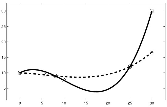
Figure 1. Solid line: Lagrange polynomial; dashed line: piecewise polynomial harmonic (PPH) polynomial. Circles stand for Lagrange values at the nodes, asterisks stand for PPH values at the nodes, and triangles stand for inflection points.

The next experiment computes the numerical approximation order of the considered reconstruction operator.

Let X be a nonuniform grid:

$$X=(\frac{22}{551},\frac{28}{337},\frac{28}{267},\frac{79}{656},\frac{149}{924},\frac{47}{234},\frac{67}{245},\frac{92}{275},\frac{98}{241},\frac{113}{254},\frac{185}{396},\frac{251}{490},\frac{141}{257},\frac{134}{205},\frac{469}{221},\frac{316}{369},\frac{1189}{1259})\pi ,$$

and let $f\left(x\right)=sin\left(x\right)$ be a smooth test function. Let us consider the set of initial points given by $(x_i,f\left(x_i\right)),i=1,...,17.$ In this experiment, we will measure the approximation errors and the numerical order of approximation of the presented PPH reconstruction. The numerical order of approximation $p$ is calculated in an iterative way, just by considering at each new iteration $k,k=1,2,3,4,5,6,7$ a nonuniform grid $X_k$ built from the previous one by introducing a new node in the middle of each two consecutive existing nodes. The error $E_k$ for the $PPH$ reconstruction at each iteration $k$ is calculated as a discrete approximation to ${∥f\left(x\right)-PPH\left(x\right)∥}_{\infty }$, thus evaluating a much denser set of points. Both the errors and the approximation orders $p$ for each iteration are shown in Table 1, where we can see that PPH reconstruction tends to fourth-order accuracy with this smooth concave function, as is expected according to Proposition 1.

Table 1. Approximation errors $E_k$ in the $l_{\infty }$ norm and corresponding approximation orders p obtained after k iterations for the PPH reconstruction with $f\left(x\right)=sin\left(x\right),k=0,1,...,7$.

k	${\mathit{E}}_{\mathit{k}}$	p	k	${\mathit{E}}_{\mathit{k}}$	p
0	4.6114 × 10${}^{-4}$	-	4	1.4165 × 10${}^{-8}$	$3.8226$
1	3.3727 × 10${}^{-5}$	$3.7732$	5	9.4710 × 10${}^{-10}$	$3.9027$
2	2.6009 × 10${}^{-6}$	$3.6968$	6	6.1330 × 10${}^{-11}$	$3.9488$
3	2.0042 × 10${}^{-7}$	$3.6979$	7	3.9035 × 10${}^{-12}$	$3.9737$

Defining $h:=\underset{i=1,\dots ,16}{max}\left\{h_i\right\}$, we use the following formulae to compute the numerical order of approximation p:

$$\begin{array}{ccc}\hfill E_{k-1}& \approx & C{\left({\displaystyle \frac{h}{2^{k-1}}}\right)}^p,\hfill \\ \hfill E_k& \approx & C{\left({\displaystyle \frac{h}{2^k}}\right)}^p.\hfill \end{array}$$

Thus,

$${\displaystyle \frac{E_{k-1}}{E_k}}\approx 2^p\to p\approx {log}_2{\displaystyle \frac{E_{k-1}}{E_k}},k=1,2,3,4,5,6,7.$$

The appropriate behavior of the reconstruction can be checked in Figure 2, where the preservation of the concavity and the accuracy of the approximation can be observed.

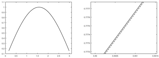
Figure 2. Solid line: function $f\left(x\right)=sin\left(x\right)$; dashed line: PPH reconstruction obtained with the finest considered nonlinear grid. (Left) Original function and PPH reconstruction. (Right) Zoom of a part of the signal.

6. Conclusions

We have defined and studied the PPH reconstruction operator over nonuniform grids, paying special attention to the case of $\sigma$ quasi-uniform grids and initial data coming from strictly convex (concave) underlying functions.

We have theoretically proven some very interesting properties of the new reconstruction operator from the point of view of a potential use in graphical design applications. These properties include the reproduction of polynomials up to the second degree, approximation order, smoothness, boundedness of the operator, Lipschitz continuity, and convexity preservation. In particular, we would like to emphasize the quasi $C^3$ smoothness of the operator and the preservation of strict convexity according to the result contained in Theorem 1.

In the section on the numerical experiments, we checked that the behavior corresponded to the developed theory—in particular, the reconstruction attained fourth-order accuracy and preserved the convexity of the initial data. The results clearly show that the reconstruction introduces improvements in comparison with the Lagrange reconstruction. Therefore, the numerical experiments that we carried out reinforce the theoretical results.

References

- Amat, S.; Donat, R.; Liandrat, J.; Trillo, J.C. Analysis of a new nonlinear subdivision scheme. Applications in image processing. Found. Comput. Math. 2006, 6, 193–225. [Google Scholar] [CrossRef]
- Ortiz, P.; Trillo, J.C. Nonlinear interpolatory reconstruction operator on non uniform grids. arXiv 2018, arXiv:1811.10566. [Google Scholar]
- Amat, S.; Donat, R.; Trillo, J.C. Proving convexity preserving properties of interpolatory subdivision schemes through reconstruction operators. Appl. Math. Comput. 2013, 219, 7413–7421. [Google Scholar] [CrossRef]
- Harten, A. Eno schemes with subcell resolution. J. Comput. Phys. 1989, 83, 148–184. [Google Scholar] [CrossRef]
- Aràndiga, F.; Donat, R. Nonlinear Multi-scale Decomposition: The Approach of A. Harten. Numer. Algorithms 2000, 23, 175–216. [Google Scholar] [CrossRef]
- Amat, S.; Dadourian, K.; Liandrat, J.; Trillo, J.C. High order nonlinear interpolatory reconstruction operators and associated multiresolution schemes. J. Comput. Appl. Math. 2013, 253, 163–180. [Google Scholar] [CrossRef]
- Amat, S.; Liandrat, J. On the stability of PPH nonlinear multiresolution. Appl. Comput. Harmon. Anal. 2005, 18, 198–206. [Google Scholar] [CrossRef]
- Dyn, N.; Gregori, J.A.; Levin, D. A 4-point interpolatory subdivision scheme for curve design. Comput. Aided Geom. Des. 1987, 4, 257–268. [Google Scholar] [CrossRef]
- Dyn, N.; Levin, D. Stationary and non-stationary binary subdivision schemes. Math. Methods Comput. Aided Geom. Des. II 1991, 209–216. Available online: https://doi.org/10.1016/B978-0-12-460510-7.50019-7 (accessed on 3 January 2021).
- Dyn, N.; Kuijt, F.; Levin, D.; Van Damme, R. Convexity preservation of the four-point interpolatory subdivision scheme. Comput. Aided Geom. Des. 1999, 16, 789–792. [Google Scholar] [CrossRef]
- Floater, M.S.; Michelli, C.A. Nonlinear Stationary Subdivision. Approx. Theory 1998, 212, 209–224. [Google Scholar]
- Harten, A. Multiresolution representation of data II. SIAM J. Numer. Anal. 1996, 33, 1205–1256. [Google Scholar] [CrossRef]
- Kuijt, F.; Van Damme, R. Convexity preserving interpolatory subdivision schemes. Constr. Approx. 1998, 14, 609–630. [Google Scholar] [CrossRef]
- Trillo, J.C. Nonlinear Multiresolution and Applications in Image Processing. Ph.D. Thesis, University of Valencia, Valencia, Spain, 2007. [Google Scholar]
Publisher’s Note: MDPI stays neutral with regard to jurisdictional claims in published maps and institutional affiliations. |
© 2021 by the authors. Licensee MDPI, Basel, Switzerland. This article is an open access article distributed under the terms and conditions of the Creative Commons Attribution (CC BY) license (http://creativecommons.org/licenses/by/4.0/).