On the Approximate Solution of Partial Integro-Differential Equations Using the Pseudospectral Method Based on Chebyshev Cardinal Functions

Abstract

In this paper, we apply the pseudospectral method based on the Chebyshev cardinal function to solve the parabolic partial integro-differential equations (PIDEs). Since these equations play a key role in mathematics, physics, and engineering, finding an appropriate solution is important. We use an efficient method to solve PIDEs, especially for the integral part. Unlike when using Chebyshev functions, when using Chebyshev cardinal functions it is no longer necessary to integrate to find expansion coefficients of a given function. This reduces the computation. The convergence analysis is investigated and some numerical examples guarantee our theoretical results. We compare the presented method with others. The results confirm the efficiency and accuracy of the method.

1. Introduction

In this paper, we apply the pseudospectral method based on Chebyshev cardinal functions to solve one-dimensional partial integro-differential equations (PIDEs)

$$w_t(x,t)+\alpha w_{xx}(x,t)=\beta {\int }_0^{t}k(x,t,s,w(x,s))ds+f(x,t),x\in [a,b],t\in [0,T],$$

(1)

with initial and boundary conditions

$$\begin{array}{}\mathrm{(2)}& w(x,0)=g\left(x\right),x\in [a,b],\hfill \mathrm{(3)}& w(0,t)=h_0\left(t\right),w(1,t)=h_1\left(t\right),t\in [0,T],\hfill \end{array}$$

where $\alpha$ and $\beta$ are constants and the functions $f(x,t)$ and $k(x,t,s,w)$ are assumed to be sufficiently smooth on $\mathcal{D}:=[0,1]\times [0,T]$ and $\mathcal{S}$ with $\mathcal{S}:=\left\{\right(x,t,s):x\in [0,1],s,t\in [0,T\left]\right\}$, respectively, as prescribed before and such that (1) has a unique solution $w(x,t)\in C\left(D\right)$. In addition, we assume that the kernel function is of diffusion type which is given by

$$k(x,t,s,w(x,s)):=k_1(x,t-s)w(x,s),$$

(4)

and satisfies the Lipschitz condition as follows

$$\left|k\right(x,t,s,w(x,s))-k(x,t,s,v(x,s))\le \mathcal{A}|w(x,s)-v(x,s)|,$$

(5)

where $\mathcal{A}\ge 0$ is referred to as a Lipschitz constant.

In various fields of physics and engineering, systems are often functions of space and time and are described by partial differential equations. But in some cases, such a formulation can not accurately model this system. Because we can not take into account the effect of a past time when the system is a function of a given time. Such systems appear in heat transfer, thermoelasticity and nuclear reactor dynamics. This phenomenon has resulted in the inclusion of an integral term in the basic partial differential equation that leads to a PIDEs [1]. The existence, uniqueness, and asymptotic behavior of the solution of this equation are discussed in [2]. In this paper, we can find the physical situation that leads to Equation (1). A Simple example that refers to a PIDEs is considered by Habetler and Schiffman [3] where the compression of viscoelastic media is studied. For more applications, we refer readers to [4,5,6,7].

Spectral methods are schemes to discretize the PDEs. To this end, they utilize the polynomials to approximate the exact solution. Since any analytic function can be exponentially approximated by polynomials. In contrast to other methods such as finite elements and finite differences, these methods can achieve an infinite degree of accuracy. That’s mean the order of the convergence of the approximate solution is limited only by the regularity of the exact solution. In other words, for numerical simulations, fewer degrees of freedom are necessary to obtain a given accuracy. The Galerkin method is a class of spectral techniques that convert a continuous operator problem to a discrete problem. In other words, this scheme applies the method of variation of parameters to function space by transforming the equation to a weak formulation. To implement this method, we can not compute the integrals analytically. That’s why we can’t use this method in most cases [8,9]. Another method that is closely related to spectral methods is the pseudospectral method. The pseudospectral methods are a special type of numerical method that used scientific computing and applied mathematics to solve partial differential equations. These methods allow the representation of functions on a quadrature grid and cause simplification of the calculations [10,11].

Several techniques have been used to solve one-dimensional partial differential equations, such as the finite difference method, finite element method, and spectral method. In [12], the Legendre-collocation method is used to solve the parabolic Volterra integro-differential equation. For an infinite domain, Dehghan et al. [12] used the algebraic mapping to obtain a finite domain and then they utilized their proposed method. The Legendre multiwavelets collocation method is used to find the numerical solution of PIDEs [13]. To find the approximate solution of PIDEs, Avazzadeh et al. [14] applied the radial basis functions (RBFs) and finite difference method (FDM). To solve nonlinear parabolic PIDEs in one space variable, Douglas and Jones [15] proposed backward difference and Crank-Nicolson type methods. Han et al. [16] approximated the solution of (1) with kernel function of diffusion type and on unbounded spatial domains using artificial boundary method. In [17], a finite difference scheme is considered to solve PIDEs with a weakly singular kernel.

According to the above, considerable attention has been devoted to solving PIDEs numerically. In this paper, we introduce a simple numerical method with high accuracy. To this end, while introducing the Chebyshev cardinal functions, the pseudospectral method applies to obtain the approximate solution of PIDEs (1). Generally, cardinal functions $\left\{C_i\right\}$ are polynomials of a given degree that $C_i$ vanishes at all interpolation grids except $x_i$. These bases are also called the shape functions, Lagrange basis, and so on. One of the advantages of using such bases is the reduction of calculations to find the expansion coefficients of a given function. In other words, to find the expansion coefficients based on these bases, there is no need to integrate, and this is due to the cardinality, which makes these bases superior to other functions. Laksetani and Dehghan [18] is used Chebyshev cardinal functions to solve a PDE with an unknown time-dependent coefficient. In [19], these functions are used to solve the fractional differential equation. Heydari [20] described a new direct scheme for solving variable-order fractional optimal control problem via Chebyshev cardinal functions. For more details about the Chebyshev cardinal functions and their applications, we refer the reader to [21,22].

This paper is organized as follows, Section 2 is devoted to a brief introduction to Chebyshev cardinal functions. In Section 3, we presented an efficient and applicable method based on Chebyshev cardinal functions to solve PIDEs (1). In Section 4, the convergence analysis is investigated and we proved that the proposed method is convergence. Section 5 is devoted to some numerical tests to show the ability ad accuracy of the method. Finally, Section 6 contains a few concluding remarks.

2. Chebyshev Cardinal Functions

Given $M\in \mathbb{N}$, assume that $\mathcal{M}:=\{1,2,\dots ,M+1\}$ and $\mathcal{X}:=\{x_i:T_{M+1}\left(x_i\right)=0,i\in \mathcal{M}\}$ where $T_{M+1}$ is the first kind Chebyshev function of order $M+1$ on $[-1,1]$. Recall that the Chebyshev grid is obtained by

$$x_i:=cos\left(\frac{(2i-1)\pi }{2M+2}\right),\forall i\in \mathcal{M}.$$

(6)

To utilize the Chebyshev functions of any arbitrary interval $[a,b]$, one can apply the change the variable $x=\left(\frac{2(t-a)}{b-a}-1\right)$ to obtain the shifted Chebyshev functions, viz

$$T_{M+1}^{*}\left(t\right):=T_{M+1}\left(\frac{2(t-a)}{b-a}-1\right),t\in [a,b].$$

(7)

Note that it is easy to show that the grids of shifted Chebyshev function $T_{M+1}^{*}$ is equal to $t_i=\frac{(x+1)(b-a)}{2}+a$.

A significant example of the cardinal functions for orthogonal polynomials is the Chebyshev cardinal functions. The cardinal Chebyshev functions of order $M+1$ are defined as

$$C_i\left(x\right)=\frac{T_{M+1}\left(x\right)}{T_{M+1,x}\left(x_i\right)(x-x_i)},i\in \mathcal{M},$$

(8)

where the subscript x denotes x-differentiation. It is obvious that the functions $C_i\left(x\right)$ are polynomials of degree M which satisfy the condition

$$C_i\left(x_l\right)={\delta }_{il}$$

(9)

where ${\delta }_{il}$ is the Kronecker $\delta$-function.

In view of (9), the cardinal functions are nonzero at one and only one of the points $x_i\in \mathcal{X}$ implies that for arbitrary function $p\left(t\right)$, the function can be approximated by

$$p\left(t\right)\approx \sum _{i=1}^{M+1}p\left(t_i\right)C_i\left(t\right).$$

(10)

Assume that $H^n\left([a,b]\right),n\in \mathbb{N}$ (Sobolev spaces) denotes the space of all functions $p\in C^n\left([a,b]\right)$ such that $D^{\alpha }p\in L^2\left([a,b]\right)$ for all $\alpha \le n$, where $\alpha$ is a nonnegative integer and D is the derivative operator. Sobolov space $H^n\left([a,b]\right)$ is equipped with a norm defined by

$${\parallel p\parallel }_{H^n\left([a,,b]\right)}^2=\sum _{l=0}^n{\parallel p^{\left(l\right)}\left(t\right)\parallel }_{L^2\left([a,b]\right)}^2.$$

(11)

There exista a semi-norm that is defined as follows

$${\left|p\right|}_{H^{n,M}\left([a,b]\right)}^2=\sum _{l=minn,M}^M{\parallel p^{\left(l\right)}\left(t\right)\parallel }_{L^2\left([a,b]\right)}^2.$$

(12)

It follows from [23] that the error of expansion (10) can be bounded by the following lemma.

Lemma 1.

Let ${\left\{t_i\right\}}_{i\in \mathcal{M}}\in {\mathcal{X}}^{*}$ denotes shifted Gauss-Chebyshev points where ${\mathcal{X}}^{*}:=\{t_i:T_{M+1}^{*}\left(t_i\right)=0,i\in \mathcal{M}\}$ and that $p\left(t\right)\in {\mathcal{H}}^n\left([a,b]\right)$ can be approximated by $p_M$ via

$$p_M\left(t\right)=\sum _{i=1}^{M+1}p\left(t_i\right)C_i\left(t\right).$$

Then one can prove that

$$\parallel p-p_M{\parallel }_{L^2\left([a,b]\right)}\le C{M}^{-n}{\left|p\right|}_{H^{n,M}\left([a,b]\right)},$$

(13)

where C is a constant and independent of M.

3. Pseudospectral Method

In this section, we apply the pseudospectral method to solve PIDEs (1) based on Chebyshev cardinal functions. Let us consider the partial integro-differential Equation (1) on the region $\Omega \times \mathrm{T}$. We introduce differential operator

$$\mathcal{L}:=\frac{\partial }{\partial t}+\alpha \frac{{\partial }^2}{\partial x^2},$$

(14)

and integral operator

$$\mathcal{I}:=\beta {\int }_0^{t}k(x,t,s,.)ds.$$

(15)

Applying these operators, PIDEs (1) can be rewritten in the operator form

$$(\mathcal{L}+\mathcal{I})\left(w\right)=f.$$

(16)

Let the solution of (1) is approximated by the polynomial $\tilde{w}(x,t)$, via

$$\tilde{w}(x,t)=\sum _{i=1}^{M+1}\sum _{j=1}^{M+1}{w}^n(t_i,t_j)C_i\left(x\right)C_j\left(t\right).$$

(17)

If we define a matrix W of dimension $(M+1)\times (M+1)$ whose $(i,j)$-th element is $w(t_i,t_j)$, then Equation (17) becomes the matrix problem

$$\tilde{w}(x,t)={\mathcal{C}}^T\left(x\right)W\mathcal{C}\left(t\right),$$

(18)

where the vector elements of $\mathcal{C}\left(x\right)$ are the Chebyshev cardinal functions $\left\{C_i\left(x\right)\right\}$.

Inasmuch as the Chebyshev cardinal functions are polynomial, it is easy to evaluate their derivatives. In view of (17), one can write

$${\tilde{w}}_x(x,t)=\sum _{i=1}^{M+1}\sum _{i=1}^{M+1}w(t_i,t_j)C_{i,x}\left(x\right)C_j\left(t\right)={\mathcal{C}}_x^T\left(x\right)W\mathcal{C}\left(t\right),$$

(19)

where ${\mathcal{C}}_x\left(x\right)$ is a vector of dimension $(M+1)$ whose i-th element is $C_{i,x}\left(x\right)$. Similarly we have

$${\tilde{w}}_t(x,t)=\sum _{i=1}^{M+1}\sum _{i=1}^{M+1}w(t_i,t_j)C_{i,x}\left(x\right)C_j\left(t\right)={\mathcal{C}}^T\left(x\right)W{\mathcal{C}}_t\left(t\right),$$

(20)

where ${\mathcal{C}}_t\left(t\right)$ is a vector of dimension $(M+1)$ whose i-th element is $C_{i,t}\left(t\right)$. Suppose that $\mathcal{D}\in {\mathbb{R}}^{M+1,M+1}$ is the operational matrix of derivative whose $(i,j)$-th element is ${\mathcal{D}}_{i,j}=C_{i,t}\left(t_j\right)$. Thus, it follows from ${\mathcal{C}}_x\left(x\right)=\mathcal{D}\mathcal{C}\left(x\right)$ that

$${\tilde{w}}_x(x,t)={\mathcal{C}}^T\left(x\right){\mathcal{D}}^{T}W\mathcal{C}\left(t\right),$$

(21)

and

$${\tilde{w}}_t(x,t)={\mathcal{C}}^T\left(x\right)W\mathcal{D}\mathcal{C}\left(t\right).$$

(22)

It can easily be shown that ${\tilde{w}}_{xx}(x,t)$ is approximated as follows

$${\tilde{w}}_{xx}(x,t)={\mathcal{C}}^T\left(x\right){{\mathcal{D}}^T}^{2}W\mathcal{C}\left(t\right).$$

(23)

Thus, by substituting (22) and (23) into the differential part of desired Equation (16), we can approximate the differential operator $\mathcal{L}$ (14), via

$$\mathcal{L}\left(w\right)(x,t)\approx {\mathcal{C}}^T\left(x\right)W\mathcal{D}\mathcal{C}\left(t\right)+\alpha {\mathcal{C}}^T\left(x\right){{\mathcal{D}}^T}^{2}W\mathcal{C}\left(t\right),$$

(24)

To approximate the integral part, we assume that

$${\int }_0^t\mathcal{C}\left(x\right)dx=I\mathcal{C}\left(t\right),$$

(25)

where $I\in {\mathbb{R}}^{M+1,M+1}$ is the operational matrix of integral. It follows from (15) that

$$\mathcal{I}\left(w\right)(x,t)=\beta {\int }_0^{t}k(x,t,s,w(x,s))ds.$$

(26)

If we replace w with $\tilde{w}$, then one can write

$$\mathcal{I}\left(w\right)(x,t)\approx \beta {\int }_0^{t}k(x,t,s,\tilde{w}(x,s))ds.$$

(27)

Assume that $k(x,t,s,\tilde{w}(x,s))$ can be approximated by ${\mathcal{C}}^T\left(x\right)K\mathcal{C}\left(t\right)$ where K is a matrix whose elements depend on t and unknown coefficients W. Replacing ${\mathcal{C}}^T\left(x\right)K\mathcal{C}\left(t\right)$ into (27), and using the operational matrix of integration I, we get

$$\begin{array}{cc}\hfill \mathcal{I}\left(w\right)(x,t)& \approx \beta {\int }_0^t{\mathcal{C}}^T\left(x\right)K\mathcal{C}\left(s\right)ds\hfill \\ \hfill & =\beta {\mathcal{C}}^T\left(x\right)K{\int }_0^t\mathcal{C}\left(s\right)ds\hfill \\ \hfill & =\beta {\mathcal{C}}^T\left(x\right)KI\mathcal{C}\left(t\right)\hfill \\ \hfill & =q(x,t)={\mathcal{C}}^T\left(x\right)Q\mathcal{C}\left(t\right),\hfill \end{array}$$

(28)

where $(i,j)$-th element of matrix Q is $q(t_i,t_j)$. Substituting (25) and (28) into (16), one can write

$${\mathcal{C}}^T\left(x\right)(W\mathcal{D}+\alpha {{\mathcal{D}}^T}^{2}W+Q)\mathcal{C}\left(t\right)={\mathcal{C}}^T\left(x\right)F\mathcal{C}\left(t\right).$$

(29)

The Chebyshev cardinal functions $\left\{C_i\left(x\right)\right\}$ are orthogonal with respect to weighted inner product on $[-1,1]$

$${⟨C_i\left(x\right),C_j\left(x\right)⟩}_{\omega \left(x\right)}=\left\{\begin{array}{cc}\frac{\pi }{M+1},\hfill & i=j,\hfill \\ 0,\hfill & i\ne j,\hfill \end{array}\right.$$

where $\omega \left(x\right)=1/\sqrt{1-x^2}$. This gives rise to equation

$$W\mathcal{D}+\alpha {{\mathcal{D}}^T}^{2}W+Q=F.$$

(30)

Let us rewrite this system as

$$\mathcal{F}\left(W\right):=W\mathcal{D}+\alpha {{\mathcal{D}}^T}^{2}W+Q-F=0.$$

(31)

We Replace the first column of (31) with the initial condition (2) and the first and last rows of (31) with the boundary conditions (3), i.e.,

$$\begin{array}{cc}\hfill {\left[\mathcal{F}\left(W\right)\right]}_{i,1}& ={\left[W\mathcal{C}\left(0\right)\right]}_i-g\left(t_i\right),\hfill \\ \hfill {\mathcal{F}\left(W\right)]}_{1,i}& ={\left[{\mathcal{C}}^T\left(0\right)W\right]}_i-h_0\left(t_i\right),\hfill \\ \hfill {\mathcal{F}\left(W\right)]}_{M+1,i}& ={\left[{\mathcal{C}}^T\left(1\right)W\right]}_i-h_1\left(t_i\right),\hfill \\ \hfill i=1,\dots ,M+1.\end{array}$$

Using the matrix to vector conversion, this system is changed to a new system by ${(M+1)}^2$ equations with ${(M+1)}^2$ unknowns

$$\left\{\begin{array}{cc}\overline{W}\Gamma =\mathfrak{F},\hfill & \mathrm{if} k \mathrm{is} a \mathrm{nonlinear} \mathrm{function} \mathrm{of} w,\hfill \\ \overline{\mathcal{F}}=\mathfrak{F},\hfill & \mathrm{if} k \mathrm{is} a \mathrm{linear} \mathrm{function} \mathrm{of} w,\hfill \end{array}\right.$$

(32)

where $\overline{W}$, $\mathfrak{F}$, and $\overline{\mathcal{F}}$ are obtained using the matrix to vector conversion of W, F, and $\mathcal{F}$ respectively.

After solving the linear or nonlinear system (32) using the generalized minimal residual method (GMRES) [24] and Newton-Raphson method, respectively, the unknowns W are found, and then the approximate solution can be obtained using (18).

4. Convergence Analysis

Because the function $f(x,t)$ is a continuous function on D, the approximate error by comparing the function f with $\tilde{f}$ may be bounded, established by the following theorem.

Theorem 1.

Let $f:D\to {\mathbb{R}}^2$ be a sufficiently smooth function. Thus Chebyshev cardinal approximation to function f can be written as

$$\parallel f-\tilde{f}\parallel \approx O\left(2^{-2M}\right).$$

(33)

Proof. 

Let $P_{M+1}\left(x\right)$ denote that polynomial of degree $M+1$ which interpolates to the function f at the $M+1$ zeros of the first kind Chebyshev polynomials. It follows from [25] that

$$\begin{array}{cc}\hfill |f(x,t)-P_{M+1}(x,t)|& =\frac{{\partial }^{M+1}}{\partial x^{M+1}}f(\xi ,t)\frac{{\Pi }_{i=1}^{M+1}(x-t_i)}{(M+1)!}+\frac{{\partial }^{M+1}}{\partial t^{M+1}}f(x,\eta )\frac{{\Pi }_{j=1}^{M+1}(t-t_j)}{(M+1)!}\hfill \\ \hfill & -\frac{{\partial }^{2M+2}}{\partial x^{M+1}{t}^{M+1}}f({\xi }^{\prime },{\eta }^{\prime })\frac{{\Pi }_{i=1}^{M+1}(x-t_i){\Pi }_{j=1}^{M+1}(t-t_j)}{(M+1)!(M+1)!}.\hfill \end{array}$$

Since the leading coefficient of the first kind Chebyshev functions is $2^M$, and $|T_i\left(x\right)|\le 1$, $\forall i\in \mathcal{M}$. It is possible to write

$$\begin{array}{cc}\hfill |f(x,t)-P_{M+1}(x,t)|& \le {\left(\frac{b-a}{2}\right)}^{M+1}\frac{1}{2^M(M+1)!}\left(\underset{\xi \in [a,b]}{sup}|\frac{{\partial }^{M+1}}{\partial x^{M+1}}f(\xi ,t)|+\underset{\eta \in [0,T]}{sup}\left|\frac{{\partial }^{M+1}}{\partial t^r}f(x,\eta )\right|\right)\hfill \\ \hfill & +{\left(\frac{b-a}{2}\right)}^{2M+2}\frac{1}{4^M{((M+1)!)}^2}\underset{({\xi }^{\prime },{\eta }^{\prime })\in D}{sup}\left|\frac{{\partial }^{2M+2}}{\partial x^r\partial t^{M+1}}f({\xi }^{\prime },{\eta }^{\prime })\right|.\hfill \end{array}$$

Since $\tilde{f}$ is approximated by Chebyshev cardinal functions and these bases are polynomials, thus one can obtain

$$\begin{array}{cc}\hfill \parallel f-\tilde{f}{\parallel }^2& ={\int \int }_D{|f(x,t)-\tilde{f}(x,t)|}^{2}dtdx\hfill \\ \hfill & \le {\int \int }_D{|f(x,t)-P_{M+1}(x,t)|}^{2}dtdx\hfill \\ \hfill & \le {\int \int }_D{\left(\frac{b-a}{2}\right)}^{M+1}\frac{1}{2^M(M+1)!}\left(\underset{\xi \in [a,b]}{sup}|\frac{{\partial }^{M+1}}{\partial x^{M+1}}f(\xi ,t)|+\underset{\eta \in [0,T]}{sup}\left|\frac{{\partial }^{M+1}}{\partial t^r}f(x,\eta )\right|\right)dtdx\hfill \\ \hfill & +{\int \int }_D{\left(\frac{b-a}{2}\right)}^{2M+2}\frac{1}{4^M{((M+1)!)}^2}\underset{({\xi }^{\prime },{\eta }^{\prime })\in D}{sup}\left|\frac{{\partial }^{2M+2}}{\partial x^r\partial t^{M+1}}f({\xi }^{\prime },{\eta }^{\prime })\right|dtdx\hfill \\ \hfill & \le 2^{-2M}\frac{{(b-a)}^{2M}}{(M+1)!}{\mathcal{C}}_{max}(1/2+2^{-2M-2}/(M+1)!)\underset{D}{\int \int }dtdx\hfill \\ \hfill & \le {\mathcal{C}}_1{2}^{-2M},\hfill \end{array}$$

where ${\mathcal{C}}_1:=\frac{{(b-a)}^{2M}}{(M+1)!}{\mathcal{C}}_{max}(1/2+2^{-2M-2}/(M+1)!)\left|D\right|$ and

$${\mathcal{C}}_{max}:=max\{\underset{\xi \in [a,b]}{sup}|\frac{{\partial }^{M+1}}{\partial x^{M+1}}f(\xi ,t)|,\underset{\eta \in [0,T]}{sup}|\frac{{\partial }^{M+1}}{\partial t^r}|,\underset{({\xi }^{\prime },{\eta }^{\prime })\in D}{sup}|\frac{{\partial }^{2M+2}}{\partial x^r\partial t^{M+1}}\left|\right\}.$$

 □

Theorem 2.

The pseudospectral method for solving PIDEs (1) is convergence.

Proof. 

Let $\tilde{w}$ denotes the approximate solution of (1) for which $e=w-\tilde{w}$. We subtract Equation (1) from

$${\tilde{w}}_t(x,t)+\alpha {\tilde{w}}_{xx}(x,t)=\beta {\int }_0^{t}k(x,t,s,\tilde{w}(x,s))ds+\tilde{f}(x,t),$$

(34)

to obtain the following equation

$$e_t(x,t)+\alpha e_{xx}(x,t)=\beta {\int }_0^{t}k(x,t,s,e(x,s))ds+f(x,t)-\tilde{f}(x,t).$$

(35)

Now, Assume that we can approximate the error function $e(x,t)$ as follows

$$e(x,t)\approx {\mathcal{C}}^T\left(x\right)E\mathcal{C}\left(t\right),$$

(36)

where E is a matrix whose $(i,j)$-th element is $e(t_i,t_j)$. Using this approximation and Lipschitz condition (5), Equation (35) may be written as

$${\mathcal{C}}^T\left(x\right)E\mathcal{D}\mathcal{C}\left(t\right)+\alpha {\mathcal{C}}^T\left(x\right){{\mathcal{D}}^T}^{2}E\mathcal{C}\left(t\right)\le \beta \mathcal{A}{\mathcal{C}}^T\left(x\right)EI\mathcal{C}\left(t\right)+{\mathcal{C}}^T\left(x\right)\eta \mathcal{C}\left(t\right),$$

(37)

where $|f-\tilde{f}|\approx {\mathcal{C}}^T\left(x\right)\eta \mathcal{C}\left(t\right)$. By dropping the second term in the left to the other side of the inequality and taking norm from both sides, we have

$$\parallel E\mathcal{D}\parallel \le \mathcal{A}\left|\beta \right|\parallel EI\parallel +\left|\alpha \right|\parallel {{\mathcal{D}}^T}^{2}E\parallel +\parallel \eta \parallel .$$

(38)

Because $\left\{C_i\right\}$ are orthogonal functions, we removed $\parallel \mathcal{C}\parallel$ from both sides. Multiplying the right side of (38) by $\parallel \mathcal{D}\parallel$, it follows that

$$\begin{array}{cc}\hfill \parallel E\mathcal{D}\parallel & \le \mathcal{A}\left|\beta \right|\parallel EI\parallel \parallel \mathcal{D}\parallel +\left|\alpha \right|\parallel {{\mathcal{D}}^T}^{2}E\parallel \parallel \mathcal{D}\parallel +\parallel \eta \parallel \parallel \mathcal{D}\parallel \hfill \\ \hfill & \le \mathcal{A}\left|\beta \right|\parallel E\parallel \parallel I\parallel \parallel \mathcal{D}\parallel +\left|\alpha \right|\parallel {{\mathcal{D}}^T}^2\parallel \parallel E\parallel \parallel \mathcal{D}\parallel +\parallel \eta \parallel \parallel \mathcal{D}\parallel ,\hfill \end{array}$$

and then

$$\begin{array}{cc}\hfill \parallel E\parallel \parallel \mathcal{D}\parallel & \le \mathcal{A}\left|\beta \right|\parallel EI\parallel \parallel \mathcal{D}\parallel +\left|\alpha \right|\parallel {{\mathcal{D}}^T}^{2}E\parallel \parallel \mathcal{D}\parallel +\parallel \eta \parallel \parallel \mathcal{D}\parallel \hfill \\ \hfill \Rightarrow \parallel E\parallel & \le \mathcal{A}\left|\beta \right|\parallel E\parallel \parallel I\parallel +\left|\alpha \right|\parallel {{\mathcal{D}}^T}^2\parallel \parallel E\parallel +\parallel \eta \parallel .\hfill \end{array}$$

So, it is obvious that we shall have

$$\parallel E\parallel \left|1-\mathcal{A}\left|\beta \right|\parallel I\parallel -\left|\alpha \right|\parallel {\mathcal{D}}^2\parallel \right|\le \parallel \eta \parallel .$$

(39)

Consequently, we obtain

$$\parallel E\parallel \le {\left|1-\mathcal{A}\left|\beta \right|\parallel I\parallel -\left|\alpha \right|\parallel {\mathcal{D}}^2\parallel \right|}^{-1}\parallel \eta \parallel .$$

(40)

If f be a sufficiently smooth function, then $\parallel \eta \parallel \to 0$ as $M\to \infty$. Thus, we have

$$\parallel e\parallel \to 0,asM\to \infty .$$

Therefore, the proposed method is convergent.  □

5. Test Problems

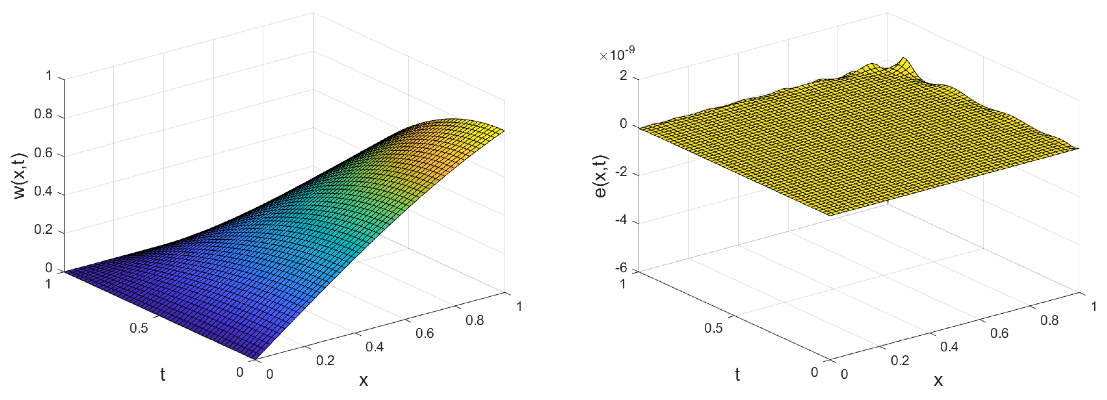
Example 1.

Let us dedicate the first example to the case that the desired Equation (1) is of form

$$w_t(x,t)-w_{xx}(x,t)=f(x,t)-{\int }_0^t{e}^{x(t-s)}w(x,s)ds,$$

with initial and boundary conditions

$$\begin{array}{cc}\hfill w(x,0)& =0,x\in [0,1],\hfill \\ \hfill w(0,t)& =sin\left(t\right),w(1,t)=0,t\in [0,1],\hfill \end{array}$$

and also $f(x,t):=\frac{\left(-x^2+1\right){\mathrm{e}}^{xt}+\left(x^3+2x^2-x+2\right)sin\left(t\right)+\left(-x^4+x^2\right)cos\left(t\right)}{x^2+1}$. The exact solution for this example is given by [13]

$$w(x,t)=(1-x^2)sin\left(t\right).$$

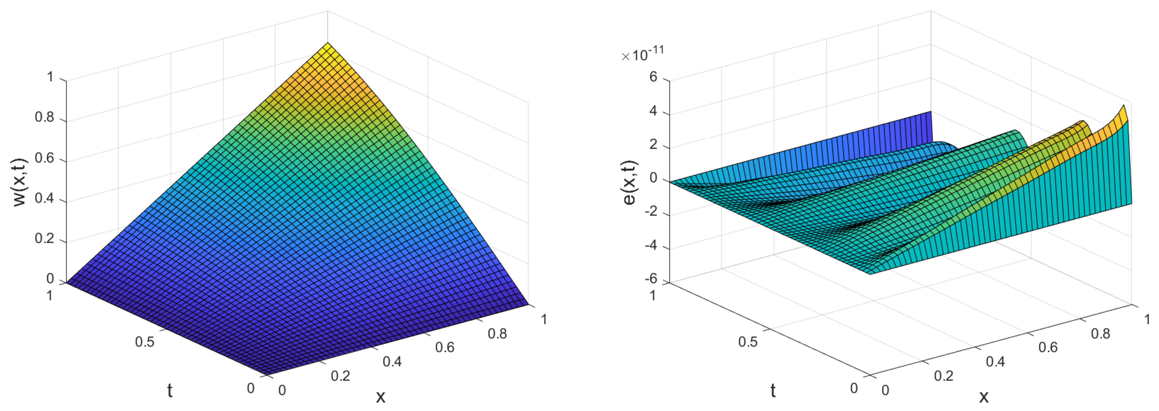
Table 1 shows a comparison between the proposed method and Legendre multiwavelets collocation method [13]. As you can see, our proposed method gives better results than [13]. According to Table 1, we can see that with fewer bases, we have achieved much better accuracy than the method in [13]. For different values of M, the errors in Table 2 are given with $L^{\infty }$, $L^2$ norms applying pseudospectral method based on Chebyshev cardinal functions. In Figure 1, the approximate solution, and absolute value of error are depicted.

Table 1. Comparison of the maximum absolute errors at different times for Example 1.

	Legendre Multiwavelets Collocation Method [13]			Proposed Method
t	$\mathit{M}=8$	$\mathit{M}=16$	$\mathit{M}=32$	$\mathit{M}=8$
$0.0625$	$7.4383\times {10}^{-5}$	$4.6240\times {10}^{-6}$	$1.2106\times {10}^{-5}$	$2.2070\times {10}^{-8}$
$0.1875$	$7.5155\times {10}^{-5}$	$1.2275\times {10}^{-5}$	$2.4685\times {10}^{-5}$	$1.1514\times {10}^{-9}$
$0.3125$	$1.4643\times {10}^{-4}$	$2.5696\times {10}^{-5}$	$3.5745\times {10}^{-5}$	$4.8570\times {10}^{-8}$
$0.4375$	$7.5929\times {10}^{-5}$	$4.2169\times {10}^{-5}$	$4.5563\times {10}^{-5}$	$1.4616\times {10}^{-9}$
$0.5625$	$1.2180\times {10}^{-4}$	$6.0743\times {10}^{-5}$	$5.3926\times {10}^{-5}$	$1.7855\times {10}^{-9}$
$0.6875$	$1.0567\times {10}^{-4}$	$8.1933\times {10}^{-5}$	$6.0499\times {10}^{-5}$	$1.0870\times {10}^{-7}$
$0.8125$	$4.7215\times {10}^{-5}$	$1.0738\times {10}^{-4}$	$6.4915\times {10}^{-5}$	$5.3619\times {10}^{-9}$
$0.9375$	$2.1869\times {10}^{-4}$	$1.3833\times {10}^{-4}$	$6.6396\times {10}^{-5}$	$3.8717\times {10}^{-7}$

Table 2. The $L^{\infty }$, $L^2$ errors and CPU time for Example 1.

m	$\mathit{M}=4$	$\mathit{M}=5$	$\mathit{M}=6$	$\mathit{M}=7$	$\mathit{M}=8$	$\mathit{M}=9$	$\mathit{M}=10$
${\parallel E\parallel }_2$	$5.8921\times {10}^{-3}$	$1.0990\times {10}^{-3}$	$5.7105\times {10}^{-5}$	$3.2074\times {10}^{-6}$	$6.3119\times {10}^{-8}$	$4.6636\times {10}^{-9}$	$7.3474\times {10}^{-11}$
${\parallel E\parallel }_{\infty }$	$5.4300\times {10}^{-2}$	$1.9000\times {10}^{-3}$	$1.1000\times {10}^{-3}$	$1.3510\times {10}^{-4}$	$3.8717\times {10}^{-7}$	$2.3385\times {10}^{-8}$	$3.8785\times {10}^{-10}$
CPU time	$1.141$	$1.985$	$3.953$	$7.172$	$15.890$	$23.515$	$42.031$
Order of convergence	-	-	$1.00679$	$1.10766$	$1.24750$	$1.27087$	$1.33619$

Figure 1. Plot of the approximate solution and absolute value of the error for Example 1.

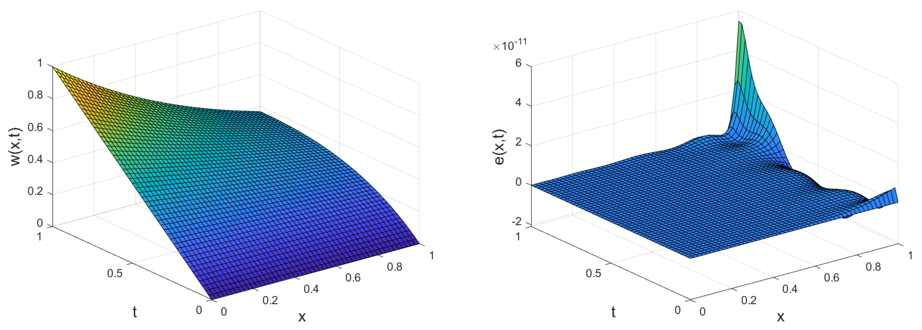
Example 2.

Consider the following PIDEs [14]

$$w_t(x,t)+w_{xx}(x,t)=\frac{\left(-x^3+\left(t^2+1\right)x^2-{\left(t+1\right)}^{2}x+2t\right){\mathrm{e}}^{-xt}+{\mathrm{e}}^{-t}x}{x-1}-{\int }_0^t{e}^{s-t}w(x,s)ds,$$

with initial and boundary conditions

$$\begin{array}{cc}\hfill w(x,0)& =x,x\in [0,1],\hfill \\ \hfill w(0,t)& =0,w(1,t)=e^{-t},t\in [0,1],\hfill \end{array}$$

The exact solution for this example is $w(x,t)=x{e}^{-xt}$.

In Table 3, we report the $L^{\infty }$, $L^2$ errors and CPU time for different values of M. These results guarantee our convergence investigation in Section 4. When M increases, the error decreases, and approaches zero. The $L^{\infty }$, $L^2$ errors obtained by presented method are compared with Hermite-Taylor matrix method [26] and radial basis functions [14] in Table 4. According to Table 4, we can see that our presented method is better than Hermite-Taylor matrix method [26] and radial basis functions [14]. Finally, we illustrate the approximate solution and absolute error in Figure 2.

Table 3. The $L^{\infty }$, $L^2$ errors and CPU time for Example 2.

m	$\mathit{M}=4$	$\mathit{M}=5$	$\mathit{M}=6$	$\mathit{M}=7$	$\mathit{M}=8$	$\mathit{M}=9$	$\mathit{M}=10$
${\parallel E\parallel }_2$	$7.4563\times {10}^{-4}$	$4.7516\times {10}^{-5}$	$3.0177\times {10}^{-6}$	$2.3288\times {10}^{-7}$	$3.4667\times {10}^{-9}$	$2.7823\times {10}^{-10}$	$2.4512\times {10}^{-12}$
${\parallel E\parallel }_{\infty }$	$5.8000\times {10}^{-3}$	$1.1697\times {10}^{-4}$	$2.6094\times {10}^{-5}$	$6.7272\times {10}^{-8}$	$5.0805\times {10}^{-8}$	$1.74111\times {10}^{-9}$	$5.4471\times {10}^{-11}$
CPU time	$0.922$	$1.890$	$3.578$	$6.547$	$15.203$	$23.344$	$40.062$
Order of convergence	-	-	$1.19642$	$1.17133$	$1.29749$	$1.30468$	$1.38764$

Table 4. Comparison of the $L^{\infty }$ and $L^2$ errors at different times for Example 2.

	Reference [14] (M = 12)		Reference [26] (M = 40)		Proposed Method (M = 10)
$\mathit{t}$	${\mathit{L}}^{\mathbf{2}}$-Error	${\mathit{L}}^{\infty }$-Error	${\mathit{L}}^{\mathbf{2}}$-Error	${\mathit{L}}^{\infty }$-Error	${\mathit{L}}^{\mathbf{2}}$-Error	${\mathit{L}}^{\infty }$-Error
$0.1$	$7.9401\times {10}^{-8}$	$3.9522\times {10}^{-8}$	$1.8818\times {10}^{-5}$	$1.1285\times {10}^{-5}$	$8.6171\times {10}^{-15}$	$6.0890\times {10}^{-15}$
$0.2$	$6.7287\times {10}^{-8}$	$3.2388\times {10}^{-8}$	$2.6480\times {10}^{-5}$	$1.6630\times {10}^{-5}$	$1.9171\times {10}^{-14}$	$8.9706\times {10}^{-14}$
$0.3$	$5.8151\times {10}^{-8}$	$2.6768\times {10}^{-8}$	$3.0188\times {10}^{-5}$	$1.9483\times {10}^{-5}$	$3.4101\times {10}^{-14}$	$4.2781\times {10}^{-14}$
$0.4$	$5.1314\times {10}^{-8}$	$2.3917\times {10}^{-8}$	$3.1915\times {10}^{-5}$	$2.0935\times {10}^{-5}$	$4.7705\times {10}^{-14}$	$6.2679\times {10}^{-14}$
$0.5$	$4.6268\times {10}^{-8}$	$2.3437\times {10}^{-8}$	$3.2470\times {10}^{-5}$	$2.1539\times {10}^{-5}$	$1.4383\times {10}^{-13}$	$3.5485\times {10}^{-13}$
$0.6$	$4.2620\times {10}^{-8}$	$2.3220\times {10}^{-8}$	$3.2421\times {10}^{-5}$	$2.1615\times {10}^{-5}$	$2.9489\times {10}^{-13}$	$4.3306\times {10}^{-13}$
$0.7$	$4.0062\times {10}^{-8}$	$2.3226\times {10}^{-8}$	$3.2001\times {10}^{-5}$	$2.1366\times {10}^{-5}$	$5.3306\times {10}^{-13}$	$7.6451\times {10}^{-13}$
$0.8$	$3.8392\times {10}^{-8}$	$2.3424\times {10}^{-8}$	$3.1393\times {10}^{-5}$	$2.0923\times {10}^{-5}$	$9.3758\times {10}^{-13}$	$1.3921\times {10}^{-12}$
$0.9$	$3.7575\times {10}^{-8}$	$2.3788\times {10}^{-8}$	$3.0699\times {10}^{-5}$	$2.0376\times {10}^{-5}$	$1.3326\times {10}^{-12}$	$1.3917\times {10}^{-12}$

Figure 2. Plot of the approximate solution and absolute value of the error for Example 2.

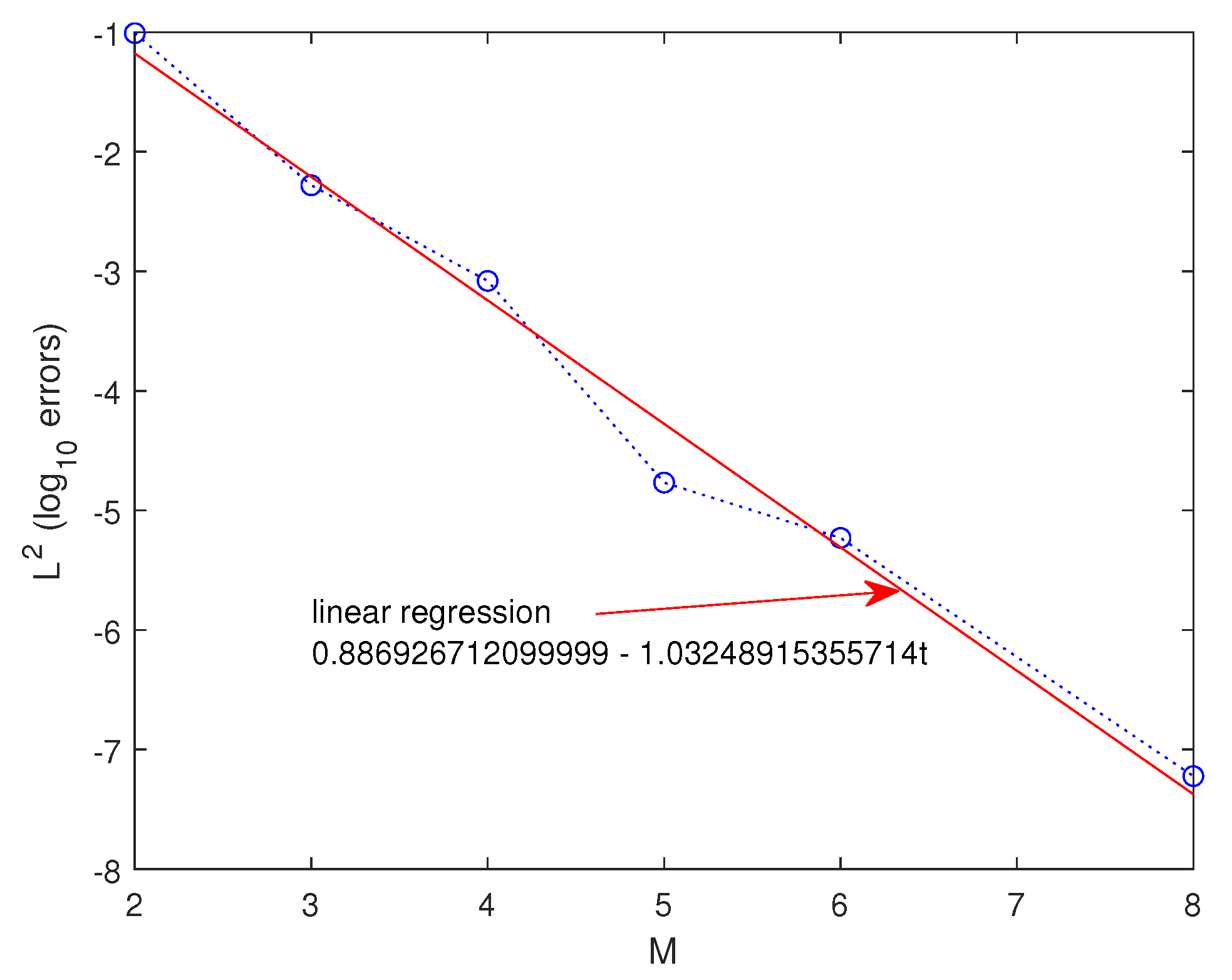
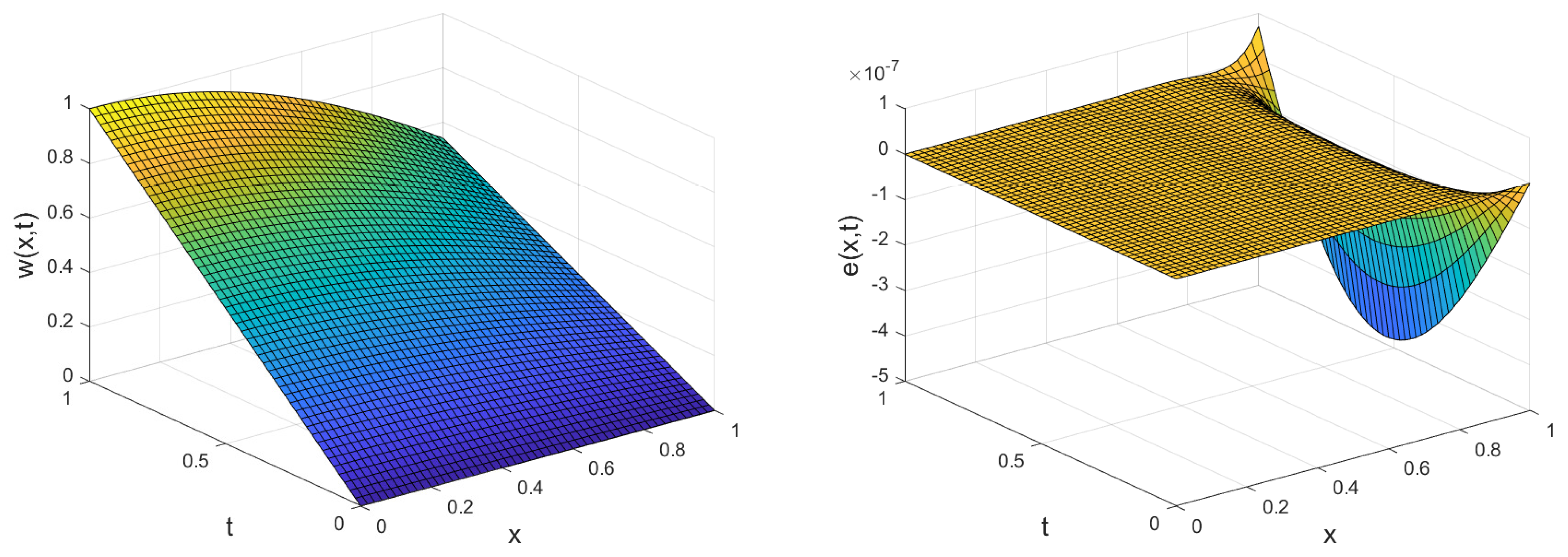
Example 3.

To show the ability of the proposed method for solving nonlinear PIDEs (1), we consider the following equation.

$$w_t(x,t)+w_{xx}(x,t)={\int }_0^t{e}^{x+t+s}{w}^2(x,s)+f(x,t),$$

where

$$f(x,t)=\frac{\left(x\left({\left(cos\left(t\right)\right)}^2+2cos\left(t\right)sin\left(t\right)+2\right){\mathrm{e}}^{x+2t}-3{\mathrm{e}}^{x+t}x-5sin\left(t\right)\right)x}{5},$$

with the boundary and initial conditions

$$\begin{array}{cc}\hfill w(x,0)& =x,x\in [0,1],\hfill \\ \hfill w(0,t)& =0,w(1,t)=cos\left(t\right),t\in [0,1],\hfill \end{array}$$

The exact solution for this Example is given by $w(x,t):=xcos\left(t\right)$. Thus, we can easily judge the accuracy and convergency of the method.

Figure 3 illustrates the $log\left(L^{2}errors\right)$, taking different values for M. To show the order of convergence, we also plotted the linear regression. The slope of this line is equal to the order of convergence $\left(1.03248915355714\right)$. The numerical values with associated $L^2$ error and $L^{\infty }$ error are tabulated in Table 5. Finally, we illustrate the approximate solution and absolute error, taking $M=8$ in Figure 4.

Figure 3. Plot of the $log\left(L^{2}errors\right)$ and the linear regression for Example 3.

Table 5. The $L^{\infty }$ and $L^2$ errors for Example 3.

m	$\mathit{M}=2$	$\mathit{M}=3$	$\mathit{M}=4$	$\mathit{M}=5$	$\mathit{M}=6$	$\mathit{M}=7$	$\mathit{M}=8$
${\parallel E\parallel }_2$	$9.8128\times {10}^{-2}$	$5.2408\times {10}^{-3}$	$8.3112\times {10}^{-4}$	$1.7116\times {10}^{-5}$	$5.8815\times {10}^{-6}$	$6.8421\times {10}^{-7}$	$6.0015\times {10}^{-8}$
${\parallel E\parallel }_{\infty }$	$3.8674\times {10}^{-1}$	$2.9204\times {10}^{-2}$	$7.7564\times {10}^{-3}$	$2.6865\times {10}^{-4}$	$3.9205\times {10}^{-5}$	$6.2192\times {10}^{-6}$	$4.8173\times {10}^{-7}$

Figure 4. Plot of the approximate solution and absolute value of the error for Example 3.

Example 4.

The last example is dedicated to equation

$$w_t(x,t)-w_{xx}(x,t)=f(z,t)+{\int }_0^{t}3xst{e}^{w(x,s)}ds,$$

where

$$f(x,t):=\frac{-3t^{2}xcos\left(sin\left(x\right)t\right)sin\left(x\right)+3txsin\left(sin\left(x\right)t\right)-sin\left(x\right)\left(cos\left(x\right)-1\right)\left(cos\left(x\right)+1\right)\left(t+1\right)}{{\left(sin\left(x\right)\right)}^2},$$

and

$$\begin{array}{cc}\hfill w(x,0)& =0,x\in [0,1],\hfill \\ \hfill w(0,t)& =0,w(1,t)=sin\left(1\right)t,t\in [0,1],\hfill \end{array}$$

Since the closed form of the exact solution to the problem is unavailable, we compute a reference solution by picking a large $M=12$. The $L^{\infty }$, $L^2$ errors, CPU time and order of convergence are tabulated in Table 6 for different values of M. Figure 5 illustrates the approximate solution and absolute error, taking $M=9$. Table 7 shows the $L^{\infty }$, $L^2$ errors at the different times, taking different M.

Table 6. The $L^{\infty }$, $L^2$ errors, CPU time and order of convergence for Example 4.

m	$\mathit{M}=3$	$\mathit{M}=4$	$\mathit{M}=5$	$\mathit{M}=6$	$\mathit{M}=7$	$\mathit{M}=8$	$\mathit{M}=9$
${\parallel E\parallel }_2$	$3.9186\times {10}^{-2}$	$1.3828\times {10}^{-4}$	$9.8169\times {10}^{-6}$	$3.2073\times {10}^{-7}$	$1.5216\times {10}^{-8}$	$3.7417\times {10}^{-10}$	$1.3539\times {10}^{-11}$
${\parallel E\parallel }_{\infty }$	$6.3472\times {10}^{-4}$	$7.3752\times {10}^{-6}$	$2.8966\times {10}^{-6}$	$7.4561\times {10}^{-8}$	$3.2107\times {10}^{-9}$	$1.5876\times {10}^{-11}$	$2.3226\times {10}^{-12}$
CPU time	$0.750$	$1.203$	$2.547$	$4.640$	$8.656$	$27.703$	$34.516$
Order of convergence	-	-	$1.73646$	$1.60251$	$1.51998$	$1.50915$	$1.49803$

Figure 5. Plot of the approximate solution and absolute value of the error for Example 4.

Table 7. Comparison of the $L^{\infty }$ and $L^2$ errors at different times for Example 4.

	M = 6		M = 8		M = 10
$\mathit{t}$	${\mathit{L}}^{\mathbf{2}}$-Error	${\mathit{L}}^{\infty }$-Error	${\mathit{L}}^{\mathbf{2}}$-Error	${\mathit{L}}^{\infty }$-Error	${\mathit{L}}^{\mathbf{2}}$-Error	${\mathit{L}}^{\infty }$-Error
$0.1$	$3.6577\times {10}^{-8}$	$7.4561\times {10}^{-8}$	$4.3201\times {10}^{-11}$	$5.8656\times {10}^{-11}$	$3.0868\times {10}^{-14}$	$4.9832\times {10}^{-14}$
$0.2$	$8.9209\times {10}^{-8}$	$1.7000\times {10}^{-7}$	$1.0306\times {10}^{-10}$	$1.4755\times {10}^{-10}$	$7.3013\times {10}^{-14}$	$1.1669\times {10}^{-13}$
$0.3$	$1.4797\times {10}^{-7}$	$2.6555\times {10}^{-7}$	$1.7008\times {10}^{-10}$	$2.4742\times {10}^{-10}$	$1.2171\times {10}^{-13}$	$1.9019\times {10}^{-13}$
$0.4$	$2.0766\times {10}^{-7}$	$3.5705\times {10}^{-7}$	$2.4193\times {10}^{-10}$	$3.5170\times {10}^{-10}$	$1.7217\times {10}^{-13}$	$2.6485\times {10}^{-13}$
$0.5$	$2.6816\times {10}^{-7}$	$4.4936\times {10}^{-7}$	$3.1506\times {10}^{-10}$	$4.5674\times {10}^{-10}$	$2.2295\times {10}^{-13}$	$3.3922\times {10}^{-13}$
$0.6$	$3.3127\times {10}^{-7}$	$5.4884\times {10}^{-7}$	$3.8600\times {10}^{-10}$	$5.6010\times {10}^{-10}$	$2.7508\times {10}^{-13}$	$4.1582\times {10}^{-13}$
$0.7$	$3.9738\times {10}^{-7}$	$6.5574\times {10}^{-7}$	$4.5574\times {10}^{-10}$	$6.6222\times {10}^{-10}$	$3.2645\times {10}^{-13}$	$4.9100\times {10}^{-13}$
$0.8$	$4.6191\times {10}^{-7}$	$7.5670\times {10}^{-7}$	$5.2929\times {10}^{-10}$	$7.6617\times {10}^{-10}$	$3.7527\times {10}^{-13}$	$5.6141\times {10}^{-13}$
$0.9$	$5.1196\times {10}^{-7}$	$8.1715\times {10}^{-7}$	$6.0246\times {10}^{-10}$	$8.7071\times {10}^{-10}$	$4.2776\times {10}^{-13}$	$6.3991\times {10}^{-13}$
$1.0$	$5.2605\times {10}^{-7}$	$8.0354\times {10}^{-7}$	$6.3088\times {10}^{-10}$	$9.5150\times {10}^{-10}$	$4.5370\times {10}^{-13}$	$6.7249\times {10}^{-13}$

6. Conclusions

In this paper, an efficient and novel numerical method is applied to solve partial integro-differential equations using the pseudospectral method based on Chebyshev cardinal functions. Due to the simplicity of using cardinal functions, the presented method is good for solving PIDEs. The convergence analysis is investigated and we can show when the number of bases increases, the accuracy is also increased. The presented method was applied to solve some numerical tests and the results guarantee our convergence investigation and application of the proposed method to this problem shows that it performs extremely well in terms of accuracy.