A New Goodness of Fit Test for Multivariate Normality and Comparative Simulation Study

Abstract

The testing of multivariate normality remains a significant scientific problem. Although it is being extensively researched, it is still unclear how to choose the best test based on the sample size, variance, covariance matrix and others. In order to contribute to this field, a new goodness of fit test for multivariate normality is introduced. This test is based on the mean absolute deviation of the empirical distribution density from the theoretical distribution density. A new test was compared with the most popular tests in terms of empirical power. The power of the tests was estimated for the selected alternative distributions and examined by the Monte Carlo modeling method for the chosen sample sizes and dimensions. Based on the modeling results, it can be concluded that a new test is one of the most powerful tests for checking multivariate normality, especially for smaller samples. In addition, the assumption of normality of two real data sets was checked.

1. Introduction

Much multivariate data is being collected by monitoring natural and social processes. IBM estimates that we all generate 175 zettabytes of data every day. To add, the data were collected at a rapidly increasing rate, i.e., it is estimated that 90% of data has been generated in the last two years. The need to extract useful information from continuously generated data sets drives demand for data specialists and the development of robust analysis methods.

Data analytics is inconceivable without testing the goodness of fit hypothesis. The primary task of a data analyst is to become familiar with the data sets received. This usually starts by identifying the distribution of the data. Then, the assumption that the data follow a normal distribution is usually tested. Since 1990, many tests have been developed to test this assumption, mostly for univariate data.

It is important to use the powerful tests for the goodness of fit hypothesis to test the assumption of normality because an alternative distribution is not known in general. Based on the outcome of normality verification, one can choose suitable analysis methods (parametric or non-parametric) for further investigation. From the end of the 20th century to the present day, multivariate tests for testing the goodness of fit hypothesis have been developed by a number of authors [1,2,3,4,5,6,7,8,9,10,11,12,13,14]. Some of the most popular and commonly used multivariate tests are Chi-Square [8], Cramer von Mises [2], Anderson-Darling [2], and Royston [3].

Checking the assumption of normality of multivariate data is more complex compared to univariate. Additional data processing is required (e.g., standardization). The development of multivariate tests is more complex because they require checking the properties of invariance and contingency. While for the univariate tests, the invariance property is always satisfied. The properties of invariance, contingency are presented in Section 2 and are discussed in more detail in [2,12,15].

The study aims to perform a power analysis of the multivariate goodness of fit hypothesis tests for the assumption of normality, to find out proposed test performances compared to other well-known tests and to apply the multivariate tests to the real data. The power estimation procedure is discussed in [16].

Scientific novelty. The power analysis of multivariate goodness of fit hypothesis testing for different data sets was performed. The goodness of fit tests were selected as representatives of popular techniques, which had been analyzed by other researchers experimentally. In addition, we proposed a new multivariate test based on the mean absolute deviation of the empirical distribution density from the theoretical distribution density. In this test, the density estimate is derived by using an inversion formula which is presented in Section 3.

The rest of the paper is organized as follows. Section 2 defines the tests for the comparative multivariate test power study. Section 3 presents details of our proposed test. Section 4 presents the data distributions used for experimental test power evaluation. Section 5 presents and discusses the results of simulation modeling. Section 6 discusses the application of multivariate goodness of fit hypothesis tests to real data. Finally, the conclusions and recommendations are given in Section 7.

2. Multivariate Tests for Normality

We denote the p-variate normal distribution as $N_p\left(\mu ,\sum \right)$, where $\mu$ is an expectation vector $\mu ={\left({\mu }_1,\dots ,{\mu }_p\right)}^T$ and $\sum$ is the nonsingular covariance matrix. $N_p$ indicates a set of all possible p-variate normal distributions. Let $X_1,X_2,\dots ,X_n,$ where $X_k={\left(X_{k1},X_{k2},\dots ,X_{kp}\right)}^T$ and $k=1,2,\dots ,n$, be a finite sample generated by a random p-variate (column) vector $X$ with distribution function $F_X$. The mean vector $\overline{X}$ is given by $\overline{X}=\frac{1}{n}{\displaystyle \sum }_{j=1}^n{X}_j,$ where $n$ is the sample size and the sample covariate matrix is

$$S=\frac{1}{n}{\displaystyle \sum }_{j=1}^n(X_j-\overline{X}){(X_j-\overline{X})}^T.$$

To assess multivariate normality of $X$ (based on the observed sample $X_1,X_2,\dots ,X_n$) a lot of statistical tests have been developed. Before reviewing specific tests, selected for this study, let us consider two essential properties. The set $N_p$ is closed with respect to affine transformations, i.e.,

$$F_{AX+b}\in N_p\iff F_X\in N_p,$$

for any translation vector $b\in {ℝ}^p$ and any nonsingular matrix $A\in {ℝ}^{p\times p}.$ Thus, a reasonable statistic $T_n$ for checking the null hypothesis ($H_0$) of multivariate normality should have the same value for a sample and its affine transforms, that is

$$T_n\left(A{X}_1+b,\dots ,A{X}_n+b\right)=T_n\left(X_1,\dots ,X_n\right).$$

(1)

An invariant test has a statistic, which satisfies the condition (1). It might seem that a test based on a standardized sample

$$Y_j=S^{-\frac{1}{2}}(X_j-\overline{X}),$$

is invariant, however Henze and Zirkler [2] note that this is not always the case. In practice, for a given sample $X_1,X_2,\dots ,X_n$ the alternative distribution is not know. In such a case it is important to use a test for which the probability of correctly rejecting $H_0$ tends to one as $n\to \infty$. Such a test is said to be consistent. For more elaborate discussion on these properties we refer the reader to [2]. Other important denotes are given in Appendix A.

2.1. Tests Based on Squared Radii

This section reviews the properties of several measures of squared radii concerning their use for assessing multivariate normality. Squared radii are defined as

$$D_{n,j}={\left(X_j-\overline{X}\right)}^T{S}^{-1}\left(X_j-\overline{X}\right), j=1, 2,..,n.$$

$D_{n,j}$ have a distribution which, under normality, is ${\left(n-1\right)}^2/n$ times a $Beta\left(\frac{p}{2},\frac{n-p-1}{2}\right)$ distribution [9]. Under $H_0$, the distribution of $D_{n,j}$ is approximately ${\chi }_p^2$ for large $n$.

2.1.1. Chi-Squared (CHI2)

In 1981, Moore and Stubblebine presented multivariate Chi-Squared goodness of fit test based on order statistics [8]. The statistic of the test is defined as

$$M_{n,k}=\frac{k}{n}{\displaystyle \sum }_{l=1}^k{\left(N_{n,l}-\frac{n}{k}\right)}^2,$$

(2)

where $N_{n,l}={\displaystyle \sum }_{j=1}^{n}1\left\{a_{l-1}<D_{n,j}\le a_l\right\}, \left(l=1,2,\dots ,k; a_0=0, a_k=+\infty \right).$ Since $M_{n,k}$ takes the equivalent form [8]:

$$M_{n,k}=k{\displaystyle \sum }_{l=1}^k{\left(G_n\left(a_l\right)-G_n\left(a_{l-1}\right)\right)}^2,$$

where $G_p\left(·\right)$ is the probability distribution function of ${\chi }^2\left(p\right)$. $G_p\left(a_l\right)-G_p\left(a_{l-1}\right)=k^{-1} \left(l=1,2,\dots ,k; G_p\left(+\infty \right)=1\right)$.

2.1.2. Cramer-Von Mises (CVM)

In 1982, Koziol proposed the use of Cramer-von Mises-type multivariate goodness of fit test based on order statistics [2]. This test statistic is defined as

$$CM=\frac{1}{12n}+{\displaystyle \sum }_{j=1}^n{\left(G_p\left(D_{\left(j\right)}\right)-\frac{2j-1}{n}\right)}^2,$$

(3)

where $D_{\left(j\right)}, j=1,2,\dots ,n$ is order statistics.

2.1.3. Anderson-Darling (AD)

In 1987, Paulson, Roohan and Sullo proposed the Anderson-Darling type multivariate goodness of fit test based on order statistics [2]. The test statistic is defined as

$$AD=-n-{\displaystyle \sum }_{j=1}^n\frac{2j-1}{n}\left(\log G_p\left(D_{\left(j\right)}\right)+\log \left(1-G_p\left(D_{\left(n+1-j\right)}\right)\right)\right).$$

(4)

2.2. Tests Based on Skewness and Kurtosis

This section reviews the properties of several measures of multivariate skewness and kurtosis regarding their use as statistics for assessing multivariate normality [2]. The skewness and kurtosis are defined as

$$s=\frac{m_3}{{\sqrt{m_2}}^3 }, k=\frac{m_4}{m_2^2},$$

where $m_i=\frac{1}{n}{{\displaystyle \sum }}_{i=1}^n{\left(x_i-\overline{x}\right)}^i\overline{x}=\frac{1}{n}{{\displaystyle \sum }}_{i=1}^n{x}_i$.

2.2.1. Doornik-Hansen (DH)

In 2008, Doornik-Hansen proposed a new multivariate goodness of fit test based on the skewness and kurtosis of multivariate data transformed to ensure independence [6]. The Doornik-Hansen test statistic is defined as the sum of squared transformations of the skewness and kurtosis. Approximately, the test statistic follows a ${\chi }^2$ distribution

$$DH=Z_1^T{Z}_1+Z_2^T{Z}_2\sim {\chi }^2\left(2p\right),$$

(5)

where $Z_1^T=\left(z_{11},\dots ,z_{1p}\right)$ and $Z_2^T=\left(z_{21},\dots ,z_{2p}\right)$ are defined as

$$Z_1=\delta \log \left(y+\sqrt{y^2-1}\right) \mathrm{and} Z_2=\sqrt{9\alpha }\left(\frac{1}{9\alpha }-1+\sqrt[3]{\frac{\chi }{2\alpha }}\right)$$

where

$$\delta =\frac{1}{\sqrt{log\left(w^2\right)}}, w^2=-1+\sqrt{2\left(\beta -1\right)}, \beta =\frac{3\left(n^2+27n-70\right)\left(n+1\right)\left(n+3\right)}{\left(n-2\right)\left(n+5\right)\left(n+7\right)\left(n+9\right)}, y=s\sqrt{\frac{(w^2-1)\left(n+1\right)\left(n+3\right)}{12\left(n-2\right)}},$$

$$\alpha =a+c\times s^2, a=\frac{\left(n-2\right)\left(n+5\right)\left(n+7\right)\left(n^2+27n-70\right)}{6\delta }, c=\frac{\left(n-7\right)\left(n+5\right)\left(n+7\right)\left(n^2+2n-5\right)}{6\delta },$$

$$\delta =\left(n-3\right)\left(n+1\right)\left(n^2+15n-4\right), \chi =2l\left(k-1-s^2\right), l=\frac{\left(n+5\right)\left(n+7\right)\left(n^3+37n^2+11n-313\right)}{12\delta }.$$

2.2.2. Royston (Roy)

In 1982, Royston proposed a test that uses the Shapiro-Wilk/Shapiro-Francia statistic to test multivariate normality. If the kurtosis of the sample is greater than 3, then it uses the Shapiro-Francia test for leptokurtic distributions. Otherwise it uses the Shapiro-Wilk test for platykurtic distributions [3,5]. Let ${\mathcal{W}}_j$ be the Shapiro-Wilk/Shapiro-Francia test statistic for the $j$th variable ($j=1, 2, \dots , d$) and $Z_j$ be the values obtained from the normality transformation [3,5].

$$\mathrm{if} 4\le n\le 11, x=n \mathrm{and} {\mathcal{W}}_j=-\log \left[\gamma -\log \left(1-{\mathcal{W}}_j\right)\right],$$

$$\mathrm{if} 12\le n\le 2000, x=\log \left(n\right) \mathrm{and} {\mathcal{W}}_j=\log \left(1-{\mathcal{W}}_j\right).$$

Thus, it are observed that $x$ and ${\mathcal{W}}_j$ change with the sample size. The transformed values of each random variable are obtained by [3,5]

$$Z_j=\frac{{\mathcal{W}}_j-\mathit{l}}{\sigma },$$

where $\gamma$, $\mathit{l}$ and $\sigma$ are derived from the polynomial approximations. The polynomial coefficients are provided for different [3,5]:

$$\gamma =a_{0\gamma }+a_{1\gamma }x+a_{2\gamma }{x}^2+\dots +a_{d\gamma }{x}^d,$$

$$\mathit{l}=a_{0\mathit{l}}+a_{1\mathit{l}}x+a_{2\mathit{l}}{x}^2+\dots +a_{d\mathit{l}}{x}^d,$$

$$\log \left(\sigma \right)=a_{0\sigma }+a_{1\sigma }x+a_{2\sigma }{x}^2+\dots +a_{d\sigma }{x}^d.$$

The Royston’s test statistic for multivariate normality is defined as

$$H=\frac{e{{\displaystyle \sum }}_{j=1}^p{\psi }_j}{p}~{\chi }_e^2,$$

(6)

where $e$ is the equivalent degrees of freedom, $\mathsf{\Phi }\left(·\right)$ is the cumulative distribution function for the standard normal distribution such that,

$$e=\frac{p}{\left[1+\left(p-1\right)\overline{c}\right]},$$

$${\psi }_j={\left\{{\mathsf{\Phi }}^{-1}\left[\frac{\mathsf{\Phi }\left(-Z_j\right)}{2}\right]\right\}}^2, j=1, 2,\dots ,d.$$

Let $R$ be the correlation matrix and $r_{ij}$is the correlation between $i$th and $j$th observations. Then, the extra term $\overline{c}$ is found by

$$\overline{c}={\displaystyle \sum }_i{\displaystyle \sum }_j\frac{c_{ij}}{p\left(p-1\right)}, {\left\{c_{ij}\right\}}_{i\ne j},$$

where

$$c_{ij}=\left\{\begin{array}{c}g\left(r_{ij},n\right) \mathrm{for} i\ne j\\ 1 \mathrm{for} i=j\end{array}\right..$$

When $g\left(0,n\right)=0$ and $g\left(1,n\right)=1$, then $g\left(·\right)$can be defined as

$$g\left(r,n\right)=r^{\varrho }\left[1-\frac{\mathit{l}}{v}{\left(1-r\right)}^{\mathit{l}}\right],$$

where $\mathit{l}$, $\varrho$ and $v$ are the unknown parameters, which are estimated by Ross modeling [4]. It was found that $\mathit{l}=0.715$ and $\varrho =5$ for sample size $10\le n\le 2000$ and $v$ is a cubic function

$$v\left(n\right)=0.21364+0.015124{\left(\log \left(n\right)\right)}^2-0.0018034{\left(\log \left(n\right)\right)}^3.$$

2.2.3. Mardia (Mar1 and Mar2)

In 1970, K.V. Mardia proposed a new multivariate goodness of fit test based on skewness and kurtosis. The statistic for this test is defined as [17]

$$\begin{gathered} M_S\left(s\right)=\frac{n·s}{6}\stackrel{p}{\to }{\chi }^2\left(\frac{p\left(p+1\right)\left(p+2\right)}{6}\right), \\ {M}_k\left(k\right)=\frac{n{\left(k-p\left(p+2\right)\right)}^2}{8p\left(p+2\right)}\stackrel{d}{\to }{\chi }^2\left(1\right). \end{gathered}$$

(7)

2.3. Other Tests

This section reviews the properties of several measures of non-negative functional distance, a covariance matrix and Energy distance concerning their use as statistics for assessing multivariate normality. A non-negative functional distance that measures the distance between two functions is defined as

$$D_h\left(P,Q\right)=\int {\left|\widehat{P}\left(t\right)-\widehat{Q}\left(t\right)\right|}^2{\phi }_h\left(t\right)dt,$$

where $\widehat{P}\left(t\right)$ is the characteristic function of the multivariate standard normal, $\widehat{Q}\left(t\right)$ is the empirical characteristic function of the standardised observations, ${\phi }_h\left(t\right)$ is a kernel (weighting) function

$${\phi }_h\left(t\right)={\left(2\pi h^2\right)}^{-p/4}{e}^{\frac{-t^{T}t}{2h^2}},$$

where $t \mathsf{ϵ} {ℝ}^p$ and $h \mathsf{ϵ} ℝ$ is a smoothing parameter that needs to be selected [10].

2.3.1. Energy (Energy)

In 2013, G. Szekely and M. Rizzo introduced a new multivariate goodness of fit test based on Energy distance between multivariate distributions. The statistic for this test is defined as [18]

$${\mathcal{E}}_n=n\left(\frac{2}{n}{\displaystyle \sum }_{j=1}^n\mathbb{E}||{\tilde{Y}}_{n,j}-N_1||-\mathbb{E}||N_1-N_2||-\frac{1}{n^2}{\displaystyle \sum }_{j,k=1}^n||{\tilde{Y}}_{n,j}-{\tilde{Y}}_{n,k}||\right),$$

(8)

where ${\tilde{Y}}_{n,j}=\sqrt{n/\left(n-1\right)}{Y}_{n,j}$, $Y_{n,j}=S_n^{-\frac{1}{2}}\left(X_j-{\overline{X}}_n\right), j=1,\dots ,n$ is called scattering residues. $N_1$ and $N_2$ are independent randomly distributed vectors according to the normal distribution. $\mathbb{E}||N_1-N_2||=2\Gamma \left(\frac{p+1}{2}\right)/\Gamma \left(\frac{\mathrm{p}}{2}\right)$, where $\Gamma \left(·\right)$ is a Gamma function. The null hypothesis is rejected when ${\mathcal{E}}_n$ acquires large values.

2.3.2. Lobato-Velasco (LV)

In 2004, I. Lobato and C. Velasco improved the Jarque and Bera test and applied it to stationary processes. The statistic for this test is defined as [19]

$$\mathcal{G}=\frac{n{\widehat{\mu }}_3^2}{6{\widehat{F}}^{\left(3\right)}}+\frac{n{\left({\widehat{\mu }}_4-3{\widehat{\mu }}_2\right)}^2}{24{\widehat{F}}^{\left(4\right)}},$$

(9)

where ${\widehat{F}}^{\left(k\right)}={\displaystyle \sum }_{t=1-n}^{n-1}\widehat{\psi }\left(t\right){\left[\widehat{\psi }\left(t\right)+\widehat{\psi }\left(n-\left|t\right|\right)\right]}^{k-1}$ is an auto-covariance function.

2.3.3. Henze-Zirkler (HZ)

In 1990, Henze and Zirkler introduced the HZ test [1]. The statistic for this test is defined as

$$HZ=\frac{1}{n^2}{\displaystyle \sum }_{i=1}^n{\displaystyle \sum }_{j=1}^n{e}^{-\frac{h^2}{2}{\mathcal{D}}_{ij}}-2{\left(1+h^2\right)}^{-\frac{p}{2}}{\displaystyle \sum }_{i=1}^n{e}^{-\frac{h^2}{2\left(1+h^2\right)}{\mathcal{D}}_i}+n{\left(1+2h^2\right)}^{-\frac{p}{2}},$$

(10)

where ${\mathcal{D}}_{ij}={\left(X_i-X_j\right)}^T{S}^{-1}\left(X_i-X_j\right)$, ${\mathcal{D}}_i={\left(X_i-\overline{X}\right)}^T{S}^{-1}\left(X_i-\overline{X}\right)$.

${\mathcal{D}}_i$ gives the squared Mahalanobis distance of $i$th observation to the centroid and ${\mathcal{D}}_{ij}$ gives the Mahalanobis distance between $i$th and $j$th observations. If the sample follows a multivariate normal distribution, the test statistic is approximately log-normally distributed with mean [1]

$$1-\frac{a^{-\frac{p}{2}}\left(1+p{h}^{\frac{2}{a}}+\left(p\left(p+2\right)h^4\right)\right)}{2a^2},$$

and variance [1]

$$2{\left(1+4h^2\right)}^{-\frac{p}{2}}+\frac{2a^{-p}\left(1+2p{h}^4\right)}{a^2}+\frac{3p\left(p+2\right)h^8}{4a^4}-4w_h{}^{-\frac{p}{2}} \left(1+\frac{3p{h}^4}{2w_h}+\frac{p\left(p+2\right)h^8}{2w_h{}^2}\right),$$

where $a=1+2h^2$ and $w_h=\left(1+h^2\right)\left(1+3h^2\right).$ Henze and Zirkler also proposed an optimal choice of the parameter $h$ in using $HZ$ in the p-variate case as [1]

$$h^{*}=\frac{1}{\sqrt{2}}{\left(\frac{n\left(2p+1\right)}{4}\right)}^{\frac{1}{p+4}}.$$

A drawback of the Henze-Zirkler test is that, when $H_0$ is rejected, the possible violation of normality is generally not straightforward. Thus, many biomedical researchers would prefer a more informative and equally or more powerful test than the Henze-Zirkler test [5].

2.3.4. Nikulin-Rao-Robson (NRR) and Dzhaparidze-Nikulin (DN)

In 1981, Moore and Stubblebine suggested a multivariate Nikulin-Rao-Robson (NRR) goodness of fit test [7,8]. This test statistic for a covariance matrix of any dimension is defined as

$$Y_n^2=\sum V_i^2+\frac{2pr{\left(\sum V_i{p}_i\right)}^2}{1-2pr\sum p_i^2},$$

(11)

where $V_i$ is a vector of standardized cell frequencies with components

$$V_i=V_{in}\left({\widehat{\theta }}_n\right)=\frac{\left(N_{in}-n/r\right)}{\sqrt{n/r}}, i=1,\dots ,r,$$

where $N_{in}$ is the number of random vectors $X_1,\dots ,X_n$ falling into $E_{in}\left({\widehat{\theta }}_n\right), i=1,\dots ,r$. Then the limiting covariance matrix of standardized frequencies is $V_n\left({\widehat{\theta }}_n\right)={\sum }_l=I-q{q}^T-B{J}^{-1}{B}^T$, where $B$ is the $r\times m$ matrix with elements

$$B_{ij}=\frac{1}{\sqrt{p_i\left(\theta \right)}}\frac{\partial p_i\left(\theta \right)}{\partial {\theta }_j}, i=1,\dots ,r, j=1,\dots ,m,$$

where $q$ is a r-vector with its entries as $1/\sqrt{r}$, 𝕞$=p+p\left(p+1\right)/2$ is the number of unknown parameters, $J=J\left(\theta \right)$ is the Fisher information matrix of size $\mathrm{𝕞}\times \mathrm{𝕞}$ for one observation which evaluated as

$$J\left(\theta \right)=\left[\begin{array}{cc}{\sum }^{-1}& 0\\ 0& Q^{-1}\end{array}\right],$$

where $Q$ is the $p\left(p+1\right)/2\times p\left(p+1\right)/2$ covariance matrix of $w$ (a vector of the entries of $\sqrt{nS}$ arranged column-wise by taking the upper triangular elements) [7]:

$$w={\left(s_{11},s_{12},s_{22},s_{13},s_{23}, s_{33},\dots ,s_{pp}\right)}^T.$$

The second term of $Y_n^2$recovers information lost due to data grouping. Another useful decomposition of $Y_n^2$ is defined as

$$Y_n^2=U_n^2+S_n^2,$$

where $U_n^2$ is the multivariate statistic defined by Dzhaparidze and Nikulin (1974) [7]. It is defined as

$$U_n^2=V_n^T\left({\widehat{\theta }}_n\right)\left[I-B_n{\left(B_n^T{B}_n\right)}^{-1}{B}_n^T\right]V_n\left({\widehat{\theta }}_n\right),$$

(12)

and in 1985, McCulloch presented a multivariate test statistic [7]:

$$S_n^2=Y_n^2-U_n^2=V_n^T\left({\widehat{\theta }}_n\right)B_n\left[{\left(J_n-B_n^T{B}_n\right)}^{-1}+{\left(B_n^T{B}_n\right)}^{-1}\right]B_n^T{V}_n\left({\widehat{\theta }}_n\right).$$

If rank $B=s$, then $U_n^2$ and $S_n^2$ are asymptotically independent and distributed in the limit as ${\chi }_{r-s-1}^2$ and ${\chi }_s^2$, respectively.

3. The New Test

Our test is based on distribution distance and has been derived using an inversion formula. The estimation of a sample distribution density is based on application of the characteristic function and inversion formula. This method is known for its good properties (i.e., low sensitivity) and has been introduced in [20]. Marron and Wand [21] carried out an extensive comparison of density estimation methods (including the adapted kernel method) and concluded that density estimation based on application of characteristic function and inversion is more accurate for non-Gaussian data sets.

The random $p$-variate vector $X\in {ℝ}^p$, which follows a distribution of a mixture model has a density function

$$f\left(X\right)=f\left(X,\theta \right)={{\displaystyle \sum }}_{k=1}^q{p}_k{f}_k\left(X,{\theta }_k\right),$$

(13)

where $q$ is the number of clusters (i.e., components, classes) of the mixture, and $p_k \left(k=1,\dots ,q\right)$ is the a priori probability which satisfy

$$p_k>0, {{\displaystyle \sum }}_{k=1}^q{p}_k=1.$$

(14)

The $f_k\left(X,{\theta }_k\right)$ is a distribution of the $k$th class and $\theta$ is a set of parameters $\theta =\left\{p_1,\dots ,p_q,{\theta }_1,\dots ,{\theta }_q\right\}$. We denote the $p$-variate sample of independent and identically distributed random values $X$.

When examining approximations of parametric methods, it should be emphasized that as the data dimension increases, the number of model parameters increases rapidly, making it more difficult to find accurate parameter estimates. It is much easier to find density of univariate data projections

$$x_{\tau }={\tau }^{T}x,$$

(15)

than multivariate data density $f$ because of mutually unambiguous compliance.

$$f\leftrightarrow \left\{f_{\tau }, \tau \in {ℝ}^p\right\}.$$

(16)

It is quite natural to try to find the multivariate density $f$ using the density estimates ${\widehat{f}}_{\tau }$ of univariate observational projections [20]. In case of Gaussian mixture model, the projection of the observations (15) is also distributed according to the Gaussian mixture model:

$$f_{\tau }\left(x\right)=f_{\tau }\left(x,{\theta }_{\tau }\right)={{\displaystyle \sum }}_{k=1}^q{p}_{k,\tau }{\phi }_{k,\tau }\left(x\right),$$

(17)

where ${\phi }_{k,\tau }\left(x\right)=\phi \left(x; m_{k,\tau }, {\sigma }_{k,\tau }^2\right)$ is univariate Gaussian density. The parameter set θ of the multivariate mixture and the distribution parameters of the data projections ${\theta }_{\tau }=\left(p_{k,\tau }, m_{k,\tau }, {\sigma }_{k,\tau }^2\right)$, $k=1,\dots ,q$ are related by equations:

$$\begin{array}{c}{p}_{j,\tau }=p_j,\\ m_{j,\tau }={\tau }^T{M}_j,\\ {\sigma }_{j,\tau }^2={\tau }^T{\mathcal{R}}_j\tau .\end{array}$$

(18)

The inversion formula is used

$$f\left(x\right)=\frac{1}{{\left(2\pi \right)}^p}{\int }_{{ℝ}^p}{e}^{-i{t}^{T}x}\psi \left(t\right)dt,$$

(19)

where

$$\psi \left(t\right)=\mathrm{E}{e}^{i{t}^{T}x},$$

(20)

where $\psi \left(t\right)$ denotes the characteristic function of the random variable$X$. Given that $u=\left|t\right|$, $\tau =t/\left|t\right|$ and by changing the variables to a spherical coordinate system we obtain

$$f\left(x\right)=\frac{1}{{\left(2\pi \right)}^p}{\int }_{\tau : \left|\tau \right|=1}ds{{\displaystyle \int }}_0^{\infty }{e}^{-iu{\tau }^{T}x}\psi \left(u\tau \right)u^{p-1}du,$$

(21)

where the first integral is the surface integral of the unit sphere. The characteristic function of the projection of the observed random variable is

$${\psi }_{\tau }\left(u\right)=\mathrm{E}{e}^{iu{\tau }^{T}X},$$

(22)

and has the property

$$\psi \left(u\tau \right)={\psi }_{\tau }\left(u\right).$$

(23)

By selecting the set $T$ of uniform distributed directions on the sphere and replacing the characteristic function with its estimate, a density estimate is obtained [20,22]:

$$\widehat{f}\left(x\right)=\frac{A\left(p\right)}{\#T}{{\displaystyle \sum }}_{\tau \in T}{{\displaystyle \int }}_0^{\infty }{e}^{-iu{\tau }^{T}x}{\widehat{\psi }}_{\tau }\left(u\right)u^{p-1}{e}^{-h{u}^2}du,$$

(24)

where $\#T$ denotes a size of set $T$. Using the p-variate ball volume formula

$$V_p\left(\mathcal{R}\right)=\frac{{\pi }^{\frac{p}{2}}{\mathcal{R}}^p}{\Gamma \left(\frac{p}{2}+1\right)}=\left\{\begin{array}{cc}\frac{{\pi }^{\frac{p}{2}}{\mathcal{R}}^p}{\left(\frac{p}{2}\right)!},& \mathrm{when} p \mathrm{mod} 2\equiv 0,\\ \frac{2^{\frac{p+1}{2}}{\pi }^{\frac{p-1}{2}}{\mathcal{R}}^p}{p!!},& \mathrm{when} p \mathrm{mod} 2\equiv 1,\end{array}\right.$$

(25)

the constant $A\left(p\right)$ defined as

$$A\left(p\right)=\frac{{\left(V_p\left(1\right)\right)}_{\mathcal{R}}^{\prime }}{{\left(2\pi \right)}^p}=\frac{p{2}^{-p}{\pi }^{-\frac{p}{2}}}{\Gamma \left(\frac{p}{2}+1\right)}.$$

(26)

Computer simulation studies have shown that the density estimates obtained using the inversion formula are not smooth. Therefore, in Formula (24), an additional multiplier $e^{-h{u}^2}$ is used. This multiplier smoothes the estimate $\widehat{f}\left(x\right)$ with the Gaussian kernel function. Moreover, this form of the multiplier allows the integral value to be calculated analytically. Monte Carlo studies have shown that its use significantly reduces the error of estimates. Formula (24) can be used to estimate the characteristic function of the projected data. Let us consider two approaches. The first one is based on the density approximation of the Gaussian distribution mixture model. In this case, the parametric estimate of the characteristic function is used:

$${\widehat{\psi }}_{\tau }\left(u\right)={{\displaystyle \sum }}_{k=1}^{{\widehat{q}}_{\tau }}{\widehat{p}}_{k,\tau }{e}^{iu{\widehat{m}}_{k,\tau }-u^2{\widehat{\sigma }}_{k,\tau }^2/2}.$$

(27)

By substituting ${\widehat{\psi }}_{\tau }\left(u\right)$ in (24) by (27), we get

$$\begin{array}{c}\widehat{f}\left(x\right)=\frac{A\left(p\right)}{\#T}{{\displaystyle \sum }}_{\tau \in T}{{\displaystyle \sum }}_{k=1}^{{\widehat{q}}_{\tau }}{\widehat{p}}_{k,\tau }{{\displaystyle \int }}_0^{\infty }{e}^{iu\left({\widehat{m}}_{k,\tau }-{\tau }^{T}x\right)-u^2\left(h+{\widehat{\sigma }}_{k,\tau }^2/2\right)}{u}^{p-1}du\\ =\frac{A\left(p\right)}{\#T}{{\displaystyle \sum }}_{\tau \in T}{{\displaystyle \sum }}_{k=1}^{{\widehat{q}}_{\tau }}{\widehat{p}}_{k,\tau }{I}_{p-1}\left(\frac{{\widehat{m}}_{k,\tau }-{\tau }^{T}x}{\sqrt{{\widehat{\sigma }}_{k,\tau }^2+2h}}\right){\left(\sqrt{{\widehat{\sigma }}_{k,\tau }^2+2h}\right)}^{-p},\end{array}$$

(28)

where

$$I_j\left(y\right)=\mathcal{R}e\left[{{\displaystyle \int }}_0^{\infty }{e}^{iyt-t^2/2}{t}^{j}dt\right].$$

(29)

We note, that only the real part of the expression is considered here (the sum of the imaginary parts must be equal to zero) in other words, the density estimate $\widehat{f}\left(x\right)$ can acquire only the real values. The chosen form of the smoothing multiplier $e^{-h{u}^2}$ allows relating the smoothing parameter $h$ with the variances of the projection clusters, i.e., in the calculations the variances are simply increased by $2h$. Next, the expression (29) is evaluated.

Let

$$C_j\left(y\right)={{\displaystyle \int }}_0^{\infty }\cos \left(yt\right)·e^{-t^2/2}·t^{j}dt,$$

(30)

$$S_j\left(y\right)={{\displaystyle \int }}_0^{\infty }\sin \left(yt\right)·e^{-t^2/2}·t^{j}dt,$$

(31)

then (29) can be written as

$${{\displaystyle \int }}_0^{\infty }{e}^{-iyt-t^2/2}{t}^{j}dt=C_j\left(y\right)+i{S}_j\left(y\right).$$

(32)

By integrating in parts, we get

$$\begin{gathered} C_j\left(y\right)={\left.e^{-\frac{t^2}{2}}{t}^{j-1}\cos \left(yt\right)\right|}_0^{\infty }+{{\displaystyle \int }}_0^{\infty }{e}^{-\frac{t^2}{2}}\left(\left(j-1\right)t^{j-2}\cos \left(yt\right)-y{t}^{j-1}\sin \left(yt\right)\right)dt= \\ {1}_{\left\{j=1\right\}}+\left(j-1\right)C_{j-2}\left(y\right)-y{S}_{j-1}\left(y\right), j\ge 1. \end{gathered}$$

(33)

$S_j\left(y\right)$ is expressed analogously. With respect to the limitations of the j index, the following recursive equations are obtained:

$$C_j\left(y\right)=\left(j-1\right)C_{j-2}\left(y\right)-y{S}_{j-1}\left(y\right), j\ge 2,$$

(34)

$$C_1\left(y\right)=1-y{S}_0\left(y\right),$$

(35)

$$S_j\left(y\right)=\left(j-1\right)S_{j-2}\left(y\right)-y{C}_{j-1}\left(y\right), j\ge 2,$$

(36)

$$S_1\left(y\right)=Y{C}_0\left(y\right).$$

(37)

The initial function $S_0\left(y\right)$ is founded by starting with the relation

$${\left(S_0\left(y\right)\right)}_y^{\prime }={{\displaystyle \int }}_0^{\infty }t\cos \left(yt\right)·e^{-t^2/2}dt=C_1\left(y\right).$$

(38)

From (35) and (38) it follows that $S_0$ satisfies the differential equation

$$S_0^{\prime }\left(y\right)=1-y{S}_0\left(y\right), S_0\left(0\right)=0,$$

(39)

which is solved by writing down $S_0$ as the Taylor series:

$$S_0^{\prime }\left(y\right)={{\displaystyle \sum }}_{l=0}^{\infty }{c}_{l+1}\left(l+1\right)y^{l+1}=1-{{\displaystyle \sum }}_{l=2}^{\infty }{c}_{l-1}{y}^l.$$

(40)

By equating the coefficients of the same powers, its values are obtained:

$$\begin{gathered} c_0=0, c_1=1, \\ {c}_l=-c_{l-2}/l, l\ge 2, \end{gathered}$$

(41)

which gives us

$$S_0\left(y\right)={{\displaystyle \sum }}_{l=0}^{\infty }\frac{{\left(-1\right)}^l{y}^{2l+1}}{\left(2l+1\right)!!}=y-\frac{y^3}{3!!}+\frac{y^5}{5!!}-\frac{y^7}{7!!}+\dots .$$

(42)

$C_0$ is found from expression (30):

$$\begin{array}{c}{C}_0\left(y\right)={{\displaystyle \int }}_0^{\infty }\cos \left(yt\right)·e^{-t^2/2}dt=\frac{1}{2}{{\displaystyle \int }}_{-\infty }^{\infty }\cos \left(yt\right)·e^{-t^2/2}dt\\ =\frac{1}{2}{{\displaystyle \int }}_{-\infty }^{\infty }\left(\cos \left(yt\right)-i\sin (yt)\right)·e^{-t^2/2}dt=\sqrt{\frac{\pi }{2}}{e}^{-y^2/2}.\end{array}$$

(43)

The value of the integral (24) then is

$$I_j\left(y\right)=C_j\left(y\right).$$

(44)

One of the disadvantages of the inversion formula method (defined by (24)) is that the Gaussian distribution mixture model (13) described by this estimate (for $f_k={\phi }_k$) does not represent density accuratelly, except around observations. When approximating the density under study with a mixture of Gaussian distributions, the estimation of the density using the inversion formula often becomes complicated due to a large number of components. Thus, we merge components with small a priori probabilities into one noise cluster.

We have developed and examined a modification of the algorithm which is based on the use of a multivariate Gaussian distribution mixture model. The parametric estimate of the characteristic function of uniform distribution density is defined as

$$\widehat{\psi }\left(u\right)=\frac{2}{\left(b-a\right)u}\sin \left(\frac{\left(b-a\right)u}{2}\right)·e^{\frac{iu\left(a+b\right)}{2}},$$

(45)

in the inversion Formula (19). In the density estimate calculation Formula (24), the estimation of the characteristic function is constructed as a union of the characteristic functions of a mixture of Gaussian distributions and uniform distribution with corresponding a priori probabilities:

$${\widehat{\psi }}_{\tau }\left(u\right)={{\displaystyle \sum }}_{k=1}^{{\widehat{q}}_{\tau }}{\widehat{p}}_{k,\tau }{e}^{iu{\widehat{m}}_{k,\tau }-u^2{\widehat{\sigma }}_{k,\tau }^2/2}+{\widehat{p}}_{0,\tau }\frac{2}{\left(b-a\right)u}\mathit{sin}\left(\frac{\left(b-a\right)u}{2}\right)·e^{\frac{iu\left(a+b\right)}{2}},$$

(46)

where the second member describes uniformly distributed noise cluster, ${\widehat{p}}_0$—noise cluster weight, $a=a\left(\tau \right)$, $b=b\left(\tau \right)$. Based on the established estimates of the parameters of the uniform distribution and data projections, it is possible to define the range

$$a={\left({\tau }^{T}x\right)}_{\min }-\frac{{\left({\tau }^{T}x\right)}_{\max }-{\left({\tau }^{T}x\right)}_{\min }}{2\left(n-1\right)},$$

(47)

$$b={\left({\tau }^{T}x\right)}_{\max }+\frac{{\left({\tau }^{T}x\right)}_{\max }-{\left({\tau }^{T}x\right)}_{\min }}{2\left(n-1\right)}.$$

(48)

By inserting (46) to (24) we obtain

$$\begin{array}{c}\widehat{f}\left(x\right)=\frac{A\left(p\right)}{\#T}{{\displaystyle \sum }}_{\tau \in T}\left[{{\displaystyle \sum }}_{k=1}^{{\widehat{q}}_{\tau }}{\widehat{p}}_{k,\tau }{{\displaystyle \int }}_0^{\infty }{e}^{iu\left({\widehat{m}}_{k,\tau }-{\tau }^{T}x\right)-u^2\left(h+{\widehat{\sigma }}_{k,\tau }^2/2\right)}{u}^{p-1}du\right.\\ \left.+\frac{2{\widehat{p}}_{0,\tau }}{b-a}{{\displaystyle \int }}_0^{\infty }{e}^{iu\left(\frac{a+b}{2}-{\tau }^{T}x\right)-u^{2}h}·\mathit{sin}\left(\frac{\left(b-a\right)u}{2}\right)·u^{p-2}du\right].\end{array}$$

(49)

Using notations such as (28), we define the density estimate as

$$\begin{array}{c}\widehat{f}\left(x\right)=\frac{A\left(p\right)}{\#T}{{\displaystyle \sum }}_{\tau \in T}\left[{{\displaystyle \sum }}_{k=1}^{{\widehat{q}}_{\tau }}{\widehat{p}}_{k,\tau }{I}_{p-1}\left(\frac{{\widehat{m}}_{k,\tau }-{\tau }^{T}x}{\sqrt{{\widehat{\sigma }}_{k,\tau }^2+2h}}\right){\left({\widehat{\sigma }}_{k,\tau }^2+2h\right)}^{-\frac{p}{2}}\right.\\ \left.+\frac{2{\widehat{p}}_{0,\tau }}{b-a}{J}_{p-2}\left(\frac{a+b-2{\tau }^{T}x}{2\sqrt{2h}},\frac{b-a}{2\sqrt{2h}}\right)·{\left(2h\right)}^{-\frac{p-1}{2}}\right],\end{array}$$

(50)

where $I_j\left(y\right)$ is given in (29) which is evaluated by (44) and

$$J_j\left(y,t\right)=\mathcal{R}e\left[\underset{0}{\overset{\infty }{{\displaystyle \int }}}{e}^{iyu-u^2/2}·\mathit{sin}\left(tu\right)·u^{j}du\right].$$

(51)

By integrating, we get

$$\begin{gathered} {{\displaystyle \int }}_0^{\infty }{e}^{iyu-\frac{u^2}{2}}·\sin \left(tu\right)·u^{j}du={{\displaystyle \int }}_0^{\infty }\left(\cos \left(yu\right)+i\sin (yu)\right)·\sin \left(tu\right)·e^{-\frac{u^2}{2}}·u^{j}du= \\ {{\displaystyle \int }}_0^{\infty }\left(\frac{\sin (\left(y+t\right)u)+\sin (\left(t-y\right)u)}{2}+i\frac{\cos \left(\left(y-t\right)u\right)-\cos \left(\left(y+t\right)u\right)}{2}\right)·e^{-\frac{u^2}{2}}·u^{j}du=\frac{1}{2}{S}_j\left(y+t\right)+ \\ \frac{1}{2}{S}_j\left(t-y\right)+i\frac{1}{2}{C}_j\left(y-t\right)-i\frac{1}{2}{C}_j\left(y+t\right), \end{gathered}$$

(52)

where $S_j\left(y\right)$ and $C_j\left(y\right)$ are defined in (30) and (31). Then the integral (51) evaluates to

$$J_j\left(y,t\right)=\raisebox{1ex}{$1$}\!\left/ \!\raisebox{-1ex}{$2$}\right.S_j\left(y+t\right)+\raisebox{1ex}{$1$}\!\left/ \!\raisebox{-1ex}{$2$}\right.S_j\left(t-y\right).$$

(53)

The above procedure is called a modified inversion formula density estimate. Our proposed normality test is based on the distance function

$$\mathcal{T}={\int }_{{ℝ}^p}\left|f\left(z\right)-\widehat{f}\left(z\right)\right|dG\left(z\right),$$

(54)

where $z$ is a standardized value, $\widehat{f}\left(z\right)$ is an estimate of density function.

The choice of G(z) (54) is influenced by three aspects [23]:

• G(z) assigns high weight where |f(z)−$\widehat{f}\left(z\right)$| is large, f(z) pertaining to the alterative hypothesis. the distribution density is related to the alternative hypothesis.
• G(z) gives high weight where the $\widehat{f}\left(z\right)$ is a relatively precise estimator of f(z).
• G(z) is such that the integral (54) has a closed form.

For the distribution free method, the first two aspects are fulfilled by adequately selecting the smoothness parameter $h$, in addition it yields a closed (54) integral form

$$\mathcal{T}=n^{-1}{{\displaystyle \sum }}_{t=1}^n\left|f\left(z_t\right)-\widehat{f}\left(z_t\right)\right|.$$

(55)

$\mathcal{T}$ does not depend on a moderate sample volume ($\ge$32) but depends on the data dimension. It is convenient to use the test statistics ${\mathcal{T}}^{*}=-log\left(\mathcal{T}\right)$ which had the lowest sensitivity based on the exploratory study. Under the null hypothesis statistic ${\mathcal{T}}^{*}$ approximately follows the Johnson S_U distribution which is specified by the shape ($\delta >0, \gamma$), scale ($\mathsf{\lambda }>0$), location ($\xi$) parameters and has the density function

$$f\left(\mathbb{X}\right)=\frac{\delta }{\mathsf{\lambda }\sqrt{2\pi }}{g}^{\prime }\left(\frac{\mathbb{X}-\xi }{\mathsf{\lambda }}\right)\exp \left(-0.5{\left[\gamma +\delta g\left(\frac{\mathbb{X}-\xi }{\mathsf{\lambda }}\right)\right]}^2\right), \mathrm{for} \mathbb{X} \mathsf{ϵ} \left(-\infty ,+\infty \right).$$

where $g\left(y\right)=\ln \left[y+\sqrt{y^2+1}\right]$, $g^{\prime }\left(y\right)=\frac{1}{\sqrt{y^2+1}}$.

In the middle of the twentieth century, N. L. Johnson [24] proposed certain systems of curve derived by the method of translation, which, retain most of the advantages and eliminate some of the drawbacks of the systems first based on this method. Johnson introduced log-normal (S_L), bounded (S_B), and unbounded (S_U) systems. The bounded system range of variation covers the area between the bounding line ${\beta }_2-{\beta }_1-1=0$ and the Pearson Type III distribution; where (${\beta }_1$, ${\beta }_2$) points are obtained from the distribution moments defined by Wicksell [25]:

$${\mu }_r^{\prime }\left(y\right)=\frac{1}{\sqrt{2\pi }}{{\displaystyle \int }}_{-\infty }^{\infty }{e}^{\left(r\left(z-\gamma \right)\right)/\delta }{e}^{-\frac{1}{2}{z}^2}dz=e^{\frac{1}{2}{r}^2{\delta }^{-2}-r\gamma {\delta }^{-1}}.$$

It follows that

$${\beta }_1=\left(e^{\delta -2}-1\right){\left(e^{\delta -2}+2\right)}^2, \left(\sqrt{{\beta }_1}>0\right),$$

$${\beta }_2={\left(e^{\delta -2}\right)}^4+2{\left(e^{\delta -2}\right)}^3+3{\left(e^{\delta -2}\right)}^2-3.$$

The S_U system is bounded at one end only (Pearson Type V). The S_L system is lying between S_B and S_U systems. These regions are indicated in Figure 1. The S_U system is presented in detail in [24].

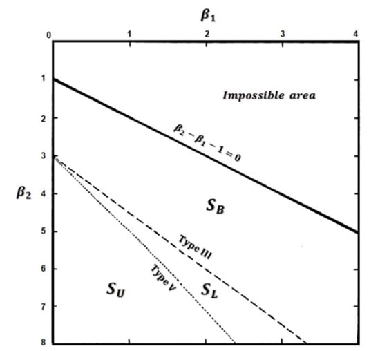
Figure 1. Regions of Johnson’s systems.

Estimates of ${\mathcal{T}}^{*}$ statistic Johnson S_U distribution parameters for different dimensions are given in Table 1.

Table 1. Statistic ${\mathcal{T}}^{*}$ Johnson S_U distribution parameter estimates.

Parameter	Symbol	Estimate
p = 2
Location	$\widehat{\xi }$	4.342807
Scale	$\widehat{\mathsf{\lambda }}$	0.585038
Shape	$\widehat{\delta }$	1.498293
Shape	$\widehat{\gamma }$	0.764906
p = 5
Location	$\widehat{\xi }$	7.025845
Scale	$\widehat{\mathsf{\lambda }}$	0.088023
Shape	$\widehat{\delta }$	0.895003
Shape	$\widehat{\gamma }$	0.400035
p = 10
Location	$\widehat{\xi }$	5.195174
Scale	$\widehat{\mathsf{\lambda }}$	1.578613
Shape	$\widehat{\delta }$	2.24856
Shape	$\widehat{\gamma }$	−1.83037

For statistic ${\mathcal{T}}^{*}$, the invariance and contingency properties were checked. The invariance property is confirmed because standardized data was used. The contingency property is confirmed experimentally (see Section 5).

4. Statistical Distributions

The overviewed normality tests are assessed by the simulation study of 11 statistical distributions grouped into four groups: symmetric, asymmetric, mixed and normal mixture distributions [5]. A description of these distribution groups is given in the following subsections.

4.1. A Group of Symmetric Distributions

Symmetric multivariate distributions are taken from the research [5]:

• Three cases of the Beta(a,b) distribution − Beta(1,1),Beta(1,2) and Beta(2,2), where a and b are the shape parameters.
• One case of the Cauchy(t,s) distribution − Cauchy(0,1), where t and s are the location and scale parameters.
• One case of the Laplace(t,s) distribution − Laplace(0,1), where t and s are the location and scale parameters.
• One case of the Logistic(t,s) distribution − Logistic(0,1), where t and s are the location and scale parameters.
• Two cases of the t-Student(ν) distribution − t(2) and t(5), where ν is the number of degrees of freedom.
• One case of the standard normal N(0,1) distribution.

4.2. A Group of Asymmetric Distributions

Asymmetric multivariate distributions are taken from the research [5]:

• Five cases of the Chi-squared(ν) distribution − χ² (1), χ² (2), χ² (5), χ² (10) and χ² (15), where ν is the number of degrees of freedom.
• Two cases of the Gamma(a,b) distribution − Gamma(0.5,1) and Gamma(5,1), where a and b are the shape and scale parameters.
• One case of the Gumbel(t,s) distribution − Gumbel(1,2), where t and s are the location and scale parameters.
• Two cases of the Lognormal(t,s) distribution − LN(0,1) and LN(0,0.25) where t and s are the location and scale parameters.
• Tree cases of the Weibull(β) distribution − Weibull(0.8), Weibull(1) and Weibull(1.5), where β is the shape parameter.

4.3. A Group of Mixed Distributions

The generated mixed data distribution

$$X_k={\left(X_{k1},X_{k2},\dots ,X_{km},\dots ,X_{kp}\right)}^T, k=1,2,\dots ,n$$

is such that the first m variates (i.e., X_k1, X_k2, …, X_km) follow the standard normal distribution and distribution of the remaining variates is one of the non-normal distributions (Laplace(0,1), χ²(5), t(5), Beta(1,1), Beta(1,2), Beta(2,2)). The experimental research covers the cases for m = p − 1, m = p/2 and m = 1.

4.4. A Group of Normal Mixture Distributions

Normal mixture distributions are considered in this research [5]: nine cases of the multivariate normal mixture distribution MVNMIX (a,b,c,d) − MVNMIX (0.5,2,0,0), MVNMIX (0.5,4,0,0), MVNMIX (0.5,2,0.9,0), MVNMIX (0.5,0.5,0.9,0), MVNMIX (0.5,0.5,0.9,0.1), MVNMIX(0.5,0.5,0.9,0.9), MVNMIX(0.7,2,0.9,0.3), MVNMIX(0.3,1,0.9,0.1), MVNMIX(0.3,1,0.9,0.9). The multivariate normal mixture distribution with density:

$$aN\left(0,{\sum }_1\right)+\left(1-a\right)N\left(b1,{\sum }_2\right),$$

where $1$ is the column vector with all elements being 1,

$${\sum }_1=\left(1-c\right)I+c{11}^T \mathrm{and} {\sum }_2=\left(1-d\right)I+d{11}^T.$$

5. Simulation Study and Discussion

This section provides a modeling study that evaluates the power of selected multivariate normality tests. We used the Monte Carlo method to compare our proposed test with 13 multivariate tests described above for dimensions $p=2, 5, 10$, with sample sizes $n=32, 64, 128, 256, 512, 1024$ at significance level $\alpha =0.05$. Power was estimated by applying the tests on 1 000 000 randomly drawn samples from the alternative distribution (Beta, Cauchy, Laplace, Logistic, Student, Standard normal, Chi-Square, Gamma, Gumbel, Lognormal, Weibull, Mixed, Normal mixture).

The values of the test smoothness parameter ($h$) were selected experimentally: from 0.1 to 5 with a step of 0.1. The value of the test $h$ parameter was determined for each dimension considered. It was found that the best results are obtained (i.e., maximum statistical value) for $p=2$ with $h=1.05$, for $p=5$ with $h=0.1$, and for $p=10$ with $h=2.4$. These smoothness parameter $h$ values were used to carry out the numerical experiments.

The power of 13 (including our proposed test) multivariate goodness of fit hypothesis tests was estimated calculated for different sample sizes, distributions and mixtures. The mean power values for the groups for distributions (given in Section 4), for each test and sample sizes, have been computed and presented in Table 2, Table 3, Table 4 and Table 5. It can be determined that the new test for the groups of symmetric and mixed distributions is the most powerful one. In the group of asymmetric distributions, the new (for $p=2$) and Roy (for $p=5$ and $10$) tests are the most powerful ones. The new (for $p=2$ and $5$) and Roy (for $p=10$ with sample sizes $n=256, 512, 1024$) tests are also the most powerful in the group of normal distribution mixtures. Comparing the Mardia (Mar1 and Mar2) tests, based on asymmetry and excess coefficients, it has been found that Mar1 is the most powerful only for the group of asymmetric distributions. For the group of symmetric distributions the power of this test is the lowest (compared to other tests).

Table 2. An average empirical power for a group of symmetric distributions.

	AD	CHI2	CVM	DH	DN	Energy	HZ	LV	New	Mar1	Mar2	NRR	Roy
p = 2
n = 32	0.651	0.57	0.652	0.677	0.565	0.65	0.644	0.696	0.999	0.532	0.605	0.608	0.703
n = 64	0.778	0.692	0.779	0.809	0.671	0.77	0.765	0.815	0.999	0.617	0.751	0.736	0.819
n = 128	0.867	0.798	0.868	0.892	0.768	0.86	0.853	0.893	0.999	0.681	0.857	0.842	0.891
n = 256	0.92	0.873	0.92	0.932	0.847	0.914	0.906	0.932	0.999	0.721	0.917	0.91	0.929
n = 512	0.939	0.912	0.94	0.945	0.903	0.941	0.936	0.945	0.999	0.743	0.942	0.941	0.944
n = 1024	0.945	0.932	0.945	0.949	0.937	0.948	0.947	0.949	0.999	0.758	0.95	0.949	0.95
p = 5
n = 32	0.644	0.531	0.624	0.735	0.585	0.632	0.622	0.763	0.985	0.523	0.637	0.602	0.784
n = 64	0.791	0.656	0.775	0.864	0.7	0.758	0.755	0.871	0.989	0.621	0.792	0.739	0.875
n = 128	0.883	0.773	0.876	0.924	0.806	0.863	0.856	0.925	0.988	0.696	0.89	0.851	0.924
n = 256	0.929	0.864	0.926	0.941	0.886	0.921	0.91	0.941	0.987	0.735	0.934	0.916	0.941
n = 512	0.942	0.916	0.942	0.946	0.932	0.945	0.94	0.946	0.981	0.752	0.948	0.944	0.947
n = 1024	0.946	0.941	0.946	0.949	0.949	0.949	0.949	0.949	0.985	0.764	0.95	0.95	0.95
p = 10
n = 32	0.557	0.473	0.534	0.754	0.599	0.598	0.604	0.791	0.997	0.458	0.65	0.599	0.834
n = 64	0.754	0.604	0.728	0.884	0.704	0.709	0.71	0.893	0.998	0.592	0.802	0.719	0.905
n = 128	0.878	0.726	0.865	0.934	0.817	0.821	0.831	0.935	0.998	0.676	0.899	0.844	0.934
n = 256	0.928	0.824	0.922	0.941	0.896	0.906	0.901	0.941	0.998	0.733	0.94	0.913	0.943
n = 512	0.942	0.891	0.941	0.945	0.936	0.943	0.937	0.945	0.991	0.747	0.951	0.942	0.946
n = 1024	0.945	0.928	0.945	0.948	0.949	0.948	0.949	0.948	0.991	0.756	0.95	0.949	0.95

Table 3. An average empirical power for a group of asymmetric distributions.

	AD	CHI2	CVM	DH	DN	Energy	HZ	LV	New	Mar1	Mar2	NRR	Roy
p = 2
n = 32	0.634	0.631	0.639	0.852	0.55	0.832	0.811	0.87	0.999	0.813	0.63	0.639	0.877
n = 64	0.744	0.767	0.744	0.956	0.657	0.93	0.906	0.961	0.999	0.941	0.776	0.759	0.962
n = 128	0.827	0.861	0.822	0.995	0.724	0.985	0.968	0.995	0.999	0.992	0.876	0.841	0.995
n = 256	0.897	0.931	0.892	0.999	0.774	0.999	0.995	0.999	0.999	0.999	0.947	0.915	0.999
n = 512	0.954	0.977	0.949	0.999	0.816	0.999	0.999	0.999	0.999	0.999	0.988	0.968	0.999
n = 1024	0.985	0.996	0.982	0.999	0.864	0.999	0.999	0.999	0.999	0.999	0.999	0.993	0.999
p = 5
n = 32	0.614	0.6	0.608	0.915	0.551	0.854	0.798	0.932	0.982	0.803	0.623	0.61	0.945
n = 64	0.763	0.779	0.761	0.99	0.675	0.958	0.907	0.992	0.989	0.954	0.791	0.763	0.993
n = 128	0.869	0.892	0.869	0.999	0.748	0.996	0.974	0.999	0.997	0.997	0.908	0.869	0.999
n = 256	0.946	0.965	0.947	0.999	0.812	0.999	0.998	0.999	0.997	0.999	0.978	0.95	0.999
n = 512	0.984	0.994	0.985	0.999	0.872	0.999	0.999	0.999	0.999	0.999	0.997	0.989	0.999
n = 1024	0.995	0.999	0.995	0.999	0.926	0.999	0.999	0.999	0.999	0.999	0.999	0.999	0.999
p = 10
n = 32	0.483	0.443	0.459	0.944	0.532	0.829	0.744	0.96	0.922	0.693	0.573	0.532	0.98
n = 64	0.707	0.712	0.7	0.998	0.679	0.956	0.861	0.998	0.947	0.931	0.746	0.722	0.999
n = 128	0.863	0.87	0.859	0.999	0.776	0.997	0.954	0.999	0.98	0.997	0.898	0.86	0.999
n = 256	0.955	0.96	0.953	0.999	0.858	0.999	0.994	0.999	0.995	0.999	0.978	0.952	0.999
n = 512	0.99	0.994	0.989	0.999	0.93	0.999	0.999	0.999	0.996	0.999	0.998	0.992	0.999
n = 1024	0.996	0.999	0.996	0.999	0.975	0.999	0.999	0.999	0.996	0.999	0.999	0.999	0.999

Table 4. An average empirical power for a group of mixed distributions.

	AD	CHI2	CVM	DH	DN	Energy	HZ	LV	New	Mar1	Mar2	NRR	Roy
p = 2
n = 32	0.469	0.408	0.463	0.436	0.439	0.582	0.572	0.453	0.999	0.476	0.412	0.444	0.451
n = 64	0.572	0.476	0.567	0.51	0.511	0.703	0.697	0.547	0.999	0.577	0.527	0.533	0.513
n = 128	0.683	0.571	0.679	0.591	0.59	0.809	0.807	0.667	0.999	0.659	0.651	0.641	0.572
n = 256	0.78	0.667	0.778	0.66	0.674	0.872	0.871	0.749	0.999	0.717	0.762	0.741	0.643
n = 512	0.848	0.763	0.847	0.746	0.763	0.895	0.894	0.808	0.999	0.76	0.843	0.827	0.72
n = 1024	0.883	0.842	0.883	0.826	0.835	0.902	0.901	0.857	0.999	0.78	0.884	0.878	0.764
p = 5
n = 32	0.626	0.466	0.585	0.545	0.538	0.703	0.706	0.553	0.982	0.584	0.584	0.551	0.47
n = 64	0.749	0.582	0.726	0.631	0.684	0.788	0.815	0.628	0.989	0.675	0.723	0.694	0.524
n = 128	0.805	0.67	0.791	0.695	0.771	0.845	0.864	0.692	0.995	0.722	0.791	0.769	0.589
n = 256	0.852	0.729	0.841	0.747	0.825	0.88	0.885	0.751	0.998	0.75	0.838	0.822	0.669
n = 512	0.88	0.763	0.875	0.777	0.865	0.894	0.895	0.81	0.999	0.766	0.864	0.863	0.73
n = 1024	0.894	0.789	0.893	0.795	0.891	0.9	0.899	0.883	0.999	0.778	0.889	0.889	0.764
p = 10
n = 32	0.688	0.477	0.642	0.58	0.669	0.719	0.745	0.592	0.916	0.614	0.731	0.679	0.475
n = 64	0.753	0.579	0.744	0.69	0.753	0.744	0.78	0.69	0.942	0.68	0.796	0.753	0.529
n = 128	0.775	0.651	0.771	0.736	0.776	0.777	0.821	0.735	0.94	0.722	0.795	0.774	0.602
n = 256	0.802	0.709	0.795	0.761	0.793	0.823	0.87	0.76	0.968	0.745	0.811	0.79	0.689
n = 512	0.833	0.746	0.821	0.778	0.818	0.875	0.892	0.776	0.995	0.764	0.84	0.814	0.745
n = 1024	0.866	0.763	0.853	0.791	0.842	0.897	0.899	0.79	0.997	0.779	0.861	0.837	0.769

Table 5. An average empirical power for a group of normal mixture distributions.

	AD	CHI2	CVM	DH	DN	Energy	HZ	LV	New	Mar1	Mar2	NRR	Roy
p = 2
n = 32	0.465	0.422	0.468	0.56	0.428	0.537	0.529	0.588	0.999	0.433	0.437	0.442	0.607
n = 64	0.576	0.508	0.581	0.74	0.503	0.682	0.672	0.752	0.999	0.544	0.563	0.544	0.778
n = 128	0.71	0.618	0.715	0.893	0.582	0.836	0.823	0.895	0.999	0.633	0.707	0.664	0.908
n = 256	0.844	0.738	0.848	0.974	0.685	0.938	0.926	0.974	0.999	0.701	0.84	0.805	0.978
n = 512	0.943	0.845	0.945	0.998	0.791	0.986	0.977	0.998	0.999	0.733	0.931	0.924	0.998
n = 1024	0.987	0.917	0.988	0.999	0.882	0.999	0.998	0.999	0.999	0.757	0.977	0.985	0.999
p = 5
n = 32	0.45	0.399	0.441	0.594	0.443	0.503	0.485	0.632	0.98	0.384	0.46	0.442	0.672
n = 64	0.574	0.491	0.563	0.782	0.51	0.64	0.621	0.795	0.994	0.516	0.59	0.539	0.828
n = 128	0.699	0.598	0.689	0.916	0.594	0.781	0.761	0.92	0.997	0.619	0.728	0.655	0.934
n = 256	0.806	0.702	0.798	0.979	0.691	0.894	0.877	0.979	0.999	0.694	0.832	0.766	0.984
n = 512	0.889	0.787	0.883	0.998	0.782	0.963	0.95	0.998	0.999	0.736	0.905	0.857	0.998
n = 1024	0.946	0.857	0.942	0.999	0.859	0.992	0.985	0.999	0.999	0.758	0.954	0.925	0.999
p = 10
n = 32	0.402	0.392	0.396	0.62	0.495	0.476	0.487	0.667	0.989	0.287	0.547	0.487	0.735
n = 64	0.556	0.47	0.537	0.8	0.536	0.599	0.581	0.815	0.984	0.472	0.634	0.55	0.855
n = 128	0.709	0.587	0.692	0.915	0.629	0.723	0.708	0.919	0.977	0.582	0.758	0.674	0.939
n = 256	0.801	0.688	0.79	0.973	0.723	0.834	0.815	0.974	0.971	0.669	0.834	0.771	0.98
n = 512	0.853	0.76	0.846	0.995	0.8	0.912	0.887	0.995	0.971	0.711	0.885	0.833	0.997
n = 1024	0.893	0.818	0.886	0.999	0.85	0.96	0.939	0.999	0.973	0.739	0.924	0.875	0.999

In order to supplement and emphasize the results presented in Table 2, Table 3, Table 4 and Table 5, the generalized line diagrams were drawn using the Trellis display [26] multivariate data visualization method. The resulting graph is shown in Figure 2 which shows that the New test is significantly more powerful than the other tests. The power of the Mar1 tests is the lowest compared with the other tests. Figure 2 indicate that the power of the tests increases as the sample size increases. By increasing the dimensions of the power of 8 (AD, CHI2, CVM, Energy, HZ, New, Mar1 and NRR) tests decreases while the power of the other (DH, DN, LV, Mar2 and Roy) tests increases slightly. For small sample sizes, the most powerful tests are New, Roy and DH. For large sample sizes, the most powerful tests are New, Energy, HZ and LV.

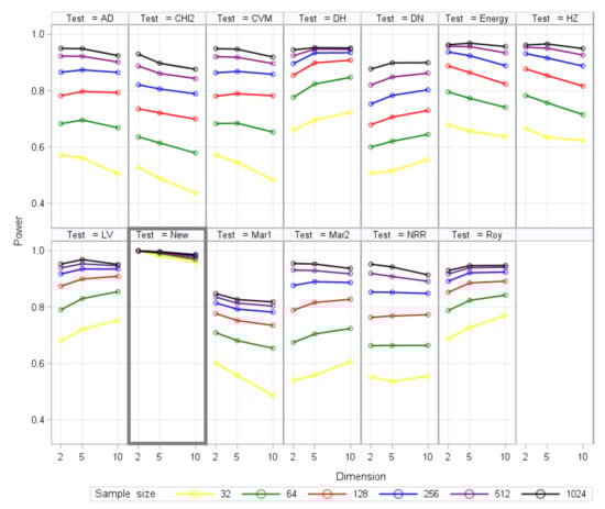
Figure 2. The summary of average empirical power of all examined distribution groups by sample size and dimensionality.

6. Examples

6.1. Survival Data

The data set collected in 2001–2020 by the Head of the Department of Urology Clinic of the Lithuanian University of Health Sciences [27] illustrates the practical application. This dataset consists of study data from 2423 patients and two different continuous attributes (patient age and prostate-specific antigen (PSA)). The assumption of normality was verified by filtering patients’ age and PSA by year of death (i.e., deaths during the first 1, 2, 3, 4, 5, 6, 7, 10, and 15 years). The filtered data was standardized. The power and p-value were calculated for the multivariate tests. The significance level of $\alpha =0.05$ was used for the study. Based on the obtained results, it was found that all the applied multivariate tests rejected the $H_0$ the hypothesis of normality. The power of tests CHI2, DH, Energy, HZ, LV, New, Mar, NRR and Roy was 0.999 and the p-value was <0.0001. Except for DN test, which power was 0.576 and the p-value was 0.026.

6.2. IQOS Data

In 2017, the data set of pollution research with IQOS and traditional cigarettes [28] was used by Kaunas University of Technology, Faculty of Chemical Technology, and Department of Environmental Technology for practical application. This data set consists of 33 experiments (with different conditions) in which the numerical (Pn10) and mass concentrations (Pm2.5, Pm10) of particles were measured. The assumption of normality was checked by filtering Pn10, Pm2.5, Pm10 according to the number of the experiment in the smoking phase. The filtered data was standardized. The power and p-values of multivariate tests with a significance level of $\alpha =0.05$ were calculated. Based on the obtained results, it was found that all the applied multivariate tests show that the assumption of normality is rejected. Most of the multivariate tests used (CHI2, DH, Energy, HZ, LV, New, Mar, NRR, and Roy) had a power of 0.999 and p-value of <0.0001. The power of the other tests was also close to 0.99 and the p-value was about 0.0001.

7. Conclusions

In this study, the comprehensive comparison of the power of 13 multivariate goodness of fit tests was performed for groups of symmetric, asymmetric, mixed, and normal mixture distributions. Two-dimensional, five-dimensional, and ten-dimensional data sets were generated to estimate the test power empirically.

A new multivariate goodness of fit test based on inversion formula was proposed. Based on the obtained modeling results, it was determined that the most powerful tests for the groups of symmetric, asymmetric mixed and normal mixture distributions are the proposed test and Roy multivariate test. From two real data examples, it was concluded that our proposed test is stable, even when applied to real data sets.

References

- Henze, N.; Zirkler, B. A class of invariant consistent tests for multivariate normality. Commun. Stat. Theory Methods 1990, 19, 3595–3617. [Google Scholar] [CrossRef]
- Henze, N. Invariant tests for multivariate normality: A critical review. Stat. Pap. 2002, 43, 467–506. [Google Scholar] [CrossRef]
- Royston, J.P. An extension of Shapiro and Wilk’s W test for normality to large samples. Appl. Stat. 1982, 31, 115–124. [Google Scholar] [CrossRef]
- Ross, G.J.S.; Hawkins, D. MLP: Maximum Likelihood Program; Rothamsted Experimental Station: Harpenden, UK, 1980. [Google Scholar]
- Korkmaz, S.; Goksuluk, D.; Zararsiz, G. MVN: An R Package for Assessing Multivariate Normality. R J. 2014, 6, 151–162. [Google Scholar] [CrossRef]
- Doornik, J.A.; Hansen, H. An Omnibus Test for Univariate and Multivariate Normality. Oxf. Bull. Econ. Stat. 2008, 70, 927–939. [Google Scholar]
- Voinov, V.; Pya, N.; Makarov, R.; Voinov, Y. New invariant and consistent chi-squared type goodness-of-fit tests for multivariate normality and a related comparative simulation study. Commun. Stat. Theory Methods 2016, 45, 3249–3263. [Google Scholar] [CrossRef]
- Moore, D.S.; Stubblebine, J.B. Chi-square tests for multivariate normality with application to common stock prices. Commun. Stat. Theory Methods 1981, A10, 713–738. [Google Scholar] [CrossRef]
- Gnanadesikan, R.; Kettenring, J.R. Robust estimates, residuals, and outlier detection with multiresponse data. Biometrics 1972, 28, 81–124. [Google Scholar]
- Górecki, T.; Horváth, L.; Kokoszka, P. Tests of Normality of Functional Data. Int. Stat. Rev. 2020, 88, 677–697. [Google Scholar] [CrossRef]
- Pinto, L.P.; Mingoti, S.A. On hypothesis tests for covariance matrices under multivariate normality. Pesqui. Operacional. 2015, 35, 123–142. [Google Scholar] [CrossRef][Green Version]
- Dörr, P.; Ebner, B.; Henze, N. A new test of multivariate normality by a double estimation in a characterizing PDE. Metrika 2021, 84, 401–427. [Google Scholar] [CrossRef]
- Zhoua, M.; Shao, Y. A Powerful Test for Multivariate Normality. J. Appl Stat. 2014, 41, 351–363. [Google Scholar] [CrossRef]
- Kolkiewicz, A.; Rice, G.; Xie, Y. Projection pursuit based tests of normality with functional data. J. Stat. Plan. Inference 2021, 211, 326–339. [Google Scholar] [CrossRef]
- Ebner, B.; Henze, N. Tests for multivariate normality-a critical review with emphasis on weighted L^2-statistics. TEST 2020, 29, 845–892. [Google Scholar] [CrossRef]
- Arnastauskaitė, J.; Ruzgas, T.; Bražėnas, M. An Exhaustive Power Comparison of Normality Tests. Mathematics 2021, 9, 788. [Google Scholar] [CrossRef]
- Mardia, K. Measures of Multivariate Skewness and Kurtosis with Applications. Biometrika 1970, 57, 519–530. [Google Scholar] [CrossRef]
- Szekely, J.G.; Rizzo, L.M. Energy statistics: A class of statistics based on distances. J. Stat. Plan. Inference 2013, 143, 1249–1272. [Google Scholar] [CrossRef]
- Lobato, I.; Velasco, C. A simple Test of Normality for Time Series. Econom. Theory 2004, 20, 671–689. [Google Scholar] [CrossRef]
- Ruzgas, T. The Nonparametric Estimation of Multivariate Distribution Density Applying Clustering Procedures. Ph.D. Thesis, Institute of Mathematics and Informatics, Vilnius, Lithuania, 2007; p. 161. [Google Scholar]
- Marron, J.S.; Wand, M.P. Exact mMean Integrated Squared Error. Ann. Stat. 1992, 20, 712–736. [Google Scholar] [CrossRef]
- Kavaliauskas, M.; Rudzkis, R.; Ruzgas, T. The Projection-based Multivariate Distribution Density Estimation. Acta Comment. Univ. Tartu. Math. 2004, 8, 135–141. [Google Scholar]
- Epps, T.W.; Pulley, L.B. A test for normality based on the empirical characteristic function. Biometrika 1983, 70, 723–726. [Google Scholar] [CrossRef]
- Johnson, N.L. Systems of Frequency Curves Generated by Methods of Translation. Biometrika 1949, 36, 149–176. [Google Scholar] [CrossRef] [PubMed]
- Wicksell, S.D. The construction of the curves of equal frequency in case of type A correlation. Ark. Mat. Astr. Fys. 1917, 12, 1–19. [Google Scholar]
- Theus, M. High Dimensional Data Visualization. In Handbook of Data Visualization; Springer: Berlin/Heidelberg, Germany, 2008; pp. 5–7. [Google Scholar]
- Milonas, D.; Ruzgas, T.; Venclovas, Z.; Jievaltas, M.; Joniau, S. The significance of prostate specific antigen persistence in prostate cancer risk groups on long-term oncological outcomes. Cancers 2021, 13, 2453. [Google Scholar] [CrossRef]
- Martuzevicius, D.; Prasauskas, T.; Setyan, A.; O’Connell, G.; Cahours, X.; Julien, R.; Colard, S. Characterization of the Spatial and Temporal Dispersion Differences Between Exhaled E-Cigarette Mist and Cigarette Smoke. Nicotine Tob. Res. 2019, 21, 1371–1377. [Google Scholar] [CrossRef]
Publisher’s Note: MDPI stays neutral with regard to jurisdictional claims in published maps and institutional affiliations. |
© 2021 by the authors. Licensee MDPI, Basel, Switzerland. This article is an open access article distributed under the terms and conditions of the Creative Commons Attribution (CC BY) license (https://creativecommons.org/licenses/by/4.0/).