A Reverse Non-Stationary Generalized B-Splines Subdivision Scheme

Abstract

In this paper, two new families of non-stationary subdivision schemes are introduced. The schemes are constructed from uniform generalized B-splines with multiple knots of orders 3 and 4, respectively. Then, we construct a third-order reverse subdivision framework. For that, we derive a generalized multi-resolution mask based on their third-order subdivision filters. For the reverse of the fourth-order scheme, two methods are used; the first one is based on least-squares formulation and the second one is based on solving a linear optimization problem. Numerical examples are given to show the performance of the new schemes in reproducing different shapes of initial control polygons.

1. Introduction

In recent years, the usage of subdivision schemes played a crucial role in developing computer graphics and creating smooth curves and surfaces. The starting point of this theory was Rahm’s article (see [1]); a few years later several schemes were developed to extend the field of application to more complicated curves and surfaces. This theory has found huge success in many fields of application such as curve and surface reconstruction (see [2,3,4,5]), computer animation and graphics (see [6,7,8]), robotics (see [9]), medical science processing (see [10,11,12]), wavelet and frame construction (see [13,14,15,16]), etc. Subdivision schemes have a very strong link with splines, so they are widely used to describe various properties of splines such as shape reproduction and approximation order calculation [17,18,19]. In the numerical domain, different subdivision schemes to approximate numerically various curves and surfaces have been proposed. For example, in [20] Romani has presented non-stationary approximating subdivision schemes to reproduce exponential functions based on algebraic and exponential polynomials. In Sunita and Shunmugaraj [4], an interpolating non-stationary subdivision schemes was introduced to generate circles, ellipses and all functions spanned by $\{1,cos(x),sin(x\left)\right\}$. Recent proposals of efficient non-stationary subdivision schemes have been presented by Ghaffar et al. [21], Fakhar et al. [22,23], Siddiqi et al. [24,25], where the authors have built elegant methods capable of reproducing complex curves or surfaces.

The reverse subdivision is a very important topic in CAGD that is often used in the removal of noise from curves and surfaces. For example, In [26], Foster et al. gave an idea of how the reverse subdivision can be used to remove and filter artifacts and noises from silhouettes extracted from polygonal meshes. To reduce the number of vertices in the raw data of a digitized leaf, Mundermann et al. [27] used the same idea as Foster et al. [26].

However, few works discuss the construction of wavelets based on the reverse subdivision technique. For example, Samavati and Bartels [15] are the first researchers who used the notion of reverse subdivision method for constructing multiresolution representation and studied its application to derive local reverse subdivision filters using local linear conditions (see [16]). Reference [28], Sadeghi et al. developed a full multiresolution representation based on reverse subdivision to create a good and smooth approximation of the original control points. In [29], Mohamed F. Hassan and Neil A. Dodgson presented a reverse Chaikin algorithm that generates a multiresolution representation of any line chain. For the non-interpolating transforms construction relies on the recently-introduced decimation operators, see [30] which are employed as subsampling operators. Recently, M. Ajeddar and A. Lamnii (see [31]) construct the inverse subdivision scheme associated with the quadratic uniform algebraic hyperbolic (UAH) B-spline by following the method introduced in [29].

In this paper, we introduce generalized B-splines of order 3 and 4 with multiple knots. From these B-splines, we have constructed two non-stationary subdivision schemes called generalized subdivision schemes of order 3 and 4. These subdivision schemes can exactly reproduce trigonometric and hyperbolic limit curves. As the matrix corresponding to the generalized subdivision scheme of order 3 is a square matrix, we compute the inverse of this matrix to finally obtain the expression of the reverse scheme of order 3. Using the multiresolution theory we propose the wavelets corresponding to the generalized scheme of order 3. To calculate the reverse generalized scheme of order 4 we use two methods: the first is similar to the one presented by Olsen in [32] which is based on multiresolution. It starts by finding the approximate reverse scheme and then finding the error between the control polygonal and the one constructed by using this approximate reverse scheme. The calculation of this error is based on the solution of least-squares formulations. Precisely the second method differs from the first one in this part of the error calculation. It is based on the matrix solution of a linear optimization problem such that the error is minimized. The great advantage of this method is that the error depends on the generalized subdivision of order 4 matrix which is already known. The corresponding algorithm is also presented.

The main novelty of this paper is that our reverse subdivision scheme is a non-stationary reverse scheme that is characterized by a tension parameter that allows us to exactly reproduce the initial control polygonal of the trigonometric and hyperbolic form. The performance of the proposed schemes compared to those in the literature is illustrated by numerical examples.

The paper is organized as follows. We first introduce the definition and some interesting properties of the generalized B-splines of degree 3 and 4 of the proposed subdivision scheme in Section 2. In Section 3, we present the subdivision scheme associated with the generalized B-spline. Section 4, presents the reverse subdivision scheme for generalized B-splines of degree 3. Moreover, a related multiresolution technique is discussed. In Section 5, based on two methods, we give the reverse subdivision scheme for generalized B-splines of degree 4. The last section is devoted to the conclusion.

2. Definitions of Generalized B-Spline Basis Functions

This section aims to present explicit formulas of the uniform generalized B-splines of order k where $k\in \left\{3,4\right\}$ and gave their interesting properties, for more details see [5,33]. To do this, we need the following notations:

For a given positive integer $\ell >0$, let $h_{\ell }=\frac{b-a}{2^{\ell }}$ and $\omega \in {\mathbb{R}}_{+}\cup i{\mathbb{R}}_{+}$ such that $0<\left|w\right|h<\pi .$ Let,

$$\begin{array}{cc}\hfill {\tau }_{\ell }& =\{t_{-k}=\cdots =t_0,t_1,\cdots ,t_{2^{\ell }-1},t_{2^{\ell }}=\cdots =t_{2^{\ell }+k}\}\hfill \\ \hfill & =\{\underset{(k+1)\mathrm{equal}\mathrm{knots}}{\underbrace{a,\dots ,a}},\underset{(2^{\ell }-1)\mathrm{internal}\mathrm{knots}}{\underbrace{a+h_{\ell },\cdots ,a+(2^{\ell }-1)h_{\ell }}},\underset{(k+1)\mathrm{equal}\mathrm{knots}}{\underbrace{b,\dots ,b}}\}\hfill \end{array}$$

the uniform partition of $I=[a,b]$, with meshlength $h_{\ell }$ and $S_k\left(I,{\tau }_{{}^{\ell }}\right)$ the space of generalized splines of order k defined by:

$$S_k\left(I,{\tau }_{{}^{\ell }}\right)=\left\{s\in {\mathcal{C}}^{k-2}\left([a,b]\right),s_{{\mid }_{[t_i,t_{i+1}]}}\in {\mathsf{\Gamma }}_k\right\}$$

where ${\mathsf{\Gamma }}_k=span\{1,t^{k-3},cos\left(\omega t\right),sin\left(\omega t\right)\}.$

The dimension of $S_k\left(I,{\tau }_{\ell }\right)$ is $(2^{\ell }+k-1)$ and the k-order generalized B-splines are given by:

• For $k=3$:

  $$\begin{array}{cc}\hfill N_{1,3}\left(t\right)& :=\left\{\begin{array}{cc}\frac{cos\left(\omega (t_1-x)\right)-1}{cos\left(h_{\ell }\omega \right)-1},\hfill & t\in [t_0,t_1]\hfill \\ 0,\hfill & \mathrm{otherwise}\hfill \end{array}\right.\hfill \\ \hfill N_{2,3}\left(t\right)& :=\left\{\begin{array}{cc}\frac{-2cos\left(\omega (t_1-t)\right)+2cos\left(h_{\ell }\omega \right)-cos\left(\omega t\right)+1}{2cos\left(h_{\ell }\omega \right)-2},\hfill & t\in [t_0,t_1]\hfill \\ \frac{1}{2}{csc}^2\left(\frac{h_{\ell }\omega }{2}\right){sin}^2\left(\omega (t_1-\frac{t}{2})\right),\hfill & t\in [t_1,t_2]\hfill \\ 0,\hfill & \mathrm{otherwise}\hfill \end{array}\right.\hfill \\ \hfill N_{2^{\ell }+1,3}\left(t\right)& :=\left\{\begin{array}{cc}-\frac{cos(\omega (t-t_{m_{\ell }-2})-1)}{2(cosh(\omega h)-1)},\hfill & t\in [t_{2^{\ell }-2},t_{2^{\ell }-1}]\hfill \\ \frac{-cos\left(\omega (t_{\ell }-t)\right)-2cos\left(\omega (t-t_{2^{\ell }-1})\right)+2cos\left(h_{\ell }\omega \right)+1}{2cos\left(h_{\ell }\omega \right)-2},\hfill & t\in [t_{2^{\ell }-1},t_{2^{\ell }}]\hfill \\ 0,\hfill & \mathrm{otherwise}\hfill \end{array}\right.\hfill \\ \hfill N_{2^{\ell }+2,3}\left(t\right)& :=\left\{\begin{array}{cc}\frac{cos\left(\omega (t-t_{2^{\ell }-1})\right)-1}{cos\left(h_{\ell }\omega \right)-1},\hfill & t\in [t_{2^{\ell }-1},t_{2^{\ell }}]\hfill \\ 0,\hfill & \mathrm{otherwise}\hfill \end{array}\right.\hfill \end{array}$$

  and

  $$N_{i,3}\left(t\right):=N_3\left(t-t_{i-2}\right),3\le i\le 2^{\ell }$$

  where

  $$N_3\left(t\right):=\left\{\begin{array}{cc}\frac{cos\left(w(t-t_0)\right)-1}{2(cos\left(h_{\ell }w\right)-1)},\hfill & t\in [t_0,t_1]\hfill \\ \frac{-cos\left(w(t_2-x)\right)-cos\left(w(x-t_1)\right)+2cos\left(h_{\ell }w\right)}{2(cos\left(h_{\ell }w\right)-1)},\hfill & t\in [t_1,t_2]\hfill \\ \frac{cos\left(w(t_3-t)\right)-1}{2(cos\left(h_{\ell }w\right)-1)},\hfill & t\in [t_2,t_3]\hfill \\ 0,\hfill & \mathrm{otherwise}\hfill \end{array}\right.$$
• For $k=4$:

  $$\begin{array}{cc}\hfill N_{1,4}\left(t\right)& :=\left\{\begin{array}{cc}\frac{\omega (t-t_1)+sin\left(\omega (t_1-t)\right)}{sin\left(h_{\ell }\omega \right)-h_{\ell }\omega },\hfill & t\in [t_0,t_1]\hfill \\ 0,\hfill & \mathrm{otherwise}\hfill \end{array}\right.\hfill \\ \hfill N_{2^{\ell }+3,4}\left(t\right)& :=\left\{\begin{array}{cc}\frac{sin\left(\omega (t-t_{2^{\ell }-1})\right)+\omega (-t+t_{2^{\ell }-1})}{sin\left(h_{\ell }\omega \right)-h_{\ell }\omega },\hfill & t\in [t_{2^{\ell }-1},t_{2^{\ell }}]\hfill \\ 0,\hfill & \mathrm{otherwise}\hfill \end{array}\right.\hfill \\ \hfill N_{2,4}\left(t\right)& :=\left\{\begin{array}{c}\frac{sin\left(\omega (t_1-t)\right)-sin\left(h_{\ell }\omega \right)+\omega (t-t_0)}{h_{\ell }\omega -sin\left(h_{\ell }\omega \right)}+\hfill \\ \frac{-2sin\left(\omega (t_1-t)\right)-2\omega (t-t_0)cos\left(h_{\ell }\omega \right)+2sin\left(h_{\ell }\omega \right)-\omega (t-t_0)+sin\left(\omega (t-t_0)\right)}{2h_{\ell }\omega cos\left(h_{\ell }\omega \right)-2sin\left(h_{\ell }\omega \right)},\hfill & t\in [t_0,t_1]\hfill \\ \frac{\omega (t-t_2)+sin\left(\omega (t_2-t)\right)}{2h_{\ell }\omega cos\left(h_{\ell }\omega \right)-2sin\left(h_{\ell }\omega \right)},\hfill & t\in [t_1,t_2]\hfill \\ 0,\hfill & \mathrm{otherwise}.\hfill \end{array}\right.\hfill \\ \hfill N_{2^{\ell }+2,4}\left(t\right)& :=\left\{\begin{array}{cc}\frac{sin(\omega (t-t_{2^{\ell }-2})+\omega (t_{2^{\ell }-2}-t)}{2h_{\ell }\omega cos\left(h_{\ell }\omega \right)-2sin\left(h_{\ell }\omega \right)},\hfill & t\in [t_{2^{\ell }-2},t_{2^{\ell }-1}]\hfill \\ -\frac{\omega ((t_{2^{\ell }-1}-t)sin\left(2h_{\ell }\omega \right)+h_{\ell }(-2sin\left(\omega (t-t_{2^{\ell }-1})\right)+sin\left(\omega (t-t_{2^{\ell }-2})\right)}{2(sin\left(h_{\ell }\omega \right)-h_{\ell }\omega w)(h_{\ell }\omega cos\left(h_{\ell }\omega \right)-sin\left(h_{\ell }\omega \right))}\hfill \\ -\frac{\omega (t-t_{2^{\ell }})-sin\left(h_{\ell }\omega \right)(sin\left(\omega (t_{2^{\ell }}-t)\right)+\omega (t_{2^{\ell }-2}-t)}{2(sin\left(h_{\ell }\omega \right)-h_{\ell }\omega w)(h_{\ell }\omega cos\left(h_{\ell }\omega \right)-sin\left(h_{\ell }\omega \right))},\hfill & t\in [t_{2^{\ell }-1},t_{2^{\ell }}]\hfill \\ 0,\hfill & \mathrm{otherwise}.\hfill \end{array}\right.\hfill \\ \hfill N_{3,4}\left(t\right)& :=\left\{\begin{array}{c}\frac{\omega (t-t_0)-sin\left(\omega (t-t_0)\right)}{2h_{\ell }\omega cos\left(h_{\ell }\omega \right)-2h_{\ell }\omega }+\hfill \\ \frac{2sin\left(\omega (t_1-t)\right)+2\omega (t-t_0)cos\left(h_{\ell }\omega \right)-2sin\left(h_{\ell }\omega \right)+\omega (t-t_0)-sin\left(\omega (t-t_0)\right)}{2h_{\ell }\omega cos\left(h_{\ell }\omega \right)-2sin\left(h_{\ell }\omega \right)},\hfill & t\in [t_0,t_1]\hfill \\ \frac{2h_{\ell }{\omega }^2(t_2-t){cos}^2\left(h_{\ell }\omega \right)-\omega (t_2-t)(h_{\ell }\omega +sin\left(2h_{\ell }\omega \right))+h_{\ell }\omega sin\left(\omega (t_2-t)\right)+sin\left(h_{\ell }\omega \right)(sin\left(\omega (t_1-t)\right)}{2h_{\ell }\omega (cos\left(h_{\ell }\omega \right)-1)(h_{\ell }\omega cos\left(h_{\ell }\omega \right)-sin\left(h_{\ell }\omega \right))}+\hfill \\ \frac{sin\left(\omega (t_2-t)\right)+h_{\ell }\omega )-h_{\ell }\omega cos\left(h_{\ell }\omega \right)(sin\left(\omega (t_1-t)\right)+2sin\left(\omega (t_2-t)\right)+\omega (t-t_1))}{2h_{\ell }\omega (cos\left(h_{\ell }\omega \right)-1)(h_{\ell }\omega cos\left(h_{\ell }\omega \right)-sin\left(h_{\ell }\omega \right))},\hfill & t\in [t_1,t_2]\hfill \\ \frac{sin\left(\omega (t_3-t)\right)+\omega (t-t_3)}{2h_{\ell }\omega cos\left(h_{\ell }\omega \right)-2h_{\ell }w}\hfill & t\in [t_2,t_3]\hfill \\ 0,\hfill & \mathrm{otherwise}.\hfill \end{array}\right.\hfill \end{array}$$

  $$\begin{array}{cc}\hfill N_{2^{\ell }+1,4}\left(t\right)& :=\left\{\begin{array}{cc}-\frac{\omega (t-t_{2^{\ell }-3})+sin\left(\omega (t_{2^{\ell }-3}-t)\right)}{2h_{\ell }\omega (cos\left(h_{\ell }\omega \right)-1)},\hfill & t\in [t_{2^{\ell }-3},t_{2^{\ell }-2}]\hfill \\ \frac{\omega (t-t_{2^{\ell }-2})+sin\left(\omega (t_{2^{\ell }-2}-t)\right)}{2h_{\ell }\omega cos\left(h_{\ell }\omega \right)-2sin\left(h_{\ell }\omega \right)}+\frac{sin\left(h_{\ell }\omega \right)-h_{\ell }\omega }{2h_{\ell }\omega cos\left(h_{\ell }\omega \right)-2h_{\ell }\omega }\hfill \\ \frac{sin\left(\omega (t-t_{2^{\ell }-1})\right)+sin\left(\omega (t-t_{2^{\ell }-2})\right)+2\omega (t_{2^{\ell }-2}-t)cos\left(h_{\ell }\omega \right)+sin\left(h_{\ell }\omega \right)}{2h_{\ell }\omega (cos\left(h_{\ell }\omega \right)-1)},\hfill & t\in [t_{2^{\ell }-2},t_{2^{\ell }-1}]\hfill \\ \frac{h_{\ell }{\omega }^2(t_{2^{\ell }}-t)cos\left(2h_{\ell }\omega \right)-h_{\ell }\omega (sin\left(\omega (t_{2^{\ell }-1}-t)\right)+sin\left(\omega (t-t_{2^{\ell }-1})\right)-sin\left(\omega (t-t_{2^{\ell }-2})\right)}{2h_{\ell }\omega (cos\left(h_{\ell }\omega \right)-1)(h_{\ell }\omega cos\left(h_{\ell }\omega \right)-sin\left(h_{\ell }\omega \right))}+\hfill \\ \frac{sin\left(2h_{\ell }\omega \right))+sin\left(h_{\ell }\omega \right)(\omega (t-t_{2^{\ell }-2})+sin\left(\omega (t_{2^{\ell }}-t)\right))}{2h_{\ell }\omega (cos\left(h_{\ell }\omega \right)-1)(h_{\ell }\omega cos\left(h_{\ell }\omega \right)-sin\left(h_{\ell }\omega \right))},\hfill & t\in [t_{2^{\ell }-1},t_{2^{\ell }}]\hfill \\ 0,\hfill & \mathrm{otherwise}.\hfill \end{array}\right.\hfill \end{array}$$

  and

  $$N_{i,4}\left(t\right):=N_4\left(t-t_{i-2}\right),4\le i\le 2^{\ell }$$

  where

  $$N_4\left(t\right)=\left\{\begin{array}{cc}\frac{sin\left(\omega (t-t_0)\right)-\omega (t-t_0)}{2h_{\ell }\omega cos\left(h_{\ell }\omega \right)-2h_{\ell }\omega },\hfill & t\in [t_0,t_1]\hfill \\ \frac{2sin\left(\omega (t_1-t)\right)+sin\left(\omega (t_2-t)\right)+2\omega (t-t_1)cos\left(h_{\ell }\omega \right)+\omega (t-t_2)}{2h_{\ell }\omega (cos\left(h_{\ell }\omega \right)-1)},\hfill & t\in [t_1,t_2]\hfill \\ \frac{-sin\left(\omega (t_2-t)\right)-2sin\left(\omega (t_3-t)\right)-2\omega (t-t_0)cos\left(h_{\ell }\omega \right)+2h_{\ell }\omega +6h_{\ell }\omega cos\left(h_{\ell }\omega \right)-\omega x}{2h_{\ell }\omega (cos\left(h_{\ell }\omega \right)-1)},\hfill & t\in [t_2,t_3]\hfill \\ \frac{sin\left(\omega (t_4-t)\right)+\omega (t-t_4)}{2h_{\ell }\omega cos\left(h_{\ell }\omega \right)-2h_{\ell }\omega },\hfill & t\in [t_3,t_4]\hfill \\ 0,\hfill & \mathrm{otherwise}\hfill \end{array}\right.$$

In [5], M.-E. Fang et al. proved that all the desirable properties of classical polynomial B-splines carry over to the generalized B-splines of order k. In this section, we mention only the most remarkable ones such as:

• Local support: $N_{i,k}\left(t\right)=0$ for $t\notin [t_i,t_{i+k}]$.
• Positivity: $N_{i,k}\left(t\right)>0$ for $\left.t\in \right]t_i,t_{i+k}[$.
• Partition of unity: ${\displaystyle \sum _{i=1}^{2^{\ell }+k-1}{N}_{i,k}\left(t\right)=1,}$ for all $t\in [a,b].$
• Linear independence: $N_{1,k},\cdots ,N_{2^{\ell }+k-1,k}$ are linearly independent.

3. Generalized Subdivision Scheme

This section presents the explicit matrix form of the generalized subdivision scheme corresponding to the B-spline proposed in the previous Section, afterwards illustrating some numerical examples of the application of this scheme in generating limit curves.

3.1. Generalized Subdivision Rules

By using the same method described in [5], we can also propose a generalized subdivision scheme from the refinement equation associated with the generalized B-spline with multiple knots of order k.

Let $C^0={\left\{c_{-2}^0,\dots ,c_n^0\right\}}^T$ be the vector of initial data and $u^0$ be a tension parameter satisfying $u^0>0$. The generalized subdivision scheme of order k at level ℓ can be written in matrix form:

$$C^{\ell +1}=P_k^{\ell }{C}^{\ell },\ell \ge 0.$$

(1)

where $P_k^{\ell }$ is the matrix of the generalized subdivision scheme of order k at level ℓ, its expression for $k=3$ is   

$$P_3^{\ell }=\left(\begin{array}{cccccccc}1& 0& 0& 0& \cdots & 0& 0& 0\\ \frac{1}{1+u^{\ell }}& \frac{u^{\ell }}{1+u^{\ell }}& 0& 0& \cdots & 0& 0& 0\\ 0& \frac{1+2u^{\ell }}{2(1+u^{\ell })}& \frac{1}{2(1+u^{\ell })}& 0& \cdots & 0& 0& 0\\ 0& \frac{1}{2(1+u^{\ell })}& \frac{1+2u^{\ell }}{2(1+u^{\ell })}& 0& \cdots & 0& 0& 0\\ 0& 0& \frac{1+2u^{\ell }}{2(1+u^{\ell })}& \frac{1}{2(1+u^{\ell })}& \cdots & 0& 0& 0\\ 0& 0& \frac{1}{2(1+u^{\ell })}& \frac{1+2u^{\ell }}{2(1+u^{\ell })}& \cdots & 0& 0& 0\\ ⋮& ⋮& ⋮& ⋮& \ddots & ⋮& ⋮& ⋮\\ 0& 0& 0& 0& \cdots & \frac{1+2u^{\ell }}{2(1+u^{\ell })}& \frac{1}{2(1+u^{\ell })}& 0\\ 0& 0& 0& 0& \cdots & \frac{1}{2(1+u^{\ell })}& \frac{1+2u^{\ell }}{2(1+u^{\ell })}& 0\\ 0& 0& 0& 0& \cdots & 0& \frac{u^{\ell }}{1+u^{\ell }}& \frac{1}{1+u^{\ell }}\\ 0& 0& 0& 0& \cdots & 0& \cdots & 1\end{array}\right),$$

(2)

and for $k=4$ it is

$$P_4^{\ell }=\left(\begin{array}{ccccccccc}1& 0& 0& 0& 0& \cdots & 0& 0& 0\\ \frac{1}{1+u^{\ell }}& \frac{u^{\ell }}{1+u^{\ell }}& 0& 0& 0& \cdots & 0& 0& 0\\ 0& \frac{1+2u^{\ell }}{2(1+u^{\ell })}& \frac{1}{2(1+u^{\ell })}& 0& 0& \cdots & 0& 0& 0\\ 0& \frac{1+2u^{\ell }}{8(1+u^{\ell })}& \frac{5+6u^{\ell }}{8(1+u^{\ell })}& \frac{1}{4(1+u^{\ell })}& 0& \cdots & 0& 0& 0\\ 0& 0& \frac{1}{2}& \frac{1}{2}& 0& \cdots & 0& 0& 0\\ 0& 0& \frac{1}{4(1+u^{\ell })}& \frac{1+2u^{\ell }}{2(1+u^{\ell })}& \frac{1}{4(1+u^{\ell })}& \cdots & 0& 0& 0\\ 0& 0& 0& \frac{1}{2}& \frac{1}{2}& 0& \cdots & 0& 0\\ ⋮& ⋮& ⋮& ⋮& ⋮& \ddots & ⋮& ⋮\\ 0& 0& 0& 0& \cdots & \frac{1}{2}& \frac{1}{2}& 0& 0\\ 0& 0& 0& 0& \cdots & \frac{1}{4(1+u^{\ell })}& \frac{5+6u^{\ell }}{8(1+u^{\ell })}& \frac{1+2u^{\ell }}{8(1+u^{\ell })}& 0\\ 0& 0& 0& 0& \cdots & 0& \frac{1}{2(1+u^{\ell })}& \frac{1+2u^{\ell }}{2(1+u^{\ell })}& 0\\ 0& 0& 0& 0& \cdots & 0& 0& \frac{u^{\ell }}{1+u^{\ell }}& \frac{1}{1+u^{\ell }}\\ 0& 0& 0& 0& \cdots & 0& 0& \cdots & 1\end{array}\right).$$

(3)

$u^{\ell }$ is the tension parameter at level ℓ, it was updated from one level to another by the following expression:

$$u^{\ell }=\sqrt{\frac{1+u^{\ell -1}}{2}},\ell >0$$

and as proved in [5] when $\ell \to +\infty$ then $u^{\ell }\to 1$.

Remark 1.

As described in [5]:

• When $0<u^0<1$ the scheme (1) is called an Algebraic trigonometric scheme and it can generate a trigonometric limit curve like a circle…
• When $u^0=1$ the scheme (1) is called a Polynomial scheme.
• When $1<u^0$ the scheme (1) called a hyperbolic scheme and it can generate a hyperbolic limit curve like a helix.

Theorem 1.

The generalized subdivision scheme of order k generates ${\mathcal{C}}^{k-2}$-continuous limit curves for any choice of the initial tension parameter $u^0$.

Proof. 

The proof is omitted as it is similar to the proof of Theorem 7 in [5]. (see also references [34,35]). □

3.2. Numerical Examples

Figure 1, illustrates the performance of a generalized subdivision scheme of order 3 in generating a different kind of limit curve like the circle in Figure 1a and helix in Figure 1b by using initial tension parameter $u^0=cos(\pi /4)$, respectively, $u^0=cosh(\pi /4)$. Figure 2 illustrates two different limit forms generated by application of the generalized subdivision scheme of order 3 (black) and 4 (red) on the initial control polygonal (blue) choosing $u^0=cosh(\pi /4)$.

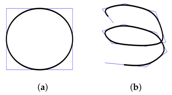
Figure 1. An example of analytic curves produced by application of a generalized subdivision scheme of order 3; (a) circle, (b) helix.

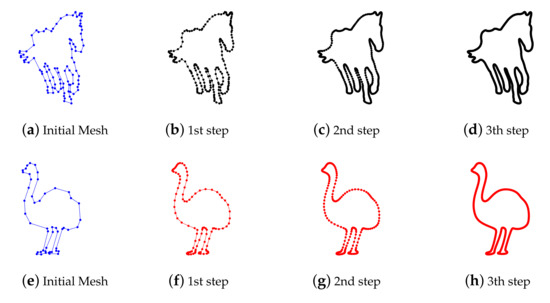
Figure 2. Tree steps of subdivision curves by application of a generalized subdivision scheme of order 3 (black) and 4 (red).

4. Reverse Generalized Subdivision Scheme of Order 3 and Wavelets

In this section we will determine the reverse of the generalized scheme of order 3, then we will give the wavelets corresponding to this scheme.

4.1. Reverse Generalized Subdivision Scheme

Inverse subdivision is the process of finding the coarsest possible representation of a given object by a finer control polygon. In other words, it is a tool that allows us to return to the approximate control polygon of fine data that was obtained by the same direct scheme whose reverse we are looking for or by another scheme. The advantage of the reverse scheme is that it helps us a lot to return to the initial polygon of a fine data easily without losing a lot of time and also without taking a up lot of space because creating a control polygon corresponding to fine data which are very large takes a lot of memory space and this does not happen in the case where the reverse scheme is used. The method for finding the reverse scheme is to take the direct scheme at level ℓ and try to calculate the reverse of that scheme in such a way that we can return to the control polygon $C^{\ell }$ from $C^{\ell +1}$. When we find this reverse scheme, we can apply it ℓ times to easily return to the first control polygon $C^0$. In this subsection, we will use the technique used by Hassan et al. in [29] to extract the reverse scheme corresponding to the generalized scheme of order 3.

By using (2), we have,

$$\left\{\begin{array}{cc}\hfill c_{-2}^{\ell +1}& =c_{-2}^{\ell }\hfill \\ \hfill c_{-1}^{\ell +1}& =\frac{1}{1+u^{\ell }}{c}_{-2}^{\ell }+\frac{u^{\ell }}{1+u^{\ell }}{c}_{-1}^{\ell }\hfill \\ \hfill c_{2i}^{\ell +1}& =\frac{1+2u^{\ell }}{2(1+u^{\ell })}{c}_{i-1}^{\ell }+\frac{1}{2(1+u^{\ell })}{c}_i^{\ell },i=0,\dots ,2^{\ell }-2\hfill \\ \hfill c_{2i+1}^{\ell +1}& =\frac{1}{2(1+u^{\ell })}{c}_{i-1}^{\ell }+\frac{1+2u^{\ell }}{2(1+u^{\ell })}{c}_i^{\ell },i=0,\dots ,2^{\ell }-2\hfill \\ \hfill c_{2^{\ell +1}-2}^{\ell +1}& =\frac{u^{\ell }}{1+u^{\ell }}{c}_{2^{\ell }-2}^{\ell }+\frac{1}{1+u^{\ell }}{c}_{2^{\ell }-1}^{\ell }\hfill \\ \hfill c_{2^{\ell +1}-1}^{\ell +1}& =c_{2^{\ell }-1}^{\ell }\hfill \end{array}\right.$$

(4)

The components of vector $C^{\ell }$ are determined from the system (4), as follows:

$$\left\{\begin{array}{cc}\hfill c_{-2}^{\ell }& =c_{-2}^{\ell +1}\hfill \\ \hfill c_{-1}^{\ell }& =\frac{-1}{u^{\ell }}{c}_{-2}^{\ell +1}+\frac{1+u^{\ell }}{u^{\ell }}{c}_{-1}^{\ell +1}\hfill \\ \hfill c_{2^{\ell }-2}^{\ell }& =\frac{1+u^{\ell }}{u^{\ell }}{c}_{2^{\ell +1}-2}^{\ell +1}-\frac{1}{u^{\ell }}{c}_{2^{\ell +1}-1}^{\ell +1}\hfill \\ \hfill c_{2^{\ell }-1}^{\ell }& =c_{2^{\ell +1}-1}^{\ell +1}\hfill \end{array}\right.$$

(5)

and for $i=0,\cdots ,2^{\ell -1}-2$ we have

$$\left\{\begin{array}{c}{c}_{i-1}^{\ell }=\frac{1+2u^{\ell }}{2u^{\ell }}{c}_{2i}^{\ell +1}-\frac{1}{2u^{\ell }}{c}_{2i+1}^{\ell +1}\hfill \\ c_i^{\ell }=-\frac{1}{2u^{\ell }}{c}_{2i}^{\ell +1}+\frac{1+2u^{\ell }}{2u^{\ell }}{c}_{2i+1}^{\ell +1}.\hfill \end{array}\right.$$

In order to determine the stages of the forward–backward subdivision patterns, it is sufficient to take the average of the two positions and to store the error vectors (see [29]).

Consequently, for $i=0,\cdots ,2^{\ell -1}-3$,

$$\left\{\begin{array}{cc}\hfill c_i^{\ell }& =-\frac{1}{4u^{\ell }}{c}_{2i}^{\ell +1}+\frac{1+2u^{\ell }}{4u^{\ell }}{c}_{2i+1}^{\ell +1}+\frac{1+2u^{\ell }}{4u^{\ell }}{c}_{2i+2}^{\ell +1}-\frac{1}{4u^{\ell }}{c}_{2i+3}^{\ell +1}\hfill \\ \hfill d_i^{\ell }& =\frac{1}{4u^{\ell }}{c}_{2i}^{\ell +1}-\frac{1+2u^{\ell }}{4u^{\ell }}{c}_{2i+1}^{\ell +1}+\frac{1+2u^{\ell }}{4u^{\ell }}{c}_{2i+2}^{\ell +1}-\frac{1}{4u^{\ell }}{c}_{2i+3}^{\ell +1}\hfill \end{array}\right.$$

(6)

where $d_i^{\ell }$ is the detail values that can be used to reconstruct the data $c^{\ell +1}$. The vector that gathers these values denoted by $D^{\ell }$ and is called the detail vector.

Moreover,

$$\left\{\begin{array}{cc}\hfill c_{-2}^{\ell }& =c_{-2}^{\ell +1}\hfill \\ \hfill d_{-2}^{\ell }& =0\hfill \\ \hfill c_{-1}^{\ell }& =\frac{-1}{2u^{\ell }}{c}_{-2}^{\ell +1}+\frac{1+u^{\ell }}{2u^{\ell }}{c}_{-1}^{\ell +1}+\frac{1+2u^{\ell }}{4u^{\ell }}{c}_0^{\ell +1}-\frac{1}{4u^{\ell }}{c}_1^{\ell +1}\hfill \\ \hfill d_{-1}^{\ell }& =\frac{1}{2u^{\ell }}{c}_{-2}^{\ell +1}-\frac{1+u^{\ell }}{2u^{\ell }}{c}_{-1}^{\ell +1}+\frac{1+2u^{\ell }}{4u^{\ell }}{c}_0^{\ell +1}-\frac{1}{4u^{\ell }}{c}_1^{\ell +1}\hfill \\ \hfill c_{2^{\ell }-2}^{\ell }& =-\frac{1}{4u^{\ell }}{c}_{2^{\ell +1}-4}^{\ell +1}+\frac{1+2u^{\ell }}{4u^{\ell }}{c}_{2^{\ell +1}-3}^{\ell +1}+\frac{1+u^{\ell }}{2u^{\ell }}{c}_{2^{\ell +1}-2}^{\ell +1}-\frac{1}{2u^{\ell }}{c}_{2^{\ell +1}-1}^{\ell +1}\hfill \\ \hfill d_{2^{\ell }-2}^{\ell }& =-\frac{1}{4u^{\ell }}{c}_{2^{\ell +1}-4}^{\ell +1}+\frac{1+2u^{\ell }}{4u^{\ell }}{c}_{2^{\ell +1}-3}^{\ell +1}-\frac{1+u^{\ell }}{2u^{\ell }}{c}_{2^{\ell +1}-2}^{\ell +1}+\frac{1}{2u^{\ell }}{c}_{2^{\ell +1}-1}^{\ell +1}\hfill \\ \hfill c_{2^{\ell }-1}^{\ell }& =c_{2^{\ell +1}-1}^{\ell +1}\hfill \\ \hfill d_{2^{\ell }-1}^{\ell }& =0,\hfill \end{array}\right.$$

(7)

Consequently, for $i=0,\dots ,2^{\ell }-3$

$$\left\{\begin{array}{cc}\hfill c_{-2}^{\ell +1}& =c_{-2}^{\ell }\hfill \\ \hfill c_{-1}^{\ell +1}& =\frac{1}{1+u^{\ell }}{c}_{-2}^{\ell }+\frac{u^{\ell }}{1+u^{\ell }}(c_{-1}^{\ell }-d_{-1})\hfill \\ \hfill c_{2i}^{\ell +1}& =\frac{1+2u^{\ell }}{2(1+u^{\ell })}\left(c_{i-1}^{\ell }-d_{i-1}^{\ell }\right)+\frac{1}{2(1+u^{\ell })}\left(c_i^{\ell }+d_i^{\ell }\right)\hfill \\ \hfill c_{2i+1}^{\ell +1}& =\frac{1}{2(1+u^{\ell })}\left(c_{i-1}^{\ell }-d_{i-1}^{\ell }\right)+\frac{1+2u^{\ell }}{2(1+u^{\ell })}\left(c_i^{\ell }+d_i^{\ell }\right)\hfill \\ \hfill c_{2^{\ell +1}-2}^{\ell +1}& =\frac{u^{\ell }}{1+u^{\ell }}(c_{2^{\ell }-2}-d_{2^{\ell }-2})+\frac{1}{1+u^{\ell }}{c}_{2^{\ell }-1}^{\ell }\hfill \\ \hfill c_{2^{\ell +1}-1}^{\ell +1}& =c_{2^{\ell }-1}^{\ell }.\hfill \end{array}\right.$$

(8)

Remark 2.

• When $u^{\ell }=1$ this reverse generalized scheme becomes the reverse of the Chaikin scheme proposed in [29].
• In the reverse step from level $\ell +1$ to level ℓ, the tension parameter is updated as follows:

  $$u^{\ell }=2{\left(u^{\ell +1}\right)}^2-1.$$

4.2. Numerical Example

To show the added value of our inverse generalized subdivision scheme, we propose in this section some examples related to trigonometric and hyperbolic curves. Indeed, In Figure 3 we apply three levels step of reverse generalized subdivision scheme of order 3 to limit form (blue) with values of the tension parameter equal to $1.2$. In Figure 4 we show the advantage of the generalized reverse scheme of order 3 in the reconstruction of original initial control polygonal trigonometric form and hyperbolic form. The tension parameters applied are $0.9$ and $1.12$.

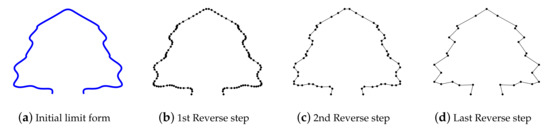
Figure 3. An open curve and their three levels of generalized B-spline reverse subdivision of order 3.

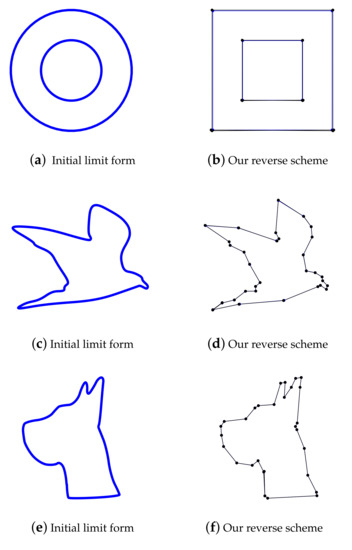
Figure 4. The generalized reverse scheme of order 3.

It is well known that the multi-resolution process of a subdivision model allows increase or decrease in the resolution of a given mesh. For example, in animated films, we use meshes that are too smooth when the images are close together and coarse meshes in the opposite case (see [31]).

4.3. Multiresolution and Reverse Subdivision Scheme

The objective of this section is to construct generalized spline wavelets associated with generalized splines of order 3 with multiple nodes at the edges of the interval [a,b].

Let $F^{\ell }$ be a set of fine points. The multi-resolution decomposition of $F^{\ell }$ and given by:

$$C^{\ell }=A_3^{\ell }{F}^{\ell }\mathrm{and}{D}^{\ell }=B_3^{\ell }{F}^{\ell },$$

where

• $C^{\ell }$ is a set of coarse points;
• $D^{\ell }$ is a set of detailed points;
• $A_3^{\ell }$ and $B_3^{\ell }$ are the filters matrix of size $\left(2^{\ell }+2\right)\times \left(2^{\ell +1}+2\right).$

According to (6) it is easy to find that:

$$A_3^{\ell }=\left(\begin{array}{cccccccccc}1& 0& 0& 0& 0& 0& \cdots & 0& 0& 0\\ -\frac{1}{2u^{\ell }}& \frac{1+u^{\ell }}{2u^{\ell }}& \frac{1+2u^{\ell }}{4u^{\ell }}& -\frac{1}{4u^{\ell }}& 0& 0& \cdots & 0& 0& 0\\ 0& 0& -\frac{1}{4u^{\ell }}& \frac{1+2u^{\ell }}{2u^{\ell }}& \frac{1+2u^{\ell }}{2u^{\ell }}& -\frac{1}{4u^{\ell }}& 0& \cdots & 0& 0\\ ⋮& ⋮& 0& \ddots & \ddots & \ddots & \ddots & ⋮& ⋮& ⋮\\ ⋮& ⋮& ⋮& 0& -\frac{1}{4u^{\ell }}& \frac{1+2u^{\ell }}{2u^{\ell }}& \frac{1+2u^{\ell }}{2u^{\ell }}& -\frac{1}{4u^{\ell }}& 0& 0\\ ⋮& ⋮& ⋮& ⋮& 0& 0& -\frac{1}{4u^{\ell }}& \frac{1+2u^{\ell }}{4u^{\ell }}& \frac{1+u^{\ell }}{2u^{\ell }}& -\frac{1}{2u^{\ell }}\\ 0& 0& 0& 0& 0& 0& 0& 0& 0& 1\end{array}\right),$$

$$B_3^{\ell }=\left(\begin{array}{cccccccccc}0& 0& 0& 0& 0& 0& \cdots & 0& 0& 0\\ \frac{1}{2u^{\ell }}& -\frac{1+u^{\ell }}{2u^{\ell }}& \frac{1+2u^{\ell }}{4u^{\ell }}& -\frac{1}{4u^{\ell }}& 0& 0& \cdots & 0& 0& 0\\ 0& 0& \frac{1}{4u^{\ell }}& -\frac{1+2u^{\ell }}{2u^{\ell }}& \frac{1+2u^{\ell }}{2u^{\ell }}& -\frac{1}{4u^{\ell }}& 0& \cdots & 0& 0\\ ⋮& ⋮& 0& \ddots & \ddots & \ddots & \ddots & ⋮& ⋮& ⋮\\ ⋮& ⋮& ⋮& 0& \frac{1}{4u^{\ell }}& -\frac{1+2u^{\ell }}{2u^{\ell }}& \frac{1+2u^{\ell }}{2u^{\ell }}& -\frac{1}{4u^{\ell }}& 0& 0\\ ⋮& ⋮& ⋮& ⋮& 0& 0& -\frac{1}{4u^{\ell }}& \frac{1+2u^{\ell }}{4u^{\ell }}& -\frac{1+u^{\ell }}{2u^{\ell }}& \frac{1}{2u^{\ell }}\\ 0& 0& 0& 0& 0& 0& 0& 0& 0& 0\end{array}\right),$$

The reconstruction can be obtained by using the synthesis filters $P_3^{\ell }$ and $Q_3^{\ell }$ such that $F^{\ell }={\mathcal{P}}_3^{\ell }{C}^{\ell }+Q_3^{\ell }{D}^{\ell }$. From the Formula (8), the matrix $Q_3^{\ell }$ is defined as follow

$$Q_3^{\ell }=\left(\begin{array}{cccccccc}1& 0& 0& 0& \cdots & 0& 0& 0\\ \frac{1}{1+u^{\ell }}& \frac{u^{\ell }}{1+u^{\ell }}& 0& 0& 0& 0\\ 0& \frac{1+2u^{\ell }}{2(1+u^{\ell })}& \frac{1}{2(1+u^{\ell })}& 0& \cdots & 0& 0& 0\\ 0& \frac{1}{2(1+u^{\ell })}& \frac{1+2u^{\ell }}{2(1+u^{\ell })}& 0& \cdots & 0& 0& 0\\ 0& 0& \frac{1+2u^{\ell }}{2(1+u^{\ell })}& \frac{1}{2(1+u^{\ell })}& \cdots & 0& 0& 0\\ 0& 0& \frac{1}{2(1+u^{\ell })}& \frac{1+2u^{\ell }}{2(1+u^{\ell })}& \cdots & 0& 0& 0\\ ⋮& ⋮& ⋮& ⋮& \ddots & ⋮& ⋮& ⋮\\ 0& 0& 0& 0& \cdots & \frac{1+2u^{\ell }}{2(1+u^{\ell })}& \frac{1}{2(1+u^{\ell })}& 0\\ 0& 0& 0& 0& \cdots & \frac{1}{2(1+u^{\ell })}& \frac{1+2u^{\ell }}{2(1+u^{\ell })}& 0\\ 0& 0& 0& 0& \cdots & 0& \frac{u^{\ell }}{1+u^{\ell }}& \frac{1}{1+u^{\ell }}\\ 0& 0& 0& 0& \cdots & \cdots & 0& 1\end{array}\right),$$

where $dim\left(Q_3^{\ell }\right)=\left(2^{\ell +1}+2\right)\times \left(2^{\ell }+2\right).$

Consequently, using the matrix $Q_3^{\ell }$, the generalized B-wavelets ${\psi }_{i,\ell -1}$ are given by:

$$\begin{array}{cc}\hfill & {\psi }_{-2,\ell -1}=N_{-2,3}\left(\varphi \right),\hfill \\ \hfill & {\psi }_{-1,\ell -1}=\frac{1}{1+u^{\ell }}{N}_{-2,3}\left(\varphi \right)-\frac{u^{\ell }}{1+u^{\ell }}{N}_{-1,3}\left(\varphi \right)+\frac{u^{\ell }}{1+u^{\ell }}{N}_{0,3}\left(\varphi \right),\hfill \end{array}$$

${\psi }_{i,\ell -1}=\frac{1}{2(1+u^{\ell })}\left(N_{2i,3}\left(\varphi \right)-N_{2i+3,3}\left(\varphi \right)\right)+\frac{1+2u^{\ell }}{2(1+u^{\ell })}\left(N_{2i+2,3}\left(\varphi \right)-N_{2i+1,3}\left(\varphi \right)\right),i=0,\dots ,2^{\ell -1}-3,$

$$\begin{array}{cc}\hfill & {\psi }_{2^{\ell -1}-2,\ell -1}=\frac{u^{\ell }}{1+u^{\ell }}{N}_{2^{\ell }-3,3}\left(\varphi \right)-\frac{u^{\ell }}{1+u^{\ell }}{N}_{2^{\ell }-2,3}\left(\varphi \right)+\frac{1}{1+u^{\ell }}{N}_{2^{\ell }-1,3}\left(\varphi \right)\hfill \\ \hfill & {\psi }_{2^{\ell -1}-1,\ell -1}=N_{2^{\ell }-1,3}\left(\varphi \right).\hfill \end{array}$$

In Figure 5, we give an example of the generalized B-wavelettes ${\psi }_{i,\ell -1}$ of order 3, for $u^0=0.7$ (Blue line), $u^0=1$ (Magenta line), $u^0=1.32$ (Red line).

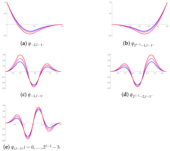
Figure 5. Graphs of Generalized B-spline wavelets for $u^0=0.7$ (Blue line), $u^0=1$ (Magenta line) and $u^0=1.32$ (Red line).

5. Reverse Generalized Subdivision Scheme of Order 4

The method used to reverse the subdivision scheme of order 3 cannot be applied to find the reverse of the generalized subdivision of order 4. For this reason, in this Section, we present two methods: the first one is based on the least-squares formulation that is presented in [32] while the second one is based on solving the minimization of linear optimization problems.

5.1. Least-Squares Formulation

Since $P_4^{\ell }$ is not a square matrix then ${\left(P_4^{\ell }\right)}^{-1}$ does not exist. However, using the same technique presented in [32], we will find a reverse scheme of order 4. Indeed, to compute the different components of the multiresolution structure we adopt the constrained wavelet approach proposed by L. Olsen et al. (see [32]). The described approach uses the link between the even and odd rules of the subdivision filters. It starts by determining the decomposition and reconstruction matrices tests which are equal in our case    

$${\tilde{A}}_4^{\ell }=\left(\begin{array}{ccccccccc}1& 0& 0& 0& 0& \cdots & 0& 0& 0\\ \frac{-1}{u^{\ell }}& \frac{1+u^{\ell }}{u^{\ell }}& 0& 0& 0& \cdots & 0& 0& 0\\ 0& \frac{-1}{2u^{\ell }}& \frac{1+u^{\ell }}{u^{\ell }}& \frac{-1}{2u^{\ell }}& \cdots & 0& 0& 0& 0\\ ⋮& ⋮& ⋮& ⋮& \ddots & ⋮& ⋮& ⋮& ⋮\\ 0& 0& 0& 0& \cdots & \frac{-1}{2u^{\ell }}& \frac{1+u^{\ell }}{u^{\ell }}& \frac{-1}{2u^{\ell }}& 0\\ 0& 0& 0& 0& \cdots & 0& 0& \frac{1+u^{\ell }}{u^{\ell }}& \frac{-1}{u^{\ell }}\\ 0& 0& 0& 0& \cdots & 0& 0& \cdots & 1\end{array}\right),$$

$${\tilde{Q}}_4^{\ell }=\left(\begin{array}{ccccc}0& 0& \cdots & 0& 0\\ 0& 0& \cdots & 0& 0\\ 1& 0& \cdots & 0& 0\\ \frac{1}{2(1+u^{\ell })}& \frac{1}{2(1+u^{\ell })}& \cdots & 0& 0\\ ⋮& ⋮& \ddots & ⋮& ⋮\\ 0& \cdots & 0& \frac{1}{2(1+u^{\ell })}& \frac{1}{2(1+u^{\ell })}\\ 0& \cdots & 0& 0& 1\\ 0& \cdots & 0& 0& 0\\ 0& \cdots & 0& \cdots & 0\end{array}\right),$$

$${\tilde{B}}_4^{\ell }=\left(\begin{array}{cccccccccc}\frac{1+2u^{\ell }}{4u^{\ell }}& -\frac{1+2u^{\ell }}{2u^{\ell }}& \frac{1+8u^{\ell }}{8u^{\ell }}& \frac{-1}{2u^{\ell }}& \frac{1}{8u^{\ell }}& 0& \cdots & 0& 0& 0\\ 0& \frac{1}{4u^{\ell }}& -\frac{1+u^{\ell }}{u^{\ell }}& \frac{1+2u^{\ell }}{u^{\ell }}& -\frac{1+u^{\ell }}{u^{\ell }}& \frac{1}{4u^{\ell }}& \cdots & 0& 0& 0\\ ⋮& ⋮& ⋮& ⋮& ⋮& ⋮& \ddots & ⋮& ⋮& ⋮\\ 0& 0& 0& \cdots & \frac{1}{4u^{\ell }}& -\frac{1+u^{\ell }}{u^{\ell }}& \frac{1+2u^{\ell }}{u^{\ell }}& -\frac{1+u^{\ell }}{u^{\ell }}& \frac{1}{4u^{\ell }}& 0\\ 0& 0& 0& \cdots & 0& \frac{1}{8u^{\ell }}& \frac{-1}{2u^{\ell }}& \frac{1+8u^{\ell }}{8u^{\ell }}& -\frac{1+2u^{\ell }}{2u^{\ell }}& \frac{1+2u^{\ell }}{4u^{\ell }}\end{array}\right).$$

Secondly, as described in [32], these three matrices cannot allow us to return to the original mesh $C^{\ell }$, and the error denoted by ${\Delta }_4^{\ell }$ between the original point $C^{\ell }$ and what is given by application of these matrices denoted by ${\tilde{C}}^{\ell }$ is very large. To this end, the authors solved this problem by minimizing the least-squares error metric and they showed in the proof that the values of ${\Delta }_4^{\ell }$ can be calculated by determination of matrix $L_4^{\ell }$ such that ${\Delta }^{\ell }=L_4^{\ell }{\tilde{D}}^{\ell }$. The values of the matrix $L_4^{\ell }$ is

$$L_4^{\ell }=\left(\begin{array}{ccccc}0& 0& \cdots & 0& 0\\ 0& 0& \cdots & 0& 0\\ {\mu }^{\ell }& {\mu }^{\ell }& \cdots & 0& 0\\ 0& {\mu }^{\ell }& {\mu }^{\ell }& \cdots & 0\\ ⋮& ⋮& \ddots & ⋮& ⋮\\ 0& \cdots & {\mu }^{\ell }& {\mu }^{\ell }& 0\\ 0& \cdots & 0& {\mu }^{\ell }& {\mu }^{\ell }\\ 0& \cdots & 0& \cdots & 0\\ 0& \cdots & 0& \cdots & 0\end{array}\right)$$

with ${\mu }^{\ell }=\frac{(1+2u^{\ell })(1+6u^{\ell }+2{\left(u^{\ell }\right)}^2)}{2(1+u^{\ell })(3+8u^{\ell }+6{\left(u^{\ell }\right)}^2)}.$

Remark 3.

• The matrices ${\tilde{A}}_4^{\ell },{\tilde{Q}}_4^{\ell },{\tilde{B}}_4^{\ell }$ and $L_4^{\ell }$ above are calculated by using the same steps for calculating matrices $\tilde{A},\tilde{Q},\tilde{B}$ and L in [32].
• When $u^{\ell }=1$ this reverse generalized scheme becomes the reverse of cubic scheme that is proposed in [32].

5.2. Linear Optimization Problem

In this subsection, we present another method to calculate the same error ${\Delta }_4^{\ell }$ but this time as a function of $P_4^{\ell }$. In fact, this method starts from a subdivision matrix $P_4^{\ell }$. The concept is to use the given subdivision scheme $P_4^{\ell }$ to obtain the better $A_4^{\ell }$ that produces coarse points with minimal subdivision error. The coefficients of the weak resolution $C^{\ell }$ are obtained by minimizing the distance between $P_4^{\ell }{C}^{\ell }$ and $F^{\ell }$. This leads to:

$$E\left(C^{\ell }\right)={\parallel P_4^{\ell }{C}^{\ell }-F^{\ell }\parallel }_2^2.$$

(9)

Thus,

$$\begin{array}{cc}\hfill E\left(C^{\ell }\right)& ={(P_4^{\ell }{C}^{\ell }-F^{\ell })}^T(P_4^{\ell }{C}^{\ell }-F^{\ell })\hfill \\ \hfill & ={\left(F^{\ell }\right)}^T{F}^{\ell }-2{\left(C^{\ell }\right)}^T{\left(P_4^{\ell }\right)}^T{F}^{\ell }+{\left(C^{\ell }\right)}^T{\left(P_4^{\ell }\right)}^T{P}_4^{\ell }{C}^{\ell }.\hfill \end{array}$$

(10)

The first derivative of Equation (10) is

$$\nabla E\left(C^{\ell }\right)=-2{\left(P_4^{\ell }\right)}^T{F}^{\ell }+2{\left(P_4^{\ell }\right)}^T{P}_4^{\ell }{C}^{\ell }$$

and the second derivative is

$${\nabla }^{2}E\left(C^{\ell }\right)=2{\left(P_4^{\ell }\right)}^T{P}_4^{\ell }.$$

As the 2nd derivative is symmetrically positive definite, the solution of Equation (9) is a local minimum. Thus, for $\nabla E\left(C^{\ell }\right)=0,$ we obtain

$${\left(P_4^{\ell }\right)}^T{P}_4^{\ell }{C}^{\ell }={\left(P_4^{\ell }\right)}^T{F}^{\ell },$$

(11)

since $C^{\ell }=A_4^{\ell }{F}^{\ell }$, solving normal Equation (11) for $C^{\ell }$ provides

$$A_4^{\ell }={\left({\left(P_4^{\ell }\right)}^T{P}_4^{\ell }\right)}^{-1}{\left(P_4^{\ell }\right)}^T,$$

$$E({\tilde{C}}^{\ell }+{\Delta }_4^{\ell })={\parallel F^{\ell }-P_4^{\ell }({\tilde{C}}^{\ell }+{\Delta }_4^{\ell })\parallel }_2^2.$$

It yields with (11),

$$\left({\left(P_4^{\ell }\right)}^T{P}_4^{\ell }\right)({\tilde{C}}^{\ell }+{\Delta }_4^{\ell })={\left(P_4^{\ell }\right)}^T{F}^{\ell }.$$

(12)

Replacing $F^{\ell }$ by $P_4^{\ell }{\tilde{C}}^{\ell }+{\tilde{Q}}_4^{\ell }{\tilde{D}}^{\ell }$ and simplifying shows that equality (12) is equivalent to

$$\left({\left(P_4^{\ell }\right)}^T{P}_4^{\ell }\right){\Delta }_4^{\ell }={\left(P_4^{\ell }\right)}^T{\tilde{Q}}_4^{\ell }{\tilde{D}}^{\ell }.$$

(13)

Then ${\Delta }_4^{\ell }$ can be computed from the above linear system.

5.3. Numerical Example

In this subsection, we give examples of using our approach in synthesizing applications.

Figure 6 presents the powerful generalized reverse subdivision scheme of order 4 to reproduce a different initial control polygonal. The tension parameter for the dog is $0.9$ where the one chosen for the head is $1.1$.

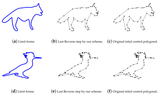
Figure 6. The generalized reverse scheme of order 4.

The Algorithm 1 summarizes the decomposition process of $F^{\ell }$.

Algorithm 1: Decomposition

6. Conclusions

In this paper, we have constructed a reverse generalized subdivision scheme of order 3 and 4 by two different methods. In comparison with other existing methods in the literature, our proposed reverse scheme can reproduce exactly the initial control polygonal of trigonometric and hyperbolic forms. A multiresolution representation based on a reverse subdivision approach which has interesting applications is also studied in this paper.

References

- De Rham, G. Sur une courbe plane. J. Math. Pures Appl. 1956, 35, 25–42. [Google Scholar]
- Beccari, C.; Casciola, G.; Romani, L. A non-stationary uniform tension controlled interpolating 4-point scheme reproducing conics. Comput. Aided Geom. Des. 2007, 24, 1–9. [Google Scholar] [CrossRef]
- Daniel, S.; Shunmugaraj, P. An approximating C2 non-stationary subdivision scheme. Comput. Aided Geom. Des. 2009, 26, 810–821. [Google Scholar] [CrossRef]
- Daniel, S.; Shunmugaraj, P. Some interpolating non-stationary subdivision schemes. In Proceedings of the 2011 International Symposium on Computer Science and Society, Kota Kinabalu, Malaysia, 16–17 July 2011; pp. 400–403. [Google Scholar]
- Fang, M.-E.; Ma, W.; Wang, G. A generalized curve subdivision scheme of arbitrary order with a tension parameter. Comput. Aided Geom. Des. 2010, 27, 720–733. [Google Scholar] [CrossRef]
- Dyn, N.; Levin, D. Subdivision schemes in geometric modelling. Acta Numer. 2002, 11, 73–144. [Google Scholar] [CrossRef]
- Salomon, D. Curves and Surfaces for Computer Graphics; Springer: New York, NY, USA, 2006. [Google Scholar]
- Warren, J.; Weimer, H. Subdivision Methods for Geometric Design—A Constructive Approach; Morgan-Kaufmann Publishers: San Francisco, CA, USA, 2002. [Google Scholar]
- Lipovetsky, E. Subdivision of point-normal pairs with application to smoothing feasible robot path. Vis. Comput. 2021. [Google Scholar] [CrossRef]
- Badoual, A.; Schmitter, D.; Uhlmann, V.; Unser, M. Multiresolution subdivision snakes. IEEE Trans. Image Process. 2016, 26, 1188–1201. [Google Scholar] [CrossRef]
- Conti, C.; Romani, L.; Unser, M. Ellipse-preserving Hermite interpolation and subdivision. J. Math. Anal. Appl. 2015, 426, 211–227. [Google Scholar] [CrossRef]
- Schmitter, D.; Fageot, J.; Badoual, A.; Garcia-Amorena, P.; Unser, M. Compactly-supported smooth interpolators for shape modeling with varying resolution. Graph. Models 2017, 94, 52–64. [Google Scholar] [CrossRef]
- Amat, S.; Donat, R.; Liandrat, J.; Trillo, J.C. A fully adaptive PPH multiresolution scheme for image processing. Math. Comput. Model. 2007, 46, 2–11. [Google Scholar] [CrossRef]
- Amat, S.; Liandrat, J. Nonlinear thresholding of multiresolution decompositions adapted to the presence of discontinuities. Adv. Comput. Math. 2013, 38, 133–146. [Google Scholar] [CrossRef][Green Version]
- Bartels, R.; Samavati, F. Multiresolutions numerically from subdivisions. Comput. Graph. 2011, 35, 185–197. [Google Scholar] [CrossRef]
- Bartels, R.; Samavati, F. Reversing subdivision rules: Local linear conditions and observations on inner products. J. Comput. Appl. Math. 2000, 119, 29–67. [Google Scholar] [CrossRef][Green Version]
- Charina, M.; Conti, C. Polynomial reproduction of multivariate scalar subdivision schemes. J. Comput. Appl. Math. 2013, 240, 51–61. [Google Scholar] [CrossRef]
- Charina, M.; Conti, C.; Guglielmi, N.; Protasov, V. Regularity of non-stationary multivariate subdivision: A matrix approach. Numer. Math. 2017, 135, 639–678. [Google Scholar] [CrossRef]
- Charina, M.; Conti, C.; Jetter, K.; Zimmermann, G. Scalar multivariate subdivision schemes and box splines. Comput. Aided Geom. Des. 2011, 28, 285–306. [Google Scholar] [CrossRef]
- Romani, L. From approximating subdivision schemes for exponential splines to high-performance interpolating algorithms. J. Comput. Appl. Math 2009, 224, 383–396. [Google Scholar] [CrossRef]
- Ghaffar, A.; Ullah, Z.; Bari, M.; Nisar, K.S.; Al-Qurashi, M.M.; Baleanu, D. A new class of 2 m-point binary non-stationary subdivision schemes. Adv. Differ. Equ. 2019, 2019, 325. [Google Scholar] [CrossRef]
- Fakhar, R.; Lamnii, A.; Nour, M.-Y.; Zidina, A. Mixed trigonometric and hyperbolic subdivision scheme with two tension and one shape parameters. Int. J. Comput. Math. 2021. [Google Scholar] [CrossRef]
- Fakhar, R.; Lamnii, A.; Nour, M.-Y.; Zidina, A. Mixed hyperbolic/trigonometric non-stationary subdivision scheme. Math. Sci. 2021. [Google Scholar] [CrossRef]
- Siddiqi, S.S.; Salam, W.; Rehan, K. Binary 3-point and 4-point non-stationary subdivision schemes using hyperbolic function. Appl. Math. Comput. 2015, 258, 120–129. [Google Scholar] [CrossRef]
- Siddiqi, S.S.; Salam, W.; Rehan, K. A new non-stationary binary 6-point subdivision scheme. Appl. Math. Comput. 2015, 268, 1227–1239. [Google Scholar] [CrossRef]
- Foster, K.; Sousa, M.C.; Samavati, F.F.; Wyvill, B. Polygonal silhouette error correction: A reverse subdivision approach. Int. J. Comput. Eng. 2007, 3, 53–70. [Google Scholar] [CrossRef]
- Mündermann, L.; MacMurchy, P.; Pivovarov, J.; Prusinkiewicz, P. Modeling lobed leaves. In Proceedings of the Computer Graphics International 2003, Tokyo, Japan, 9–11 July 2003; pp. 60–65. [Google Scholar]
- Sadeghi, J.; Samavati, F.F. Smooth reverse Loop and Catmull-Clark subdivision. Graph. Models 2011, 73, 202–217. [Google Scholar] [CrossRef]
- Dodgson, N.A.; Hassan, M.F. Reverse Subdivision. In Advances in Multiresolution for Geometric Modelling; Springer: Berlin/Heidelberg, Germany, 2005; pp. 271–283. [Google Scholar]
- Dyn, N.; Zhuang, X. Linear multiscale transforms based on even-reversible subdivision operators. In Excursions in Harmonic Analysis; Springer: Berlin/Heidelberg, Germany, 2020; Volume 6. [Google Scholar]
- Ajeddar, M.; Lamnii, A. Smooth reverse subdivision of uniform algebraic hyperbolic B-splines and wavelets. Int. J. Wavelets Multiresolut. Inf. Process. 2021. [Google Scholar] [CrossRef]
- Olsen, L.; Samavati, F.F.; Bartels, R.H. Multiresolution for curves and surfaces based on constraining wavelets. Comput. Graph. 2007, 31, 449–462. [Google Scholar] [CrossRef]
- Xu, G.; Wang, G. AHT Bézier Curves and NUAHT B-Spline Curves. J. Comput. Sci. Technol. 2007, 22, 597–607. [Google Scholar] [CrossRef]
- Conti, C.; Dyn, N. Non-stationary Subdivision Schemes: State of the Art and Perspectives. In Approximation Theory XVI at 2019; Fasshauer, G.E., Neamtu, M., Schumaker, L.L., Eds.; Springer Proceedings in Mathematics and Statistics; Springer: Cham, Switzerland, 2021; Volume Voumle 336, pp. 39–71. [Google Scholar]
- Conti, C.; Gemignani, L.; Romani, L. Exponential Pseudo-Splines: Looking beyond Exponential B-splines. J. Math. Anal. Appl. 2016, 439, 32–56. [Google Scholar] [CrossRef]
Publisher’s Note: MDPI stays neutral with regard to jurisdictional claims in published maps and institutional affiliations. |
© 2021 by the authors. Licensee MDPI, Basel, Switzerland. This article is an open access article distributed under the terms and conditions of the Creative Commons Attribution (CC BY) license (https://creativecommons.org/licenses/by/4.0/).