
Structural Optimization and Application Research of Alkali-Activated Slag Ceramsite Compound Insulation Block Based on Finite Element Method

Abstract
:1. Introduction
- Six types of AASCCIBs with different internal structures are designed based on different numbers of hole rows and hole ratios.
- Based on the FEM, the thermal and mechanical performances of six AASCCIBs are simulated using ANSYS CFX. Moreover, the AASCCIB with the optimal comprehensive performance is determined though a multi-objective optimization analysis.
- The improvement effect of the AASCCIB wall on the indoor thermal environment relative to an ordinary block (OB) wall is quantitatively analyzed using ANSYS CFX.
2. Methods
2.1. Structural Design of AASCCIBs
2.2. Numerical Simulation of Thermal and Mechanical Performances of AASCCIBs
2.2.1. Mathematical Model
2.2.2. Development of the Finite Element Model
- 1.
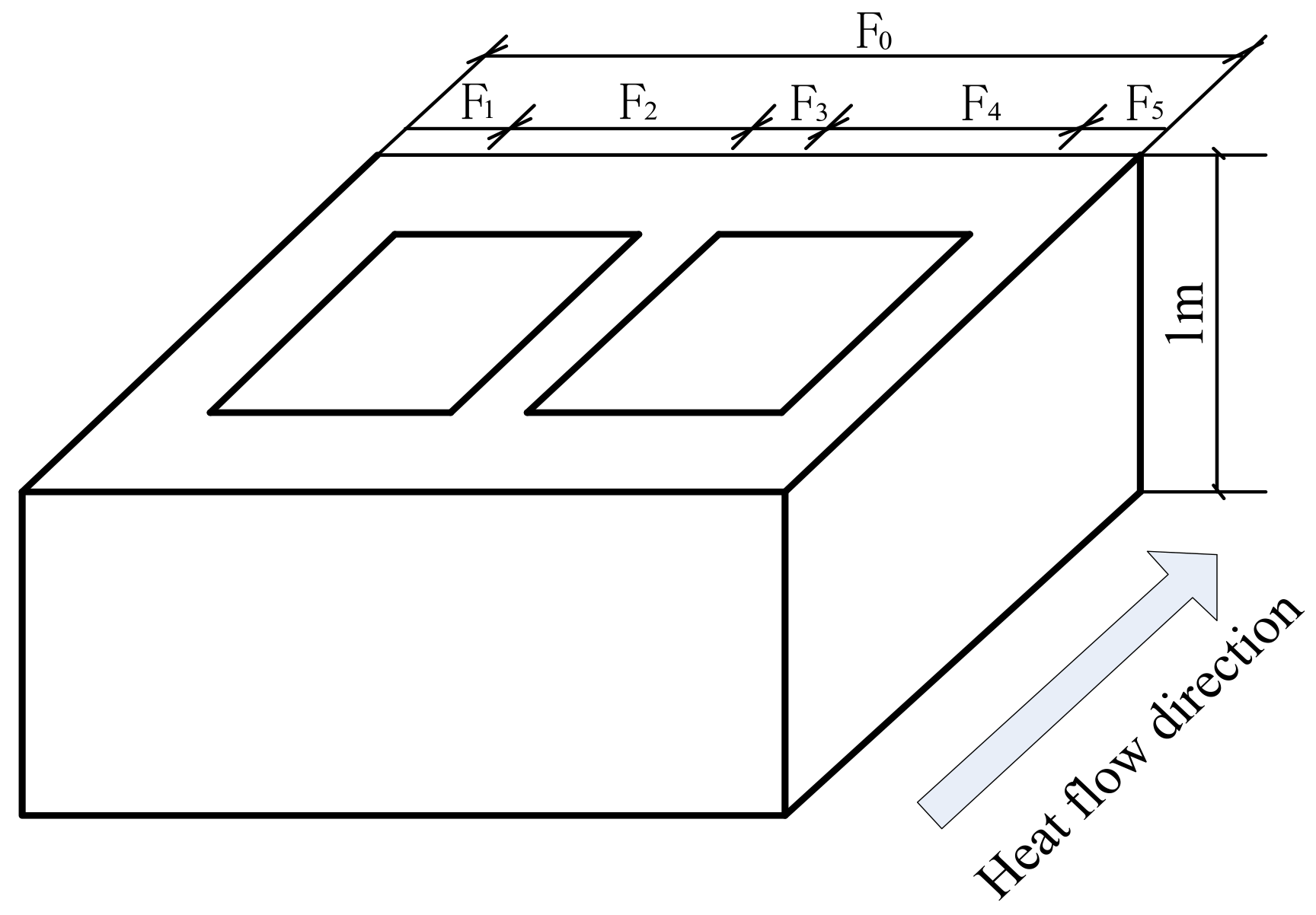
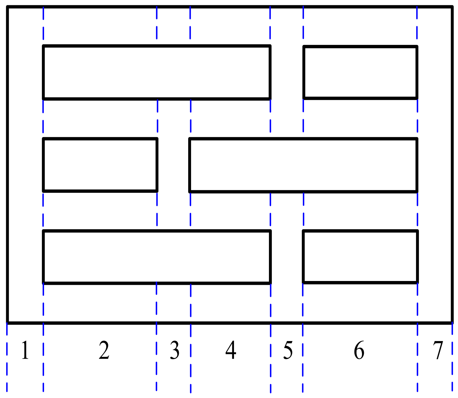
- Basic assumptions and geometric modelThe following assumptions were used before the thermal model was developed:
- (1)
- The block performs a one-dimensional heat transfer.
- (2)
- The temperatures on both sides of the block are constant.
- (3)
- The main material of block and the filling material are closely connected. The material performances do not vary with the thermal environment.
- 2.
- Mesh division
- 3.
- Material parameter and boundary condition setting
2.3. Multi-Objective Optimization of AASCCIBs
2.3.1. Multi-Objective Optimization Method
2.3.2. Calculation of the Weight Coefficient
2.3.3. Factor Normalization
2.4. Influence of AASCCIB Wall on the Indoor Thermal Environment
2.4.1. Mathematical Model
2.4.2. Development of the Finite Element Model
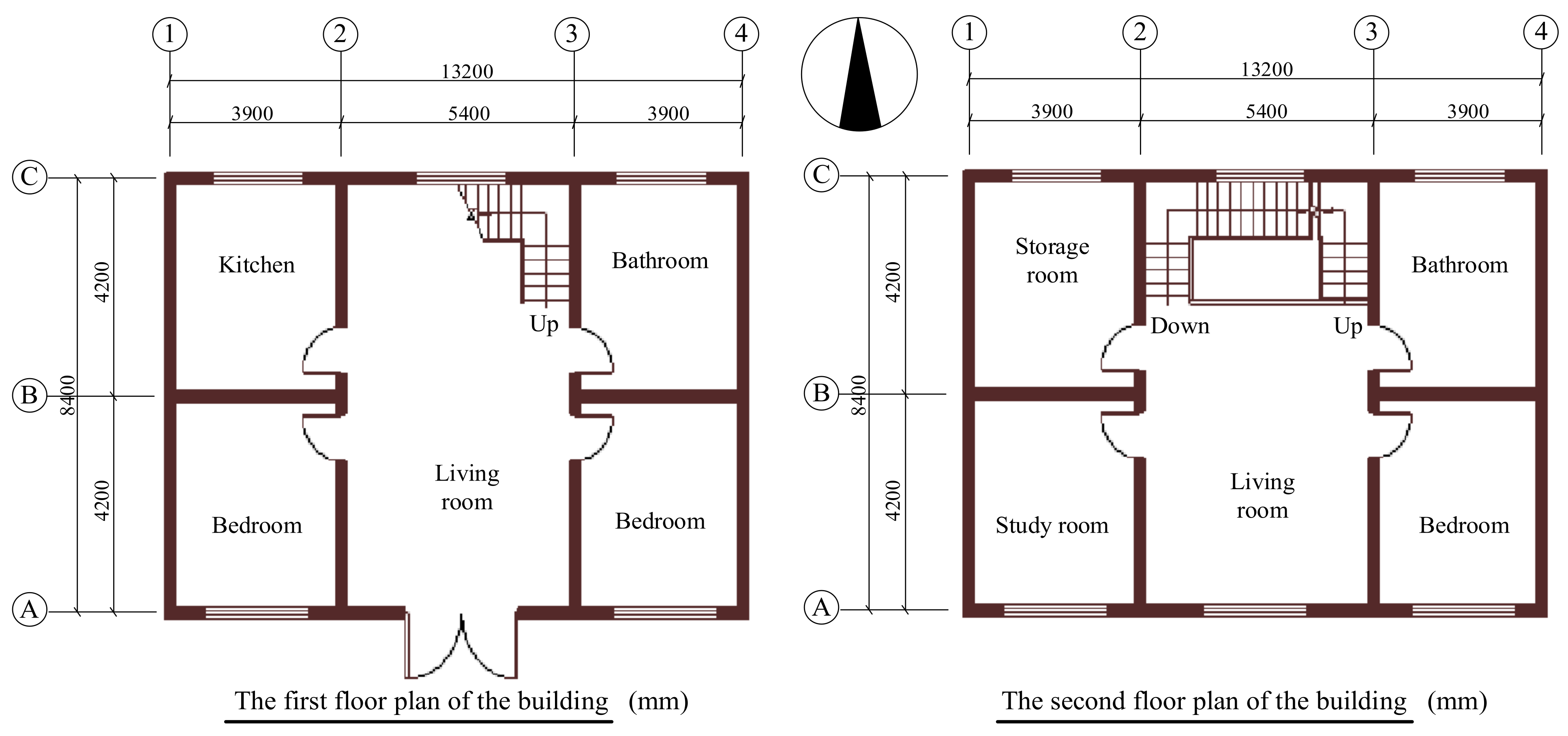
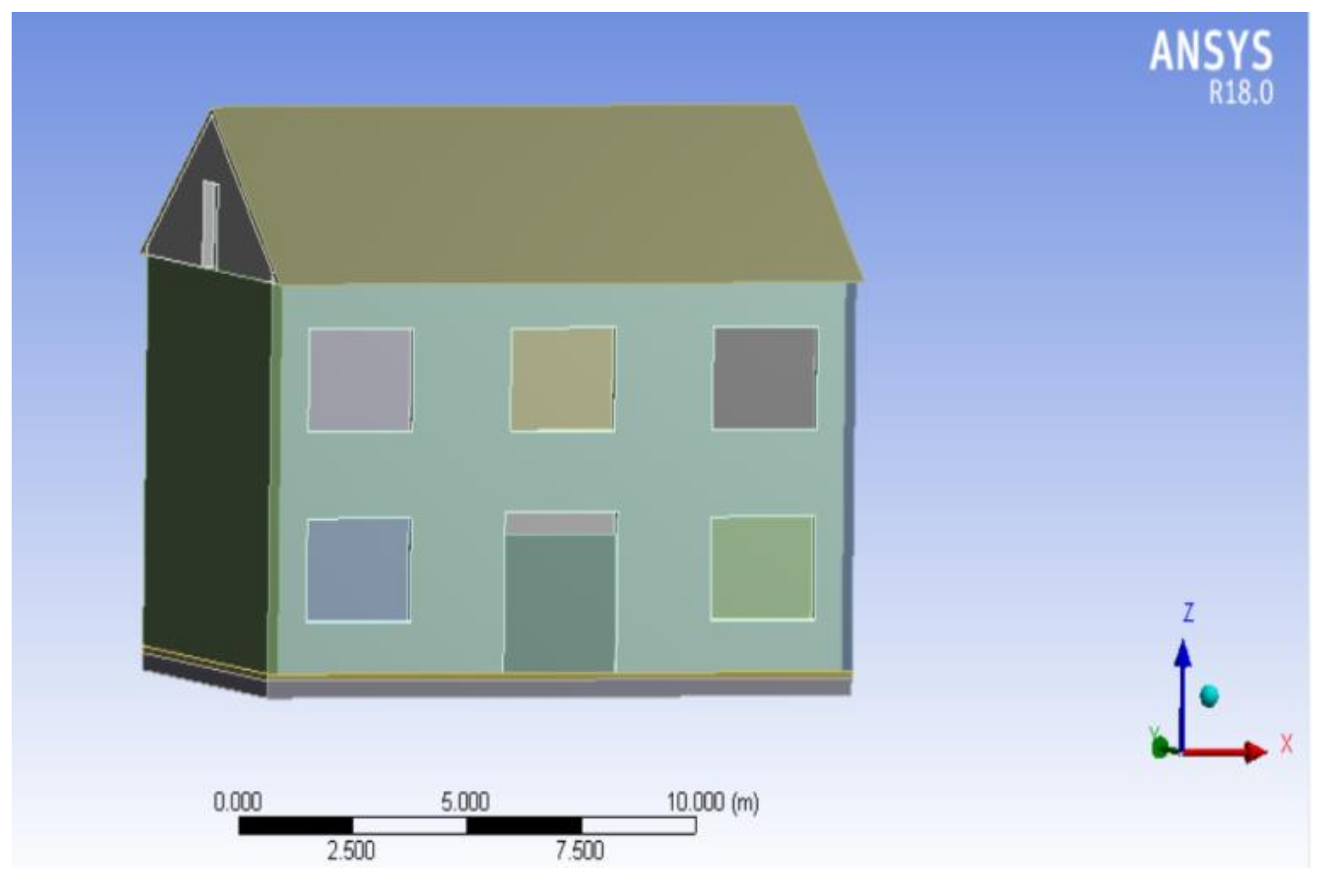
- 1.
- Basic assumptions and geometric modelsTo simplify the model calculation, the following assumptions were used before modeling:
- (1)
- The air in each indoor room is considered as a whole. Its heat transfer mode is natural convection heat transfer.
- (2)
- The indoor door is open. The door is half-open.
- (3)
- The influence of indoor human activities and electrical appliances on the indoor temperature is ignored.
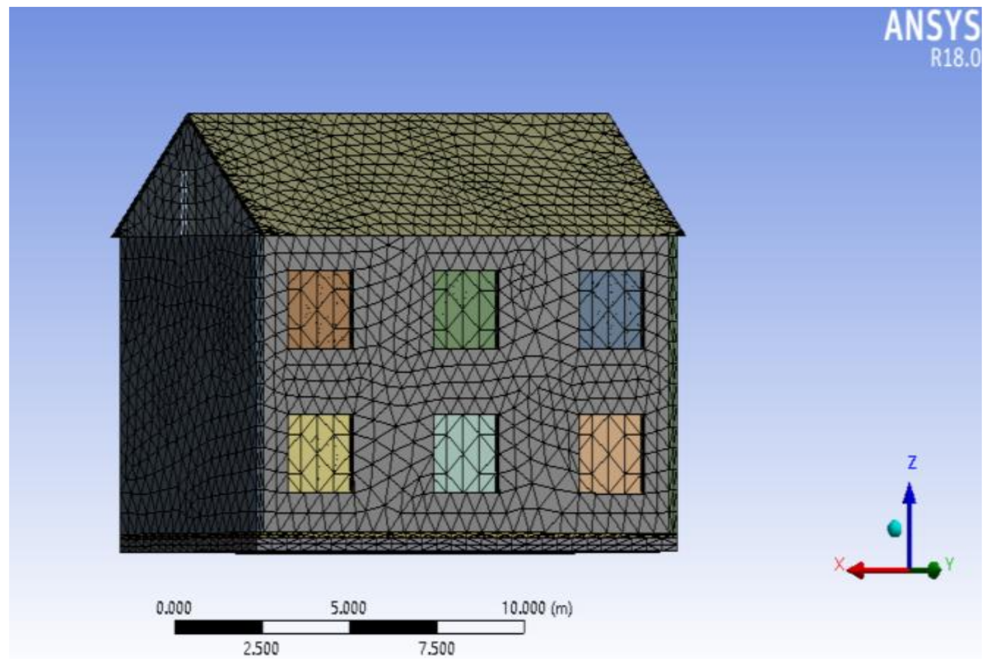
- 2.
- Mesh division
- 3.
- Material parameter setting
- 4.
- Boundary condition setting
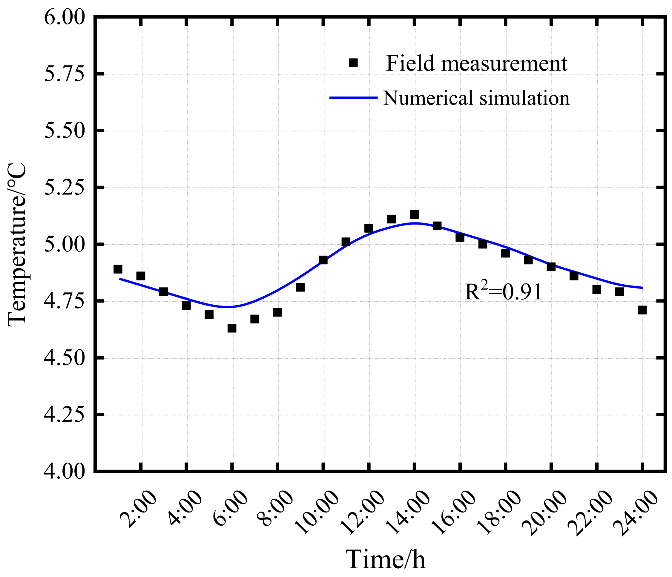
- 5.
- Validation of the model
3. Results and Analysis
3.1. Analysis of Thermal and Mechanical Performances of AASCCIBs
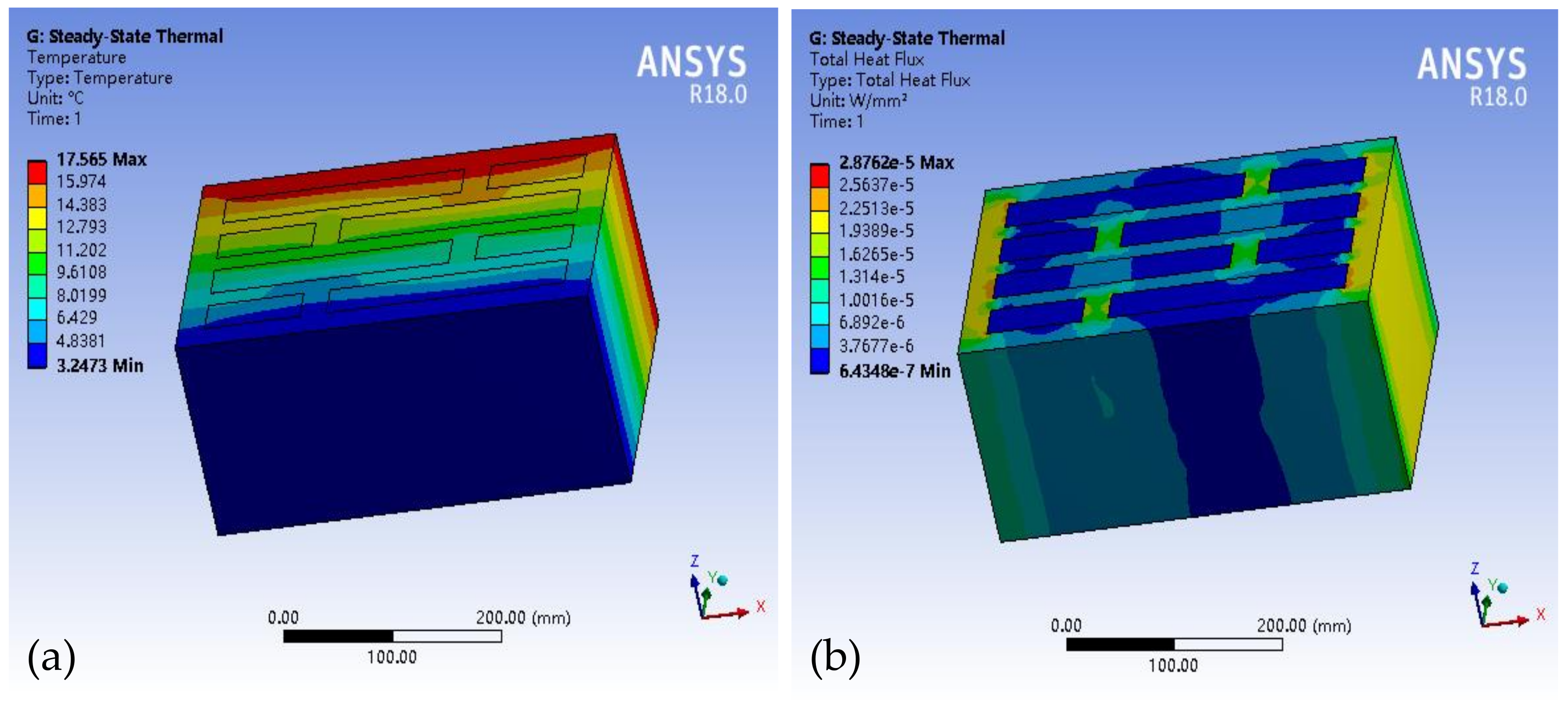
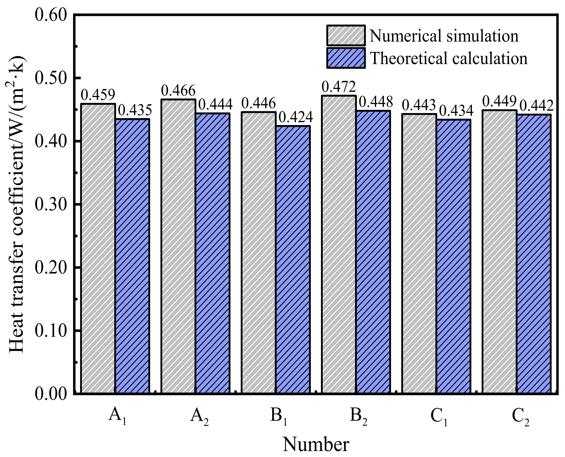
3.1.1. Thermal Performances
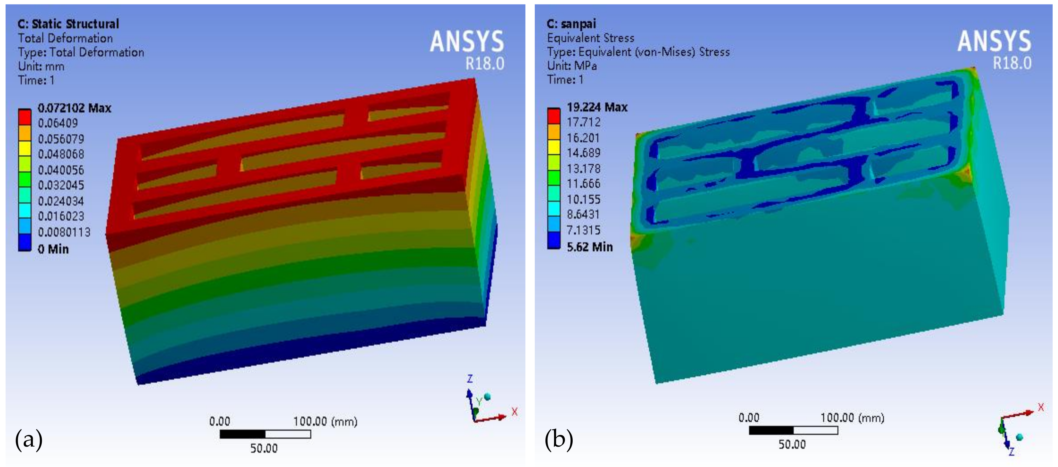
3.1.2. Mechanical Performances
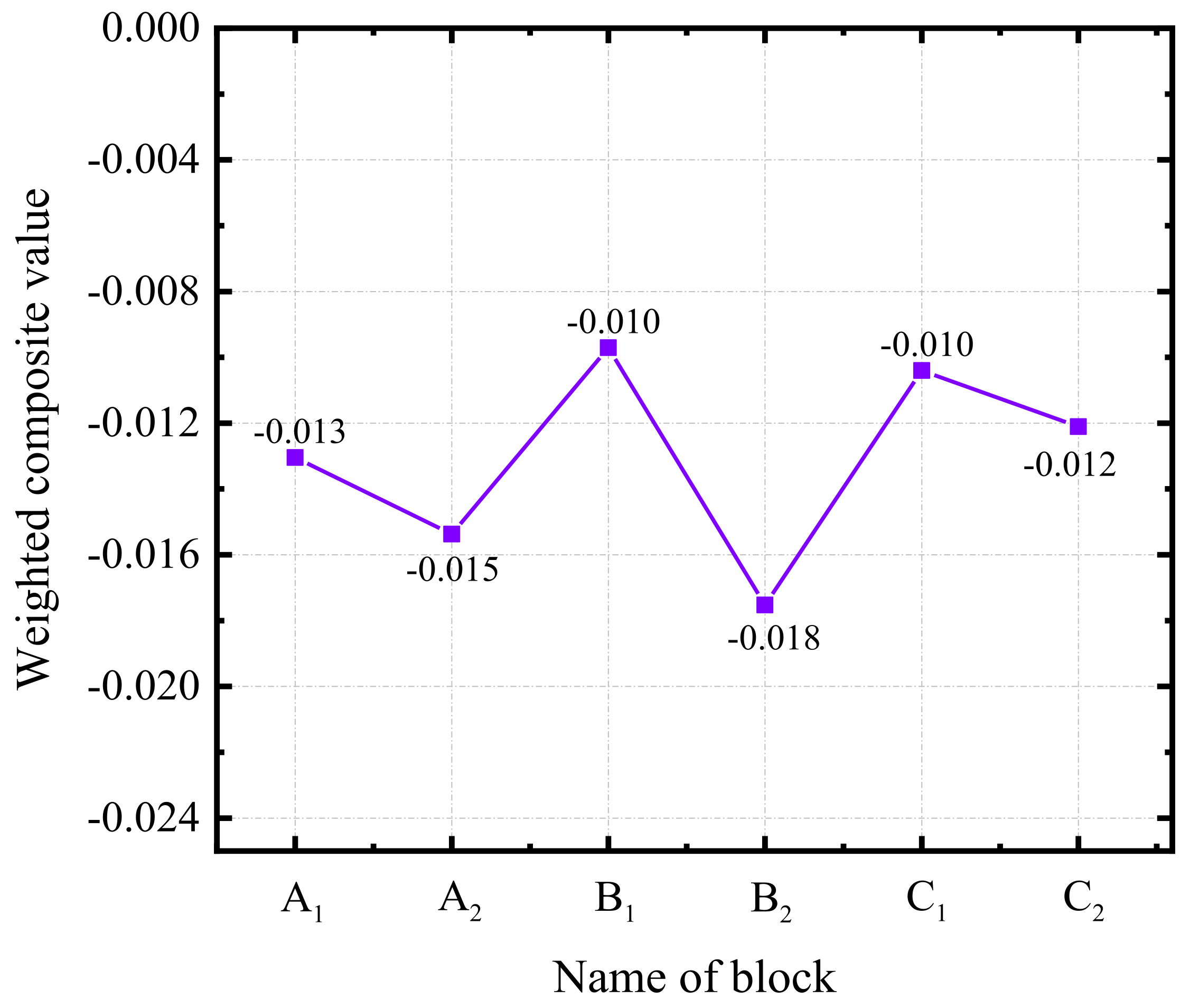
3.2. Determination of Optimal AASCCIBs
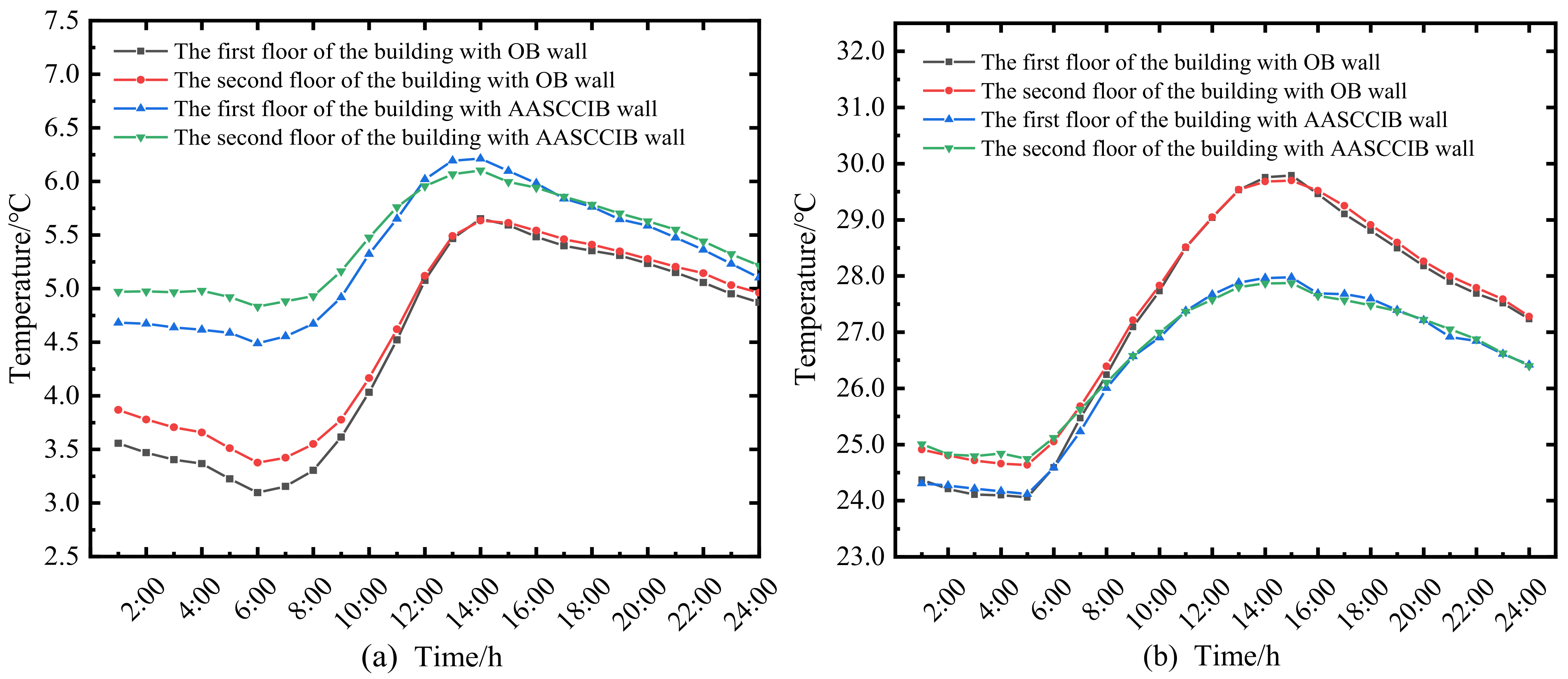
3.3. Improvement Effect of AASCCIB Wall on the Indoor Thermal Environment
4. Conclusions and Outlook
- 1.
- The von Mises equivalent stress and heat transfer coefficient of the AASCCIB decreased with the increase in hole ratio when the hole shape and number of hole rows were constant.
- 2.
- had the optimal comprehensive performance among the six AASCCIBs. The heat transfer coefficient and average von Mises equivalent stress of were 0.446 W/(m2∙K) and 9.52 MPa, respectively.
- 3.
- Compared with the indoor lowest and average temperatures of the building with the OB wall, those of the building with the AASCCIB wall increased by at least 1.39 and 0.82 °C on the winter solstice, respectively. The indoor temperature difference decreased by at least 0.83 °C. In addition, the indoor highest temperature, average temperature, and temperature difference decreased by at least 1.75, 0.79, and 1.89 °C on the summer solstice, respectively.
Author Contributions
Funding
Institutional Review Board Statement
Informed Consent Statement
Data Availability Statement
Conflicts of Interest
References
- Li, Y.; He, J. Evaluating the improvement effect of low-energy strategies on the summer indoor thermal environment and cooling energy consumption in a library building: A case study in a hot-humid and less-windy city of China. In Building Simulation; Tsinghua University Press: Beijing, China, 2021; Volume 14, pp. 1423–1437. [Google Scholar]
- Ujanová, P.; Rychtáriková, M.; Mayor, T.S.; Hyder, A. A Healthy, Energy-Efficient and Comfortable Indoor Environment, a Review. Energies 2019, 12, 1414. [Google Scholar] [CrossRef] [Green Version]
- Ahn, J. Improvement of the Performance Balance between Thermal Comfort and Energy Use for a Building Space in the Mid-Spring Season. Sustainability 2020, 12, 9667. [Google Scholar] [CrossRef]
- Zhu, Y.Y.; Fan, X.N.; Wang, C.J.; Sang, G.C. Analysis of Heat Transfer and Thermal Environment in a Rural Residential Building for Addressing Energy Poverty. Appl. Sci. 2018, 8, 2077. [Google Scholar] [CrossRef] [Green Version]
- Kalua, A. Urban Residential Building Energy Consumption by End-Use in Malawi. Buildings 2020, 10, 31. [Google Scholar] [CrossRef] [Green Version]
- Xu, X.; Mumford, T.; Zou, P. Life-cycle building information modelling (BIM) engaged framework for improving building energy performance. Energy Build. 2020, 231, 110496. [Google Scholar] [CrossRef]
- Alsheyab, M. Recycling of construction and demolition waste and its impact on climate change and sustainable development. Int. J. Environ. Sci. Technol. 2021, 1, 1–10. [Google Scholar]
- Liu, H.W.; Li, J.; Su, Y.F.; Wang, Y.S. Estimation Method of Carbon Emissions in the Embodied Phase of Low Carbon Building. Adv. Civ. Eng. 2020, 2020, 8853536. [Google Scholar]
- Li, R.Y.; Li, Y.Y. Discussion on the innovation of new wall materials. Charming China 2014, 22, 263. [Google Scholar]
- Li, P.; Sun, D.S.; Ding, Y.; Wang, A.G. Thermal Testing and Simulation of Self-thermal Insulation Block. China Concr. Cem. Pro. 2015, 8, 63–66. [Google Scholar]
- Jiao, Z.; Wang, Y.; Zheng, W.; Huang, W.; Zhou, X. Use of Industrial Waste Slag in Alkali-Activated Slag Ceramsite Concrete Hollow Blocks. Appl. Sci. 2018, 8, 2358. [Google Scholar] [CrossRef] [Green Version]
- Rashad, A.M. Recycled waste glass as fine aggregate replacement in cementitious materials based on Portland cement. Constr. Build. Mater. 2014, 72, 340–357. [Google Scholar] [CrossRef]
- Imbabi, M.; Carrigan, C.; Mckenna, S. Trends and developments in green cement and concrete technology. Int. J. Sustain. Built Environ. 2012, 1, 194–216. [Google Scholar] [CrossRef] [Green Version]
- Awoyera, P.; Adesina, A. A critical review on application of alkali activated slag as a sustainable composite binder. Case Studies Constr. Mater. 2019, 11, e00268. [Google Scholar] [CrossRef]
- Rodríguez, E.D.; Mejia, R.; Puertas, F. Alternative concrete based on alkali-activated slag. Mater. Constr. 2008, 58, 53–67. [Google Scholar]
- Liu, S.X.; Shen, L.L.; Niu, F.S. Researching Status and Prospect of Lightweight Aggregates Obtained from Solid Wastes in China. Adv. Mater. Res. 2011, 163–167, 624–628. [Google Scholar] [CrossRef]
- Xie, J.; Liu, J.; Liu, F.; Wang, J.; Huang, P. Investigation of a new lightweight green concrete containing sludge ceramsite and recycled fine aggregates. J. Clean. Prod. 2019, 235, 1240–1254. [Google Scholar] [CrossRef]
- Li, M.; Zhou, D.Y.; Jiang, Y.Q. Preparation and Thermal Storage Performance of Phase Change Ceramsite Sand and Thermal Storage Light-weight Concrete. Renew. Energy 2021, 175, 143–152. [Google Scholar] [CrossRef]
- Sang, G.C.; Du, X.Y.; Zhang, Y.K.; Zhao, C.Y.; Cui, X.L.; Cui, H.Z.; Zhang, L.; Zhu, Y.Y.; Guo, T. A novel composite for thermal energy storage from alumina hollow sphere/paraffin and alkali-activated slag. Ceram. Int. 2021, 47, 15947. [Google Scholar] [CrossRef]
- Akgul, B.A.; Karapınar, E. Investigation and Evaluation of Thermal Analysis for Different Wall Structures with Finite Element Method, Simulation of Temperature Distribution and Reaction in the Wall Types. Euro. J. Math. Eng. Nat. Med. Sci. 2021, 8, 132–144. [Google Scholar]
- Ait-Taleb, T.; Abdelbaki, A.; Zrikem, Z. Simulation of coupled heat transfers in a hollow tile with two vertical and three horizontal uniform rectangular cavities heated from below or above. Energy Build. 2014, 84, 628–632. [Google Scholar] [CrossRef]
- Boukendil, M.; Abdelbaki, A.; Zrikem, Z. Simulation of the temperature field for massive concrete structures using an interval finite element method. Eng. Comput. 2020, 37, 2467–2486. [Google Scholar]
- Hawkes, P.W.; Kasper, E. 11-The Finite-Difference Method (FDM). Principl. Electr. Opt. 1996, 116, 159–174. [Google Scholar]
- Mazumder, S. The Finite Difference Method—ScienceDirect. Numer. Methods Partial Differ. Equ. 2016, 12, 51–101. [Google Scholar]
- Cheng, Y.M.; Bai, F.N.; Peng, M.J. A novel interpolating element-free Galerkin (IEFG) method for two-dimensional elastoplasticity. Appl. Math. Model. 2014, 38, 5187–5197. [Google Scholar] [CrossRef]
- Mukherjee, S.; Liu, Y. The Boundary Element Method. Int. J. Comp. Meth-Sing. 2013, 10, 1350037. [Google Scholar] [CrossRef]
- Mazumder, S. The Finite Volume Method (FVM). Numer. Meth. Part. Differ. Equ. 2016, 1, 277–338. [Google Scholar]
- Teng, C.; Yang, Q.; Peng, H. Numerical Thermal Optimization of the Hole Structures of Pottery Grain Concrete Hollow Blocks. Mater. Rev. 2011, 25, 280–284. [Google Scholar]
- Gao, H.; Wei, G. Complex Variable Meshless Manifold Method for Transient Heat Conduction Problems. Int. J. Appl. Mech. 2017, 9, 1750067. [Google Scholar] [CrossRef]
- Gao, H.; Wei, G. Numerical solution of Potential Problems using Radial Basis Reproducing Kernel Particle Method. Results Phys. 2019, 13, 102122. [Google Scholar] [CrossRef]
- Muttalli, R.S.; Agrawal, S.; Warudkar, H. CFD Simulation of Centrifugal Pump Impeller Using ANSYS-CFX. Int. J. Innov. Res. Sci. Eng. Technol. 2014, 3, 15553–15561. [Google Scholar] [CrossRef]
- MOHURD. Self-Insulation Concrete Compound Blocks: JG/T 407-2013; China Architecture Building Press: Beijing, China, 2013. [Google Scholar]
- Zheng, J.S.; Zhang, G.Z. Design and heat transfer performance of warming compound blocks with slag concrete. New Build. Mater. 2012, 39, 63–65. [Google Scholar]
- Bathe, K.J. Finite Element Procedures; Prentice-Hall: Hoboken, NJ, USA, 2006. [Google Scholar]
- Sardari, P.T.; Mohammed, H.I.; Mahdi, J.M.; Ghalambaz, M.; Gillott, M.; Walker, G.S.; Grant, D.; Giddings, D. Localized heating element distribution in composite metal foam-phase change material: Fourier’s law and creeping flow effects. Int. J. Energy Res. 2021, 45, 13380–13396. [Google Scholar] [CrossRef]
- Arif, M.; Kaushik, S.K. Convexity studies of two anisotropic yield criteria in principal stress space. Eng. Comput. 1999, 16, 215–229. [Google Scholar]
- Li, Q.; Steven, G.P.; Xie, Y.M. On equivalence between stress criterion and stiffness criterion in evolutionary structural optimization. Struct. Optim. 1999, 18, 67–73. [Google Scholar] [CrossRef]
- Pazera, E. Heat Transfer in Periodically Laminated Structures-Third Type Boundary Conditions. Int. J. Comput. Meth. 2021, 18, 2041011. [Google Scholar] [CrossRef]
- MOHURD. Code for Thermal Design of Civil Building: CB50176-2016; China Architecture Building Press: Beijing, China, 2016. [Google Scholar]
- MOHURD. Design Standard for Energy Efficiency of Rural Residential Buildings: GB50176-2016; China Architecture Building Press: Beijing, China, 2016. [Google Scholar]
- MOHURD. Design Standards for Energy Efficiency of Residential Buildings in Hot Summer and Cold Winter Zones: JGJ134-2010; China Architecture Building Press: Beijing, China, 2010. [Google Scholar]
- Sánchez-Zarco, X.G.; González-Bravo, R.; Ponce-Ortega, J.M. Multi-objective Optimization Approach to Meet Water, Energy, and Food Needs in an Arid Region Involving Security Assessment. ACS Sustain. Chem. Eng. 2021, 9, 4771–4790. [Google Scholar] [CrossRef]
- Hamka, M.; Harjono, H. Application of fuzzy preference relations method in AHP to improve judgment matrix consistency. In IOP Conference Series: Materials Science and Engineering; IOP Publishing: Bristol, UK, 2020; Volume 821, p. 12035. [Google Scholar]
- Yang, Z.T.; Liu, Y.; Yin, G.S.; Shi, M.H.; Wei, P.F. Optimization design and analysis of multi-row ceramsite concrete composite block structure. Bull. Chin. Ceram. Soc. 2020, 39, 113–123. [Google Scholar]
- Zhao, Q.; Fan, X.N.; Wang, Q.; Sang, G.C.; Zhu, Y.Y. Research on Energy-Saving Design of Rural Building Wall in Qinba Mountains Based on Uniform Radiation Field. Math. Probl. Eng. 2020, 2020, 9786895. [Google Scholar] [CrossRef]
- Chandrupatla, T.R.; Belegundu, A.D. Introduction to Finite Element in Engineering; Prentice-Hall: Hoboken, NJ, USA, 1991. [Google Scholar]
- Zhang, Q.Y.; Huang, J. Standard Meteorological Database Used for Buildings in China; Mechanical Industry Press: Beijing, China, 2004. [Google Scholar]
- Samoshkin, S.L.; Meyster, A.O.; Yukhnevskiy, M.A. Methodical issues of determination of the average heat transfer coefficient of the passenger car body. Vest. Rail. Res. Ins. 2020, 78, 344–350. [Google Scholar] [CrossRef] [Green Version]
- Guo, T.M.; Hu, S.T.; Liu, G.D. Evaluation Model of Specific Indoor Environment Overall Comfort Based on Effective-Function Method. Energies 2017, 10, 1634. [Google Scholar] [CrossRef]


| Number | Number of Hole Rows | a | b | c | d | e | f | Hole Ratio/% |
|---|---|---|---|---|---|---|---|---|
| Three rows | 25 | 225 | 25 | 90 | 44 | 29 | 44.4 | |
| 25 | 225 | 25 | 90 | 42 | 32 | 42.4 | ||
| Four rows | 25 | 225 | 25 | 90 | 34 | 18 | 45.8 | |
| 25 | 225 | 25 | 90 | 31 | 22 | 41.7 | ||
| Five rows | 25 | 225 | 25 | 90 | 26 | 15 | 43.8 | |
| 25 | 225 | 25 | 90 | 25.2 | 16 | 42.9 |
| Note | Thermal Conductivity W/(m∙K) | Density kg/m3 | Specific Heat Capacity J/(kg∙K) | Elastic Modulus MPa | Poisson’s Ratio |
|---|---|---|---|---|---|
| Shell of AASCSIHB | 0.35 | 1600 | 1.05 | 27920 | 0.2 |
| XPS | 0.03 | 35 | 1.38 | / | / |
| Comparison of the Importance of Factor i and Factor j | Scale (aij) |
|---|---|
| i and j are equally important | 1 |
 | 3 |
| 5 | |
| 7 | |
| 9 | |
| The median value of two adjacent scales | 2, 4, 6, 8 |
| Item | Material Layer | Thickness mm | Thermal Conductivity W/(m∙K) | Density Kg/m3 | Specific Heat Capacity J/(kg∙K) |
|---|---|---|---|---|---|
| External wall (OB wall) | Cement mortar | 20 | 0.93 | 1800 | 1050 |
| Solid clay brick | 240 | 0.81 | 1800 | 1050 | |
| Cement mortar | 20 | 0.93 | 1800 | 1050 | |
| External wall (AASCCIB wall) | Cement mortar | 20 | 0.93 | 1800 | 1050 |
| AASCCIB | 240 | 0.11 | 867 | 1050 | |
| Cement mortar | 20 | 0.93 | 1800 | 1050 | |
| Partition wall | Cement mortar | 20 | 0.93 | 1800 | 1050 |
| Solid clay brick | 240 | 0.81 | 1800 | 1050 | |
| Cement mortar | 20 | 0.93 | 1800 | 1050 | |
| Floor | Cement mortar | 20 | 0.93 | 1800 | 1050 |
| Reinforced concrete | 100 | 1.74 | 2500 | 920 | |
| Cement mortar | 20 | 0.93 | 1800 | 1050 | |
| Roof | Clay tile | 20 | 1.00 | 2000 | 800 |
| Wooden rafter | 100 | 0.17 | 650 | 2120 | |
| Ground | Pebble concrete | 100 | 1.51 | 2300 | 920 |
| Compacted clay | 300 | 1.16 | 2000 | 1010 | |
| Window | Single-layer clear glass | 3 | 0.76 | 2500 | 840 |
| Door | Wood | 150 | 0.35 | 500 | 2510 |
| Number | Number of Hole Rows | Hole Ratio % | Temperature Difference °C | Heat Flux Intensity W/m2 | Heat Transfer Coefficient W/(m2·K) |
|---|---|---|---|---|---|
| Three rows | 44.4 | 13.871 | 6.360 | 0.459 | |
| 42.4 | 13.848 | 6.452 | 0.466 | ||
| Four rows | 45.8 | 13.881 | 6.185 | 0.446 | |
| 41.7 | 13.841 | 6.531 | 0.472 | ||
| Five rows | 43.8 | 13.885 | 6.163 | 0.444 | |
| 42.9 | 13.871 | 6.225 | 0.449 |
| Number | Number of Hole Rows | Hole Ratio % | Maximum von Mises Equivalent Stress/MPa | Minimum von Mises Equivalent Stress/MPa | Average von Mises Equivalent Stress/MPa |
|---|---|---|---|---|---|
| Three rows | 44.4 | 19.22 | 5.62 | 9.553 | |
| 42.4 | 18.70 | 5.59 | 9.559 | ||
| Four rows | 45.8 | 18.81 | 5.73 | 9.517 | |
| 41.7 | 19.27 | 5.64 | 9.524 | ||
| Five rows | 43.8 | 18.80 | 5.67 | 9.496 | |
| 42.9 | 18.78 | 5.67 | 9.502 |
| Number | Number of Hole Rows | Heat Transfer Coefficient | Equivalent Stress | Hole Ratio |
|---|---|---|---|---|
| Three rows | 0.168 | 0.1671 | 0.170 | |
| 0.170 | 0.1673 | 0.162 | ||
| Four rows | 0.163 | 0.1665 | 0.175 | |
| 0.173 | 0.1666 | 0.160 | ||
| Five rows | 0.162 | 0.1662 | 0.168 | |
| 0.164 | 0.1663 | 0.164 |
Publisher’s Note: MDPI stays neutral with regard to jurisdictional claims in published maps and institutional affiliations. |
© 2021 by the authors. Licensee MDPI, Basel, Switzerland. This article is an open access article distributed under the terms and conditions of the Creative Commons Attribution (CC BY) license (https://creativecommons.org/licenses/by/4.0/).
Share and Cite
Fan, X.; Guo, Y.; Zhao, Q.; Zhu, Y. Structural Optimization and Application Research of Alkali-Activated Slag Ceramsite Compound Insulation Block Based on Finite Element Method. Mathematics 2021, 9, 2488. https://doi.org/10.3390/math9192488
Fan X, Guo Y, Zhao Q, Zhu Y. Structural Optimization and Application Research of Alkali-Activated Slag Ceramsite Compound Insulation Block Based on Finite Element Method. Mathematics. 2021; 9(19):2488. https://doi.org/10.3390/math9192488
Chicago/Turabian StyleFan, Xiaona, Yu Guo, Qin Zhao, and Yiyun Zhu. 2021. "Structural Optimization and Application Research of Alkali-Activated Slag Ceramsite Compound Insulation Block Based on Finite Element Method" Mathematics 9, no. 19: 2488. https://doi.org/10.3390/math9192488
APA StyleFan, X., Guo, Y., Zhao, Q., & Zhu, Y. (2021). Structural Optimization and Application Research of Alkali-Activated Slag Ceramsite Compound Insulation Block Based on Finite Element Method. Mathematics, 9(19), 2488. https://doi.org/10.3390/math9192488