Article

A Dimension Splitting Generalized Interpolating Element-Free Galerkin Method for the Singularly Perturbed Steady Convection–Diffusion–Reaction Problems

1
Faculty of Science, Ningbo University of Technology, Ningbo 315016, China
2
College of Finance & Information, Ningbo University of Finance & Economics, Ningbo 315175, China
3
Faculty of Maritime and Transportation, Ningbo University, Ningbo 315211, China
*
Author to whom correspondence should be addressed.
Mathematics 2021, 9(19), 2524; https://doi.org/10.3390/math9192524
Submission received: 26 August 2021 / Revised: 3 October 2021 / Accepted: 5 October 2021 / Published: 8 October 2021

Abstract

:
By introducing the dimension splitting method (DSM) into the generalized element-free Galerkin (GEFG) method, a dimension splitting generalized interpolating element-free Galerkin (DS-GIEFG) method is presented for analyzing the numerical solutions of the singularly perturbed steady convection–diffusion–reaction (CDR) problems. In the DS-GIEFG method, the DSM is used to divide the two-dimensional CDR problem into a series of lower-dimensional problems. The GEFG and the improved interpolated moving least squares (IIMLS) methods are used to obtain the discrete equations on the subdivision plane. Finally, the IIMLS method is applied to assemble the discrete equations of the entire problem. Some examples are solved to verify the effectiveness of the DS-GIEFG method. The numerical results show that the numerical solution converges to the analytical solution with the decrease in node spacing, and the DS-GIEFG method has high computational efficiency and accuracy.

1. Introduction

Since the construction of the approximation function is independent of the mesh, the meshless method, which has developed rapidly in recent years, can completely abandon the mesh reconstruction to ensure high calculation accuracy [1,2,3]. The meshless method has become an essential numerical method in scientific and engineering computation [4,5,6,7].
When studying surface fitting, Lancaster and Salkauskas proposed the moving least squares (MLS) approximation [8], which is based on the traditional least squares (LS) method [9,10,11,12]. The MLS is one of the most important methods for constructing trial functions in meshless methods [13]. Based on the MLS approximation, Belytschko et al. proposed the element-free Galerkin (EFG) method [14], which has a wide range of applications and high calculation accuracy. Since the shape function of the MLS approximation does not satisfy the Kronecker delta property [15], additional numerical techniques are required to impose essential boundary conditions, such as Lagrange multipliers, a penalty method, which may increase the computational burden. For this reason, Lancaster et al. proposed the interpolated moving least-squares (IMLS) method [8] by selecting singular special weight functions. Since the singularity of the weight function is not conducive to numerical calculation, Cheng et al. proposed an improved interpolated moving least squares (IIMLS) method with nonsingular weights for potential problems [16]. The improved meshless method based on the IIMLS has the advantages of nonsingular weight function and direct application of an essential boundary [17,18].
Many meshless methods have been presented [19], such as the smooth particle hydrodynamics method, element-free Galerkin (EFG) method, reproducing kernel particle method, hp-cloud method, and meshless local Petrov–Galerkin (MLPG) method. Peridynamics (PD) is also an important meshless method for solving solid and fluid mechanics problems [20,21]. When the EFG method is used to solve some fluid problems, the numerical solution is prone to non-physical oscillation [22,23,24]. By coupling the variational multiscale method and EFG method, Ouyang et al. established the variational multiscale EFG method (VMEFG) [25]. The VMEFG method has been successfully applied in many physical problems [26,27,28]. However, the disadvantage of VMEFG is that the bubble function in the stabilization factor must be based on the mesh and is difficult to construct in high-dimensional cases. Li et al. proposed the general element-free Garlerkin (GEFG) method [22] for Stokes problems. The GEFG method overcomes the non-physical oscillation of the solution caused by the EFG method, and also overcomes the deficiency that the stabilization factor of the VMEFG method must be related to the mesh.
Due to the complexity of the shape function, the traditional EFG method requires a large amount of calculation, especially for three-dimensional problems. Then, Cheng et al. proposed the dimension-splitting element-free Galerkin method by coupling the dimension-splitting method (DSM) and EFG method [29,30,31]. Since the DSM divides high-dimensional problems into a series of low-dimensional problems and then iteratively solves them, it can effectively improve the computational efficiency of numerical methods [32,33]. Therefore, the dimension-splitting element-free Galerkin method can significantly improve the computational efficiency of the EFG method [34].
The convection–diffusion–reaction (CDR) equation has a wide range of applications in the fields of physics and chemistry [35,36,37]. The steady CDR equation can model the transport of the quantity and represent the balance of three processes: transport by convection, diffusion and reactions [37]. As it is difficult to obtain the analytical solutions of the CDR equation in complex situations, many numerical methods have been proposed to obtain the numerical solutions [38,39,40]. A finite difference method [36] and two spurious oscillations at layers diminishing (SOLD) methods [37] have been presented for solving steady CDR problems. For the singularly perturbed problems, the numerical solutions are prone to instability issues [41,42]. Then, when the diffusion coefficient is very small in CDR problems, it is usually necessary to add additional stability measures to ensure that the numerical method obtains a stable solution [43]. Wu et al. presented an adaptive upwind finite difference method for the CDR problem with two small parameters [44]. The finite difference method [45], a cubic B-spline-based semi-analytical algorithm [46], and weak Galerkin method [47] are proposed for studying the numerical solutions of the CDR problems.
Due to the advantages of the meshless method, some meshless methods have been developed for the CDR problems [48,49]. Zhang and Xiang discussed the numerical solutions of the CDR equation with small diffusion by the VMEFG method [50,51]. Li et al. also applied the local Petrov Galerkin method to the multi-dimensional CDR equations based on the radial basis function [52]. Additionally, the local knot method [53] and the meshless boundary collocation method [54] have been presented to solve the numerical solution of the CDR equation.
In this paper, by constructing the trial functions from the IIMLS method and coupling the DSM and GEFG method, a dimension splitting general interpolating element-free Galerkin (DS-GIEFG) method is presented for the singularly perturbed steady CDR problems. In the DS-GIEFG method, DSM divides the two-dimensional problem into a series of one-dimensional problems. The GEFG method is used to establish the discrete equations on the low-dimensional problems. Finally, the IIMLS method is used to assemble the discrete equations on the entire problem domain. The DS-GIEFG method will have high computational efficiency and solution stability for the singularly perturbed steady CDR problem.

2. The DS-GIEFG Method for CDR Problems

By using the interpolating shape function of the IIMLS method and coupling the DSM and GEFG method, we will present the DS-GIEFG method for the singularly perturbed steady CDR problems.

2.1. The Trial Functions for the DS-GIEFG Method

The trial function of the DS-GIEFG method is presented by using the property of the PU function. From the Refs. [14,16], the following properties are satisfied:
i = 1 n Φ i ( y ) b ( y i ) = b ( y )
where y i is the discrete node, Φ i and b are, respectively, the shape functions and the basis functions used in the IIMLS method [16].
Then, if the basis functions are chosen to be the complete polynomials of order m , the PU function can be established as follows [16]
i = 1 n Φ i = 1
Similar to the GEFG method [22], the trial function of the DS-GIEFG method is defined as
u h ( y ) = i = 1 n Φ i ( y ) τ i ( y )
where the function τ k ( y ) is
τ i ( y ) = j = 1 m i θ i j ( y ) c i j
Here, the function θ i j ( y ) and c i j are, respectively, the nodal enrichment basis function and the corresponding coefficient to be determined of y i , and m i is the number of the local enrichment basis function. The purpose of introducing local enrichment polynomial basis functions is to increase the stability of the meshless method to fluid problems. When m i = 1, the trial function (3) is consistent with that of the EFG method.
According to reference [22,55], we take the local polynomial basis function as the enrichment basis function. In one-dimensional space, θ k j ( y ) can be taken as the following forms [22,55]:
(a)
If m i = 1 , then θ i 1 ( y ) = 1 .
(b)
if m i = 2 , then { θ i 1 ,   θ i 2 } = { 1 ,   ( y y i ) 2 } .
(c)
if m i = 3 , then { θ i 1 ,   θ i 2 ,   θ i 3 } = { 1 ,   ( y y i ) 2 , ( y y i ) 3 } .
For example, when m i = 2, the trial function of the DS-GIEFG method in one-dimensional space is:
u h = i = 1 n Φ i ( y ) c i 1 + i = 1 n Φ i ( y ) ( y y i ) 2 c i 2
In Equation (5), the first term represents the effect of the IIMLS method, and the second term is the stabilization parameter of the DS-GIEFG method for the singularly perturbed steady CDR problems.

2.2. Discretization Process on the Splitting Plane

The following two-dimensional singular perturbed steady CDR equations are considered:
{ a u ε Δ u + c u = f , in   Ω R 2 , u = u D , on   boundary   Γ .
Equation (6) can model the transport of the quantity u = u ( x , y ) . The prescribed function f is the source term describing chemical reactions, and u D is a given functions for the Dirichlet condition. a = ( a 1 , a 2 ) T denotes velocity field, 0 < ε 1 denotes the small diffusion coefficient, and c is the reaction coefficient.
Let L denote the number of the splitting plane. According to the idea of the DSM, the problem (6) is divided into a series of one-dimensional problems on the split surface y :
{ ( a u ε Δ u + c u ) | x = x k = f | x = x k , in   Ω k = Ω { x = x k } , u = u D , on   boundary   Γ ,
where Ω k ( k = 1 , 2 , , L ) is a splitting plane such that
Ω = k = 1 L Ω k × ( x k 1 , x k ]
Define V ( k ) H 1 ( Ω k ) C 0 ( Ω k ) . The weak form of Equation (7) is
( a u ( k ) , v ) + ε ( v y , u y ( k ) ) ε ( v , u x x ( k ) ) + c ( v , u ( k ) ) = ( v , f ( k ) ) ,   v V ( k )
where u ( k ) = u | x = x k , u y ( k ) = u y | x = x k , u x y ( k ) = 2 u x y | x = x k , and other symbols are similarly defined, and the inner product is:
( v , u ) Ω k u v d y
For   Ω ( k ) , define the numerical solution space as
V h = span { Φ i ( y ) θ i j ( y ) , 1 i n , 1 j m i , y Ω ( k ) }
where Φ i ( y ) is obtained by the IIMLS method on the splitting plane.
From Equation (11), the undetermined function u ( k ) is approximated by
u ( k ) i = 1 n j = 1 m i Φ i ( y ) θ i j ( y ) c i j ( k )
where c i j ( k ) are parameters to be determined.
The matrix form of Equation (12) is
u ( k ) = ϖ ( k ) c ( k ) ( x )
where
ϖ ( k ) = ( Φ 1 ( y ) θ 1 ( k ) ( y ) ,   Φ 2 ( y ) θ 2 ( k ) ( y ) ,   ,   Φ n ( y ) θ n ( k ) ( y ) ) T
θ i ( k ) = ( θ i 1 ( y ) , θ i 2 ( y ) , , θ i m i ( y ) )
c ( x ) = ( c 11 ( x ) , c 12 ( x ) , , c 1 m 1 ( x ) , , c n 1 ( x ) , c n 2 ( x ) , , c n m n ( x ) ) T
From Equation (12), the partial derivatives can be obtained as
u y ( k ) i = 1 n j = 1 m i y [ Φ i ( y ) θ i j ( y ) ] c i j ( k )
u x ( k ) i = 1 n j = 1 m i Φ i ( y ) θ i j ( y ) c i j , x ( k )
where c i j , x ( k ) is the partial derivatives concerning x of c i j ( k ) at x = x k .
Then, the discrete Galerkin weak form of Equation (9) is: for u ¯ ( k ) V h , find u ^ ( k ) V h such that
( u ¯ ( k ) , a u ^ ( k ) ) + ε ( u ¯ y ( k ) , u ^ y ( k ) ) ε ( u ¯ ( k ) , u ^ x x ( k ) ) + c ( u ¯ ( k ) , u ^ ( k ) ) = ( u ¯ ( k ) , f ( k ) )
Substituting Equations (12)–(18) into Equation (19), we can obtain the discrete equations:
ε M 0 ( k ) c x x ( k ) + a 1 M 0 ( k ) c x ( k ) + [ ε M 2 ( k ) + c M 0 ( k ) + a 2 M 1 ( k ) ] c ( k ) = F ( k )
where c x x ( k ) = 2 c ( x ) x 2 | x = x k , c x ( k ) = c ( x ) x | x = x k , c ( k ) = c ( x k ) , and
M 2 ( k ) = Ω ( k ) y ϖ ( k ) ( y ϖ ( k ) ) T d y
M 1 ( k ) = Γ ( k ) ϖ ( k ) ( y ϖ ( k ) ) T d y
M 0 ( k ) = Ω ( k ) ϖ ( k ) ( ϖ ( k ) ) T d y
F ( k ) = Ω ( k ) ϖ ( k ) f ( k ) d y

2.3. Assembling the Discrete Equations of the Whole Problem Domain

The discrete equations of all nodes on Ω will be assembled by using the IIMLS method in the x direction. Let
c ( x ) = s ( x ) ϕ s ( x ) c ( x s ) = s ( x ) ϕ s ( x ) c ( s )
where ϕ i ( x ) denotes the shape function obtained by the IIMLS method in the x direction with the nodes x k , k = 1 , 2 , , L , and ( x ) is an index set of nodes satisfying x in its influence domain.
Then, it follows from Equation (25) that
c x ( k ) = s ( x k ) x ϕ s ( x k ) c ( s )
c x x ( k ) = s ( x k ) 2 x 2 ϕ s ( x k ) c ( s )
Substituting Equations (25)–(27) into Equation (20), it follows
{ [ ε M 2 ( k ) + c M 0 ( k ) + a 2 M 1 ( k ) ] c ( k ) + s ( x k ) ( a 1 x ϕ s ( x k ) M 0 ( k ) ε 2 x 2 ϕ s ( x k ) M 0 ( k ) ) c ( s ) = F ( k ) k = 1 ,   2 ,   ,   L .
On the boundary, the coefficient c i j ( k ) of enrichment basis function will be supposed to be zero. Then, using the interpolation characteristics of the IIMLS method, and substituting the essential boundary conditions into Equation (28), we can solve the coefficients of all nodes in whole Ω . Additionally, then for ( x , y ) Ω , the numerical solution of u is
u h ( x , y ) = s ( x ) i = 1 n j = 1 m i ϕ s ( x ) Φ i ( y ) θ i j ( y ) c i j ( s )

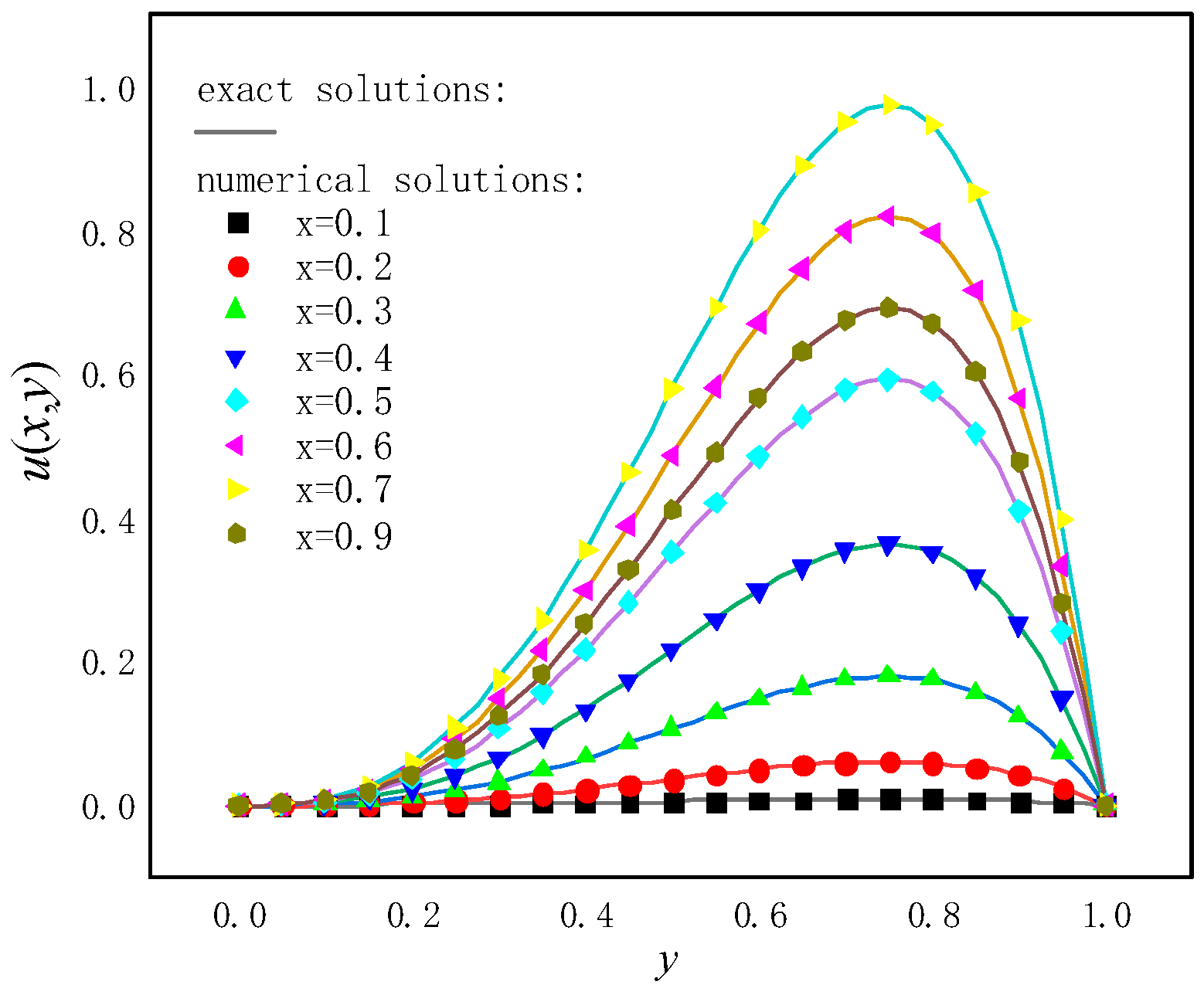
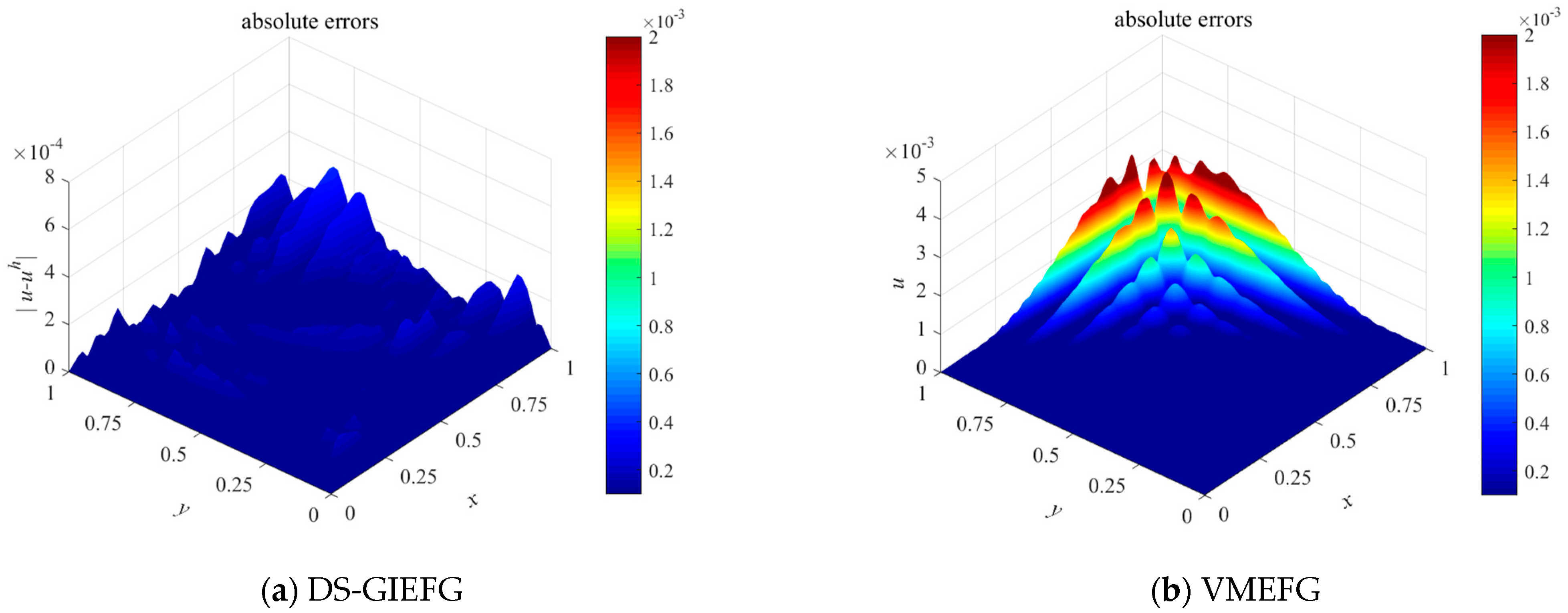
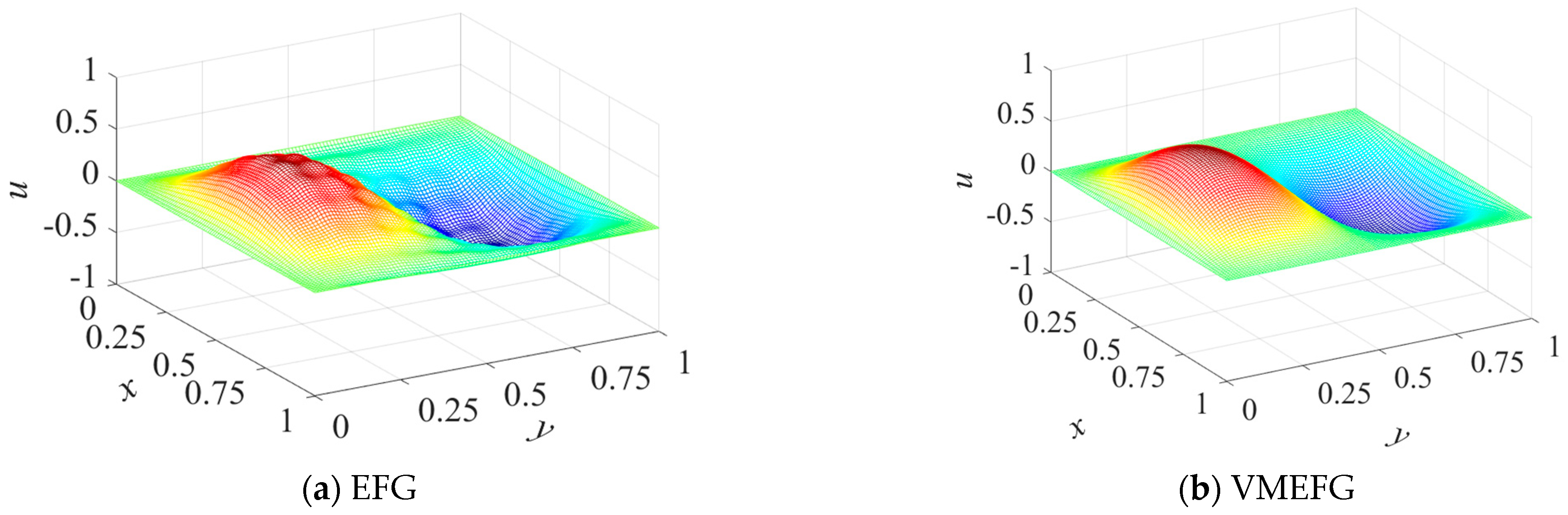
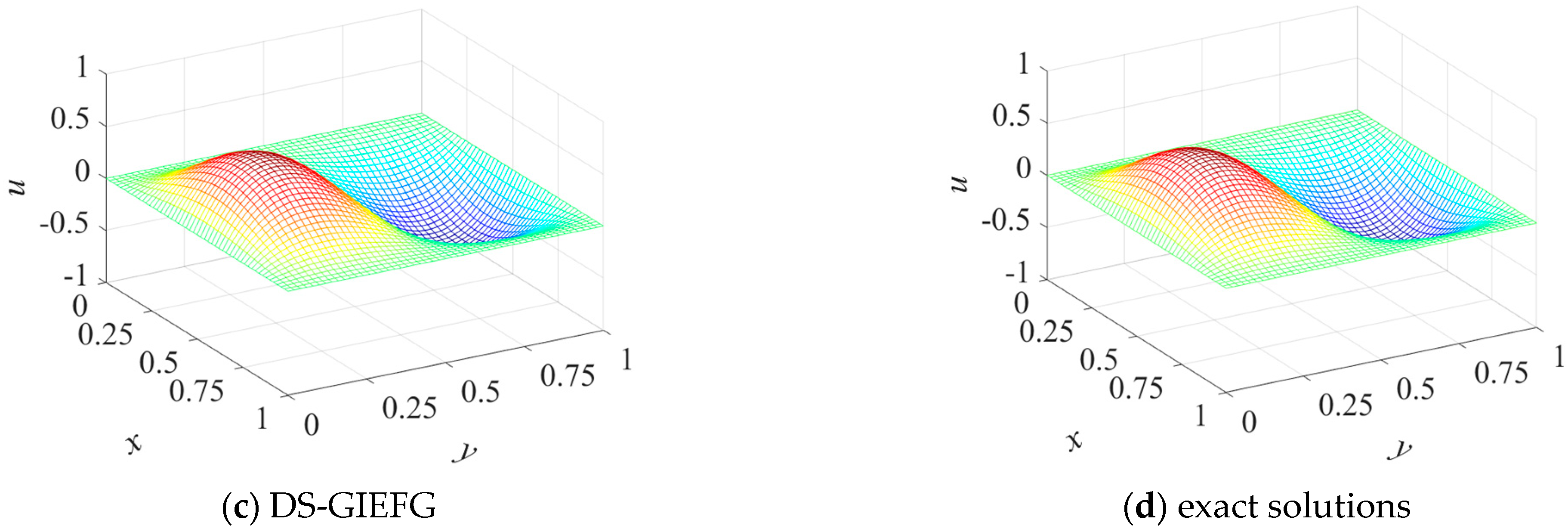
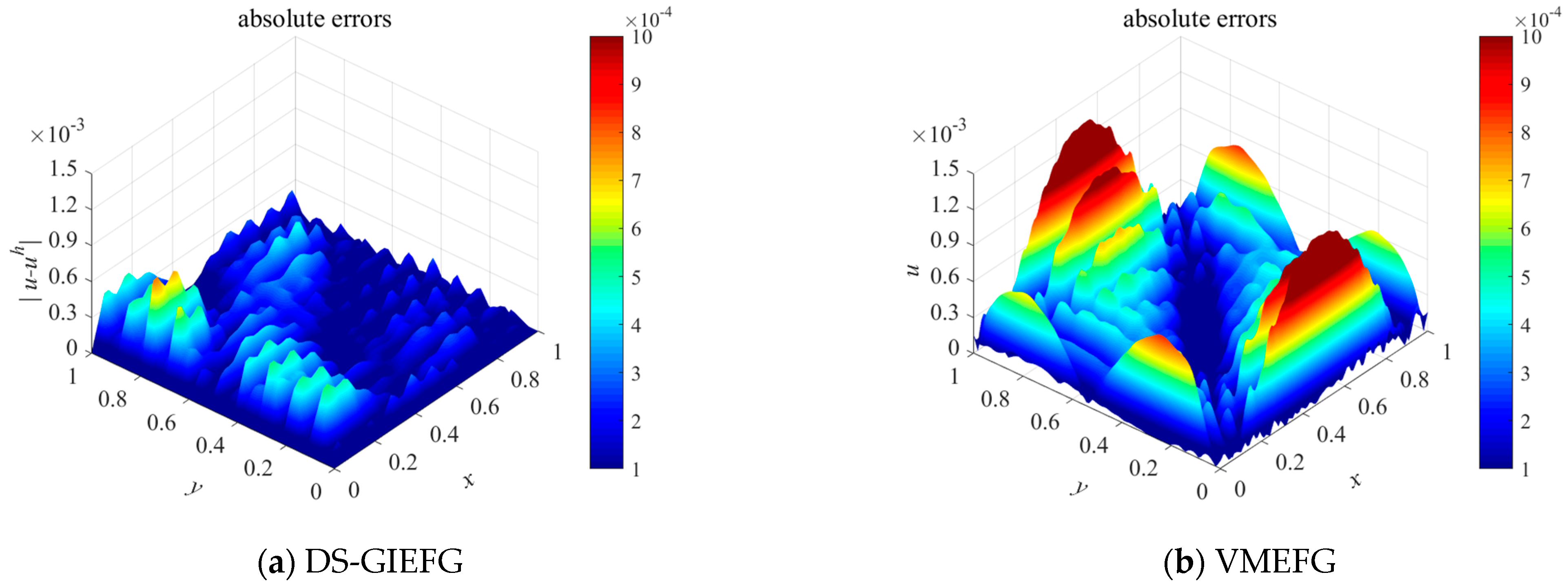
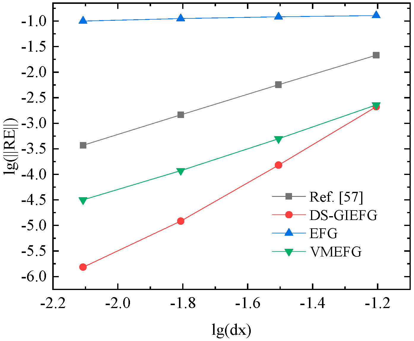
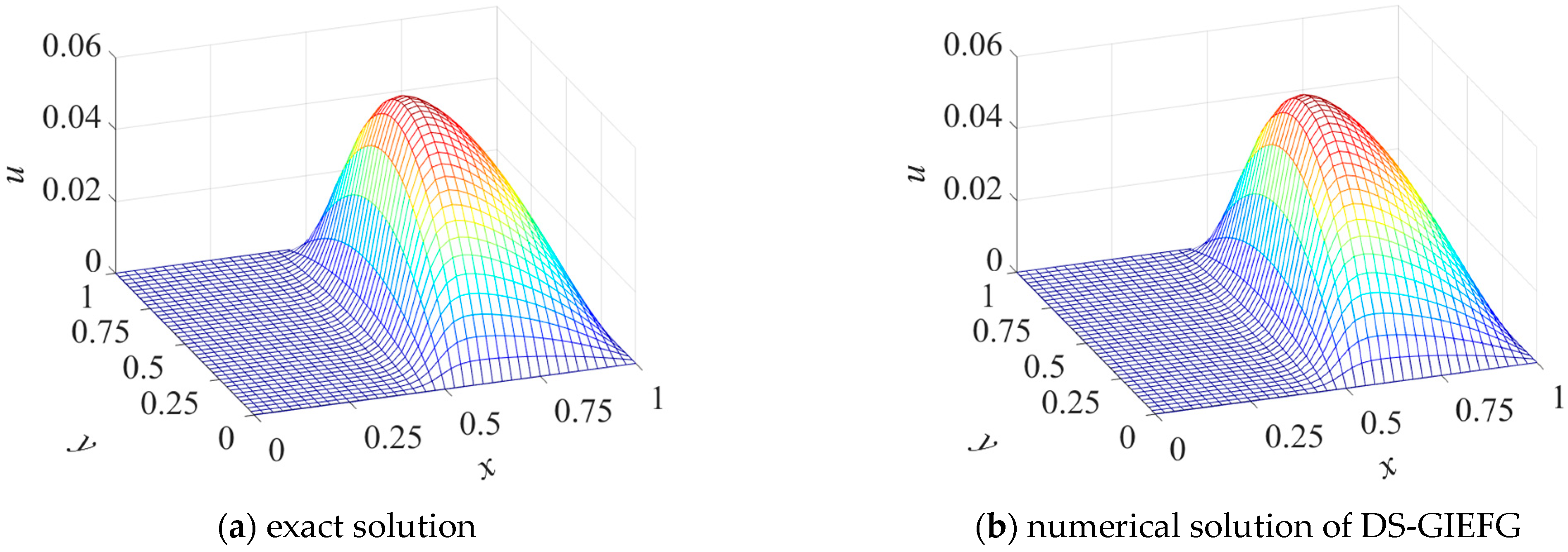
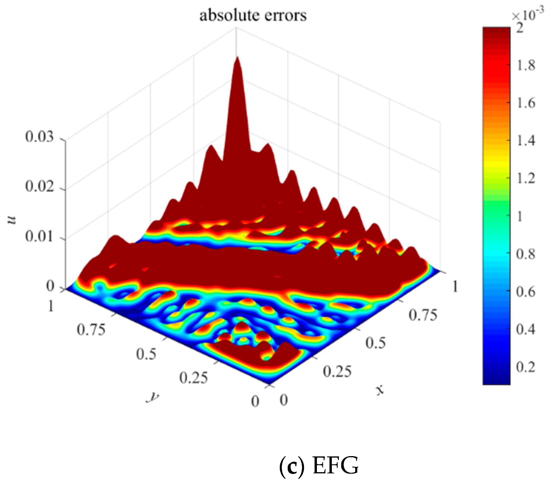
3. Numerical Examples

To show the effectiveness of the DS-GIEFG method of this paper, we will present some examples of singularly perturbed steady CDR problems. The examples wer solved on a notebook computer with I5-6200U CPU @2.30GHz, and the SUITESPARSE MATRIX SOFTWARE was also utilized to solve the discrete equations. For comparison, the EFG and VMEFG methods were applied to solve these examples. The weight functions used in this paper were the cubic spline functions, and the influence domains of the nodes in the meshless were rectangular regions with radii of d max × Δ x , where d max is a scalar constant and Δ x denotes the spacing of the nodes. A flow chart for obtaining the numerical solutions of the DS-GIEFG method is listed in Figure 1. The numerical errors are defined as:
| | RE | | = | | u u h | | L 2 ( Ω ) | | u | | L 2 ( Ω )
| | e | | = | | u u h | | L 2 ( Ω )
where u are u h denote the exact and approximated solutions, respectively.
Example 1.
The first example is a convection–diffusion problem with the following exact solution [56]:
u ( x , y ) = 65,536 729 x 3 ( 1 x ) y 3 ( 1 y ) ,   ( x , y ) Ω = [ 0 , 1 ] × [ 0 , 1 ]
The boundary conditions were extracted from the exact solution.
When 21 × 21 regular nodes distribution is used, and the parameters are ε = 10 9 , a 1 = 1 2 ,   a 2 = 1 3 , c = 0 and d max = 2.2 , the numerical solutions solved by the DS-GIEFG method on the lines x = 0.1, 0.2, , 0.9, are listed in Figure 2. We can see that the results of the DS-GIEFG method fit very well with the analytical solutions.
For comparison, the EFG and VMEFG methods were also used to solve this example, and the boundary conditions were enforced by the penalty function method with a penalty factor of α = 10 5 . The influence scalar constants in the EFG and VMEFG methods are d max = 2.8 . Then, under the 21 × 21 regular nodes distribution, the absolute errors on the whole field are shown in Figure 3. Clearly, the solution of the DS-GIEFG method has better calculation accuracy than those of the other two methods.
To show the convergence on node spacing, when 11 × 11, 21 × 21, , 51 × 51 regular node distributions were used; the relative errors of the DS-GIEFG, VMEFG and EFG methods with respect to node spacing are shown in Figure 4, and the corresponding CPU times are listed in Figure 5. Figure 4 shows that the proposed method has higher calculation accuracy and convergence order, and the numerical solution will gradually converge to the analytical solution with the reduction in node spacing. It can also be seen from Figure 5 that the proposed method has less computation time and higher computational efficiency than the EFG and VMEFG methods.
Example 2.
This example [57] is defined in the field of Ω = [ 0 , 1 ] × [ 0 , 1 ] with the exact solution of:
u ( x , y ) = 100 x 2 y ( 1 x ) 2 ( 1 y ) ( 1 2 y )
The essential boundary was used and determined by the exact solution.
The parameters were chosen to be ε = 10 8 , a 1 = a 2 = 1 , c = 0 and d max = 2.2 . When using 21 × 21 node distributions, the 3D surfaces of the solution obtained by the EFG, VMEFG and DS-GIEFG methods are, respectively, shown in Figure 6a–c, and the corresponding exact solution is plotted in Figure 6d. The penalty factor and scalar constant of influence domain in the EFG and VMEFG methods are α = 10 5 and d max = 2.6 , respectively. The corresponding snapshots of the solutions of the DS-GIEFG method on the fields of lines x = 0.1, 0.2, , 0.9 are listed in Figure 7. Additionally, the absolute errors of the DS-GIEFG and VMEFG methods on the whole field are shown in Figure 8. It can be seen from Figure 6a that the solution of the EFG method is unstable, and there is a non-physical oscillation for the diffusion convection problem with a very small diffusion coefficient. Figure 6 shows that both VMEFG and DS-GIEFG methods can obtain stable numerical solutions for small diffusion coefficients. Figure 8 also shows that the DS-GIEFG method can have higher calculation accuracy than the VMEFG method.
When the 17 × 17, 33 × 33, 65 × 65, 129 × 129 node distributions are used, the relative errors of the EFG, VMEFG and DS-GIEFG methods in the lg–lg scale are presented in Figure 9. The results of Ref. [57] are also listed in this figure. Additionally, the corresponding CPU time of these methods is plotted in Figure 10. For this example, there is no doubt that the DS-GIEFG method in this paper has higher calculation accuracy and efficiency.
Example 3.
This example is chosen to be an interior layer problem with the exact solution [58]:
u ( x , y ) = 1 2 x ( 1 x ) y ( 1 y ) ( 1 tan y a b ) ,   ( x , y ) Ω = [ 0 , 1 ] × [ 0 , 1 ]
Let ε = 10 9 , a 1 = 0 ,   a 2 = 1 ,   c = 1 ,   a = b = 0.05 . The other parameters are exactly the same as in Example 2. When using 51 × 51 nodes, the 3D surface of the exact and numerical solutions of the DS-GIEFG method are plotted in Figure 11. Additionally, the snapshots of solutions on the lines y = 0.1 , 0.2 , , 0.5 are shown in Figure 12. These two figures show that the solutions of the DS-GIEFG method are very consistent with those of the exact solutions.
When the 9 × 9, 17 × 17, 33 × 33, 65 × 65, 129 × 129 nodes distributions are used, the errors | | u u h | | of the Ref. [58], EFG, VMEFG and DS-GIEFG methods are listed in Table 1. Additionally, the corresponding variation of the errors with respect to the CPU time is shown in Figure 13. These results once again show that the method proposed in this paper has high computational accuracy and computational efficiency.

4. Conclusions

To improve the computational efficiency and overcome the non-physical oscillation of the EFG method in solving singularly perturbed fluid problems, a DS-GIEFG method for singularly perturbed steady CDR problems is proposed in this paper by constructing the trial functions based on the IIMLS method and coupling the DSM and GEFG method. The stabilization parameter of the DS-GIEFG method is only related to the nodes and not to the mesh. Since the two-dimensional problem is divided into a series of one-dimensional problems, the DS-GIEFG method has high efficiency. Three numerical examples are solved by the DS-IEFG method of this paper. The numerical solutions are compared with those of the EFG and VMEFG methods. The numerical results show that the solutions of the DS-GIEFG method converge to the analytical solution with the increase in the number of nodes, and the DS-GIEFG method has higher computational efficiency and accuracy than the EFG and VMEFG methods.

Author Contributions

Conceptualization, F.S. and J.W.; methodology, F.S. and J.W.; software, J.W. and X.K.; writing—original draft preparation, J.W. and F.S.; writing—review and editing, F.S. and R.C. All authors have read and agreed to the published version of the manuscript.

Funding

This research was funded by the Natural Science Foundation of Zhejiang Province, China (Grant Nos. LY20A010021, LY18F020026, LY19A010002), and the Ningbo Natural Science Foundation of China (Nos. 20211JCGY010257 and 202003N4142).

Data Availability Statement

Not applicable.

Conflicts of Interest

The authors declare no conflict of interest.

References

  1. Liu, Z.; Wei, G.; Wang, Z. Numerical analysis of functionally graded materials using reproducing kernel particle method. Int. J. Appl. Mech. 2019, 11, 1950060. [Google Scholar] [CrossRef]
  2. Liu, Z.; Wei, G.; Wang, Z.; Qiao, J. The meshfree analysis of geometrically nonlinear problem based on radial basis reproducing kernel particle method. Int. J. Appl. Mech. 2020, 12, 2050044. [Google Scholar] [CrossRef]
  3. Hosseini, S.; Rahimi, G. Nonlinear bending analysis of hyperelastic plates using FSDT and meshless collocation method based on radial basis function. Int. J. Appl. Mech. 2021, 13, 2150007. [Google Scholar] [CrossRef]
  4. Selim, B.A.; Liu, Z. Impact analysis of functionally-graded graphene nanoplatelets-reinforced composite plates laying on Winkler-Pasternak elastic foundations applying a meshless approach. Eng. Struct. 2021, 241, 112453. [Google Scholar] [CrossRef]
  5. Fu, Z.; Zhang, J.; Li, P.; Zheng, J. A semi-lagrangian meshless framework for numerical solutions of two-dimensional sloshing phenomenon. Eng. Anal. Bound. Elem. 2020, 112, 58–67. [Google Scholar] [CrossRef]
  6. Wang, J.; Sun, F. A hybrid variational multiscale element-free Galerkin method for convection-diffusion problems. Int. J. Appl. Mech. 2019, 11, 1950063. [Google Scholar] [CrossRef]
  7. Oruç, Ö. A meshless multiple-scale polynomial method for numerical solution of 3d convection-diffusion problems with variable coefficients. Eng. Comput. 2020, 36, 1215–1228. [Google Scholar] [CrossRef]
  8. Lancaster, P.; Salkauskas, K. Surfaces generated by moving least squares methods. Math. Comput. 1981, 37, 141–158. [Google Scholar] [CrossRef]
  9. Cheng, J. Residential land leasing and price under public land ownership. J. Urban Plan. Dev. 2021, 147, 05021009. [Google Scholar] [CrossRef]
  10. Cheng, J. Analysis of commercial land leasing of the district governments of Beijing in China. Land Use Policy 2021, 100, 104881. [Google Scholar] [CrossRef]
  11. Cheng, J. Analyzing the factors influencing the choice of the government on leasing different types of land uses: Evidence from Shanghai of China. Land Use Policy 2020, 90, 104303. [Google Scholar] [CrossRef]
  12. Cheng, J. Data analysis of the factors influencing the industrial land leasing in shanghai based on mathematical models. Math. Probl. Eng. 2020, 2020, 9346863. [Google Scholar] [CrossRef] [Green Version]
  13. Zheng, G.; Cheng, Y. The improved element-free Galerkin method for diffusional drug release problems. Int. J. Appl. Mech. 2020, 12, 2050096. [Google Scholar] [CrossRef]
  14. Belytschko, T.; Lu, Y.Y.; Gu, L. Element-free Galerkin methods. Int. J. Numer. Methods Eng. 1994, 37, 229–256. [Google Scholar] [CrossRef]
  15. Wang, J.; Sun, F.; Xu, Y. Research on error estimations of the interpolating boundary element free-method for two-dimensional potential problems. Math. Probl. Eng. 2020, 2020, 6378745. [Google Scholar] [CrossRef]
  16. Wang, J.; Wang, J.; Sun, F.; Cheng, Y. An interpolating boundary element-free method with nonsingular weight function for two-dimensional potential problems. Int. J. Comput. Methods 2013, 10, 1350043. [Google Scholar] [CrossRef]
  17. Wang, J.; Sun, F. An interpolating meshless method for the numerical simulation of the time-fractional diffusion equations with error estimates. Eng. Comput. 2019, 37, 730–752. [Google Scholar] [CrossRef]
  18. Liu, F.; Wu, Q.; Cheng, Y. A meshless method based on the nonsingular weight functions for elastoplastic large deformation problems. Int. J. Appl. Mech. 2019, 11, 1950006. [Google Scholar] [CrossRef]
  19. Nguyen, V.P.; Rabczuk, T.; Bordas, S.; Duflot, M. Meshless methods: A review and computer implementation aspects. Math. Comput. Simul. 2008, 79, 763–813. [Google Scholar] [CrossRef] [Green Version]
  20. Silling, S.A.; Lehoucq, R.B. Peridynamic theory of solid mechanics. Adv. Appl. Mech. 2010, 44, 73–168. [Google Scholar]
  21. Silling, S.A.; Askari, E. A meshfree method based on the peridynamic model of solid mechanics. Comput. Struct. 2005, 83, 1526–1535. [Google Scholar] [CrossRef]
  22. Zhang, T.; Li, X. A generalized element-free Galerkin method for stokes problem. Comput. Math. Appl. 2018, 75, 3127–3138. [Google Scholar] [CrossRef]
  23. Wang, J.; Sun, F. A hybrid generalized interpolated element-free Galerkin method for Stokes problems. Eng. Anal. Bound. Elem. 2020, 111, 88–100. [Google Scholar] [CrossRef]
  24. Zhang, T.; Li, X. A novel variational multiscale interpolating element-free Galerkin method for generalized Oseen problems. Comput. Struct. 2018, 209, 14–29. [Google Scholar] [CrossRef]
  25. Zhang, L.; Ouyang, J.; Zhang, X.; Zhang, W. On a multiscale element-free Galerkin method for the Stokes problem. Appl. Math. Comput. 2008, 203, 745–753. [Google Scholar]
  26. Abbaszadeh, M.; Dehghan, M.; Navon, I.M. A proper orthogonal decomposition variational multiscale meshless interpolating element-free Galerkin method for incompressible magnetohydrodynamics flow. Int. J. Numer. Methods Fluids 2020, 92, 1415–1436. [Google Scholar] [CrossRef]
  27. Zhang, X.; Zhang, P.; Qin, W.; Shi, X. An adaptive variational multiscale element free Galerkin method for convection–diffusion equations. Eng. Comput. 2021, 1–18. [Google Scholar] [CrossRef]
  28. Dehghan, M.; Abbaszadeh, M. Variational multiscale element free Galerkin (VMEFG) and local discontinuous Galerkin (LDG) methods for solving two-dimensional brusselator reaction–diffusion system with and without cross-diffusion. Comput. Methods Appl. Mech. Eng. 2016, 300, 770–797. [Google Scholar] [CrossRef]
  29. Meng, Z.; Cheng, H.; Ma, L.; Cheng, Y. The dimension splitting element-free Galerkin method for 3d transient heat conduction problems. Sci. China Phys. Mech. 2019, 62, 1–12. [Google Scholar] [CrossRef]
  30. Wu, Q.; Peng, M.J.; Fu, Y.D.; Cheng, Y.M. The dimension splitting interpolating element-free Galerkin method for solving three-dimensional transient heat conduction problems. Eng. Anal. Bound. Elem. 2021, 128, 326–341. [Google Scholar] [CrossRef]
  31. Cheng, H.; Peng, M.; Cheng, Y.; Meng, Z. The hybrid complex variable element-free Galerkin method for 3d elasticity problems. Eng. Struct. 2020, 219, 110835. [Google Scholar] [CrossRef]
  32. Li, K.; Huang, A.; Zhang, W.L. A dimension split method for the 3-d compressible Navier–Stokes equations in turbomachine. Commun. Numer. Methods Eng. 2002, 18, 1–14. [Google Scholar] [CrossRef]
  33. Wu, Q.; Peng, M.; Cheng, Y. The interpolating dimension splitting element-free Galerkin method for 3d potential problems. Eng. Comput. 2021, 1–15. [Google Scholar] [CrossRef]
  34. Meng, Z.J.; Cheng, H.; Ma, L.D.; Cheng, Y.M. The dimension split element-free Galerkin method for three-dimensional potential problems. Acta Mech. Sin. 2018, 34, 462–474. [Google Scholar] [CrossRef]
  35. Bansal, K.; Sharma, K.K. Parameter uniform numerical scheme for time dependent singularly perturbed convection-diffusion-reaction problems with general shift arguments. Numer. Algorithms 2017, 75, 113–145. [Google Scholar] [CrossRef]
  36. Kaya, A. Finite difference approximations of multidimensional unsteady convection-diffusion-reaction equations. J. Comput. Phys. 2015, 285, 331–349. [Google Scholar] [CrossRef] [Green Version]
  37. Zhao, S.; Xiao, X.; Tan, Z.; Feng, X. Two types of spurious oscillations at layers diminishing methods for convection-diffusion–reaction equations on surface. Numer. Heat. Transf. A Appl. 2018, 74, 1387–1404. [Google Scholar] [CrossRef]
  38. Han, H.; Huang, Z. Tailored finite point method based on exponential bases for convection-diffusion-reaction equation. Math. Comput. 2013, 82, 213–226. [Google Scholar] [CrossRef]
  39. Lin, R.; Ye, X.; Zhang, S.; Zhu, P. A weak Galerkin finite element method for singularly perturbed convection-diffusion-reaction problems. SIAM J. Numer. Anal. 2018, 56, 1482–1497. [Google Scholar] [CrossRef]
  40. Fendoğlu, H.; Bozkaya, C.; Tezer-Sezgin, M. Dbem and DRBEM solutions to 2d transient convection-diffusion-reaction type equations. Eng. Anal. Bound. Elem. 2018, 93, 124–134. [Google Scholar] [CrossRef]
  41. Lukyanenko, D.V.; Shishlenin, M.A.; Volkov, V.T. Asymptotic analysis of solving an inverse boundary value problem for a nonlinear singularly perturbed time-periodic reaction-diffusion-advection equation. J. Inverse Ill Posed Probl. 2019, 27, 745–758. [Google Scholar] [CrossRef]
  42. Lukyanenko, D.V.; Grigorev, V.B.; Volkov, V.T.; Shishlenin, M.A. Solving of the coefficient inverse problem for a nonlinear singularly perturbed two-dimensional reaction—Diffusion equation with the location of moving front data. Comput. Math. Appl. 2019, 77, 1245–1254. [Google Scholar] [CrossRef]
  43. Chandru, M.; Das, P.; Ramos, H. Numerical treatment of two-parameter singularly perturbed parabolic convection diffusion problems with non-smooth data. Math. Methods Appl. Sci. 2018, 41, 5359–5387. [Google Scholar] [CrossRef]
  44. Wu, Y.; Zhang, N.; Yuan, J. A robust adaptive method for singularly perturbed convection-diffusion problem with two small parameters. Comput. Math. Appl. 2013, 66, 996–1009. [Google Scholar] [CrossRef]
  45. Kaya, A.; Sendur, A. Finite difference approximations of multidimensional convection–diffusion–reaction problems with small diffusion on a special grid. J. Comput. Phys. 2015, 300, 574–591. [Google Scholar] [CrossRef] [Green Version]
  46. Lin, J.; Reutskiy, S. A cubic b-spline semi-analytical algorithm for simulation of 3d steady-state convection-diffusion-reaction problems. Appl. Math. Comput. 2020, 371, 124944. [Google Scholar] [CrossRef]
  47. Gharibi, Z.; Dehghan, M. Convergence analysis of weak Galerkin flux-based mixed finite element method for solving singularly perturbed convection-diffusion-reaction problem. Appl. Numer. Math. 2021, 163, 303–316. [Google Scholar] [CrossRef]
  48. Lin, J.; Reutskiy, S.Y.; Lu, J. A novel meshless method for fully nonlinear advection–diffusion-reaction problems to model transfer in anisotropic media. Appl. Math. Comput. 2018, 339, 459–476. [Google Scholar] [CrossRef]
  49. Hidayat, M.I.P. Meshless finite difference method with b-splines for numerical solution of coupled advection-diffusion-reaction problems. Int. J. Therm. Sci. 2021, 165, 106933. [Google Scholar] [CrossRef]
  50. Zhang, X.; Xiang, H. Variational multiscale element free Galerkin method for convection-diffusion-reaction equation with small diffusion. Eng. Anal. Bound. Elem. 2014, 46, 85–92. [Google Scholar] [CrossRef]
  51. Zhang, P.; Zhang, X.; Xiang, H.; Song, L. A fast and stabilized meshless method for the convection-dominated convection-diffusion problems. Numer. Heat. Transf. A Appl. 2016, 70, 420–431. [Google Scholar] [CrossRef]
  52. Li, J.; Feng, X.; He, Y. Rbf-based meshless local Petrov Galerkin method for the multi-dimensional convection-diffusion-reaction equation. Eng. Anal. Bound. Elem. 2019, 98, 46–53. [Google Scholar] [CrossRef]
  53. Wang, F.; Wang, C.; Chen, Z. Local knot method for 2d and 3d convection–diffusion–reaction equations in arbitrary domains. Appl. Math. Lett. 2020, 105, 106308. [Google Scholar] [CrossRef]
  54. Liu, S.; Li, P.; Fan, C.; Gu, Y. Localized method of fundamental solutions for two-and three-dimensional transient convection-diffusion-reaction equations. Eng. Anal. Bound. Elem. 2021, 124, 237–244. [Google Scholar] [CrossRef]
  55. Dehghan, M.; Abbaszadeh, M. Proper orthogonal decomposition variational multiscale element free Galerkin (POD-VMEFG) meshless method for solving incompressible Navier–Stokes equation. Comput. Methods Appl. Mech. Eng. 2016, 311, 856–888. [Google Scholar] [CrossRef]
  56. Zhang, T.; Li, X. A variational multiscale interpolating element-free Galerkin method for convection-diffusion and stokes problems. Eng. Anal. Bound. Elem. 2017, 82, 185–193. [Google Scholar] [CrossRef]
  57. Chen, G.; Feng, M.; Xie, C. A new projection-based stabilized method for steady convection-dominated convection-diffusion equations. Appl. Math. Comput. 2014, 239, 89–106. [Google Scholar] [CrossRef]
  58. Gao, F.; Zhang, S.; Zhu, P. Modified weak Galerkin method with weakly imposed boundary condition for convection-dominated diffusion equations. Appl. Numer. Math. 2020, 157, 490–504. [Google Scholar] [CrossRef]
Figure 1. A flow chart for obtaining the numerical solutions of the DS-GIEFG method.
Mathematics 09 02524 g001
Figure 2. The numerical solutions of the DS-GIEFG method with the 21 × 21 regular nodes and ε = 10 9 , a 1 = 1 / 3 ,   a 2 = 1 / 2 .
Mathematics 09 02524 g002
Figure 3. Absolute errors of the solutions solved by the (a) DS-GIEFG method, (b) VMEFG method and (c) EFG method with the same conditions of Figure 2.
Mathematics 09 02524 g003aMathematics 09 02524 g003b
Figure 4. The variation of relative errors of the DS-GIEFG, VMEFG and EFG methods with respect to node spacing (in lg–lg scale).
Mathematics 09 02524 g004
Figure 5. The variation of relative errors of the DS-GIEFG, VMEFG and EFG methods with respect to the CPU time (in lg–lg scale).
Mathematics 09 02524 g005
Figure 6. The exact solutions and the numerical solutions obtained by the EFG, VMEFG and DS-GIEFG methods.
Mathematics 09 02524 g006aMathematics 09 02524 g006b
Figure 7. The snapshots of numerical solutions of the DS-GIEFG method on the lines of x = 0.1 , 0.2 , , 0.9 with 21 × 21 nodes.
Mathematics 09 02524 g007
Figure 8. The absolute errors of the VMEFG and DS-GIEFG methods on the whole field under 21 × 21 nodes.
Mathematics 09 02524 g008
Figure 9. The variation of relative errors of different methods with respect to the node spacing (in lg–lg scale).
Mathematics 09 02524 g009
Figure 10. The variation of relative errors of different methods with respect to the CPU time (in lg–lg scale).
Mathematics 09 02524 g010
Figure 11. The exact and numerical solutions of the DS-GIEFG method with 51 × 51 regular nodes.
Mathematics 09 02524 g011
Figure 12. The snapshots of numerical solutions of the DS-GIEFG method on the lines of y = 0.1 , 0.2 , , 0.5 with 51 × 51 nodes.
Mathematics 09 02524 g012
Figure 13. The variation of errors of different methods with respect to the CPU time (in lg–lg scale).
Mathematics 09 02524 g013
Table 1. The errors | | u u h | | of the Ref. [58], EFG, VMEFG and DS-GIEFG methods for different nodes spacing.
NodesDS-GIEFGVMEFGEFGRef. [58]
9 × 97.90 × 1041.10 × 10−14.02 × 10−13.80 × 10−3
17 × 171.81 × 10−41.36 × 10−21.14 × 10−11.31 × 10−3
33 × 331.37 × 10−54.74 × 10−45.29 × 10−34.37 × 10−4
65 × 659.46 × 10−86.91 × 10−53.89 × 10−41.16 × 10−4
129 × 1291.29 × 10−81.52 × 10−57.75 × 10−52.96 × 10⁻⁵
Publisher’s Note: MDPI stays neutral with regard to jurisdictional claims in published maps and institutional affiliations.

