Abstract
For multidimensional dependent cases with incomplete probability information of random variables, global sensitivity analysis (GSA) theory is not yet mature. The joint probability density function (PDF) of multidimensional variables is usually unknown, meaning that the samples of multivariate variables cannot be easily obtained. Vine copula can decompose the joint PDF of multidimensional variables into the continuous product of marginal PDF and several bivariate copula functions. Based on Vine copula, multidimensional dependent problems can be transformed into two-dimensional dependent problems. A novel Vine copula-based approach for analyzing variance-based sensitivity measures is proposed, which can estimate the main and total sensitivity indices of dependent input variables. Five considered test cases and engineering examples show that the proposed methods are accurate and applicable.
1. Introduction
Variance-based global sensitivity analysis (GSA) is very commonly used in the area of structural safety [1,2,3]. It can calculate the contribution of each input variable or group variables to the variance of the output response, thus allowing for selection of the important variables that have great influence on the output, while the randomness of unimportant variables can be ignored. Several methods exist to perform variance-based GSA of model outputs when the inputs are independent [2,3,4,5,6], but it is still a challenge for the dependent cases.
For dependent input variables, there are some techniques proposed to solve Sobol’ indices. Xu and Gertner [7] divided the contribution of inputs into two components: the independent and dependent contributions, and proposed a regression-based method for estimating different contributions of the inputs. Similarly, Li et al. [8] introduced a unified framework including covariance in the decomposition of the model output variance, which can distinguish the structural and correlative contribution of a nominal input. Kala [9] performed GSA based on entropy, and proposed a novel method from differential entropy to alternative measures. Kucherenko et al. [10] applied a Gaussian copula method to variance-based global sensitivity analysis, and introduced a more general approach. On this basis, Song et al. [11] proposed using an adaptive copula method to solve Sobol’ indices, which can describe different types of correlations. The above methods are mainly aimed at the case of bivariate correlation. Yet, considering that many input variables are multidimensional and interrelated in engineering problems, it is necessary to propose an effective method with which to measure multidimensional correlation.
Over the past few years, the Nataf model proposed by Kiureghian et al. [12] has been widely used in structural safety engineering with multidimensional correlated variables. Lebrun and Dutfoy [13] proved that the Nataf model is essentially equivalent to multivariate Gaussian copula. Besides, Eryilmaz [14] studied multivariate Archimedean copula and applied multivariate Clayton and Gumbel copulas to the reliability analysis of weighted-k-out-of-n systems with dependent components. Daul et al. [15] discussed the grouped t-copula with an application to credit risk. Cossette et al. [16] reviewed the Farlie-Gumbel-Morgenstern (FGM) copula and expanded it to multidimensional situations. The above copula methods require that the correlations between different variables conform to the same copula function. However, many of the multidimensional variables in practical engineering have different correlations. For example, in the variable-amplitude load fatigue problem, the fatigue life under different stress levels has different correlations [17]. In flood frequency analysis, the flood peak value, total amount and duration are complexly correlated [18]. For such problems, the above multivariate copula models are subject to errors [19], and the correlations should be measured by different copula functions.
In this paper, we introduce Vine copula [20,21,22] to the variance-based global sensitivity analysis of complex multidimensional correlation problems. Vine copula can decompose the joint PDF of multidimensional variables into some bivariate copula functions of original variables and conditional variables [20], so as to measure different correlations among the multivariate variables with different copula functions. After the decomposition, the Akaike Information Criterion (AIC) method [23] or one of other methods [24,25] is required to select the optimal bivariate copula function, which can separately measure the correlation among the input variables. For engineering problems with multidimensional correlated variables, the Vine copula method can use optimal copula to separately measure the correlation of different variables. Thus, the complex dependence structure of variables can be fitted to the maximum extent, and the most accurate possible solution of and can be obtained. Due to the excellent properties of Vine copula, it has been applied in structural safety and reliability. Torre et al. [26] formalized the framework needed to build Vine copula models of multivariate inputs and combine them with virtually any uncertainty quantification method. Nazih et al. [27] studied the specific problem of structural reliability as an application of Vine copula. Sarazin et al. [28] used Vine copula to perform reliability-oriented sensitivity analysis in the presence of data-driven epistemic uncertainty. Inspired by the above works, we applied Vine copula to perform variance-based sensitivity analysis.
This paper is organized as follows: Section 2 presents a detailed introduction of Vine copula, including its basic theory and classification. The process of solving variance-based global sensitivity analysis based on Vine copula is introduced in Section 3. Section 4 analyzes some numerical and engineering tests. Conclusions are summarized in Section 5.
2. Vine Copula
Vine copula is an efficient mathematical tool to decompose the multidimensional joint PDF into the continuous product of several two-dimensional copula functions and marginal PDF [20]. Consider a set of n-dimensional correlated variables , the joint PDF of that can be decomposed as follows:
where is the marginal PDF of the input variable and is the conditional PDF of under constraint. For the multidimensional independent cases, , i.e., the joint PDF of the variables is equal to the product of marginal PDFs.
For the case of two-dimensional variables, the joint PDF is and the conditional PDF and be expressed as:
where is copula density function of input variables and , while is the marginal CDF of .
For the case of high-dimensional variables, the decomposition of Equation (1) is not unique. Bedford and Cooke [20,21] proposed Vine copula to describe the different decomposition methods and introduced a regular Vine (R-Vine) structure, in which C-Vine and D-Vine are two common structures. C-Vine can be well used to describe correlations among variables when a particular variable is known to be a key variable that governs interactions in the dataset (e.g., is the key variable of C-Vine in Figure 1), while D-Vine is suitable for describing correlated variables of the same status. An n-dimensional Vine copula model consists of trees , which has nodes and sides. Each node represents an unconditional or conditional variable, and each side represents a two-dimensional copula density function. The nodes in tree are made up of the sides in tree and related only to the sides that have a common node in tree . According to the logical structure of C-Vine and D-Vine models, the joint PDF of n-dimensional variables can, respectively, be expressed as Equations (3) and (4):
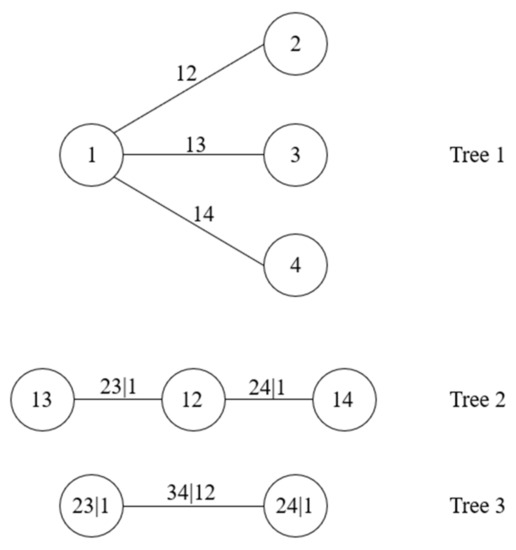
Figure 1.
C-Vine model of four-dimensional variables.
Figure 1 and Figure 2 show the structural diagrams of C-Vine and D-Vine with four dimensional variables; the corresponding decomposition of the joint PDF in Figure 1 and Figure 2 can be expressed separately as follows. It can be seen that the notation of D-Vine resembles independence graphs more than that of C-Vine. Therefore, we mainly adopted C-Vine in order to emphasize the influence of dependence on sensitivity indices.
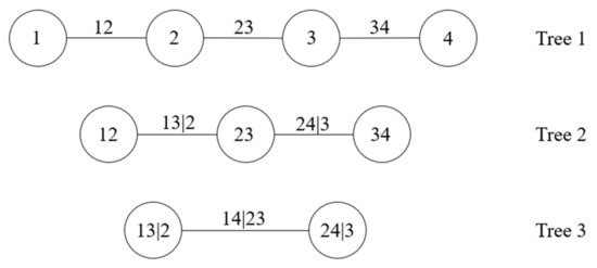
Figure 2.
D-Vine model of four-dimensional variables.
The above decomposition process involves conditional distribution and . For the convenience of expression, we introduce the function to express the binary conditional distribution, while denotes the inverse function of .
where and are the marginal cumulative distribution functions (CDF) of and , denotes copula function and denotes the parameter of copula function, which can be estimated by the AIC method [23] or other methods [24,25]. Table 1 lists the and functions of some common copula functions [29].

Table 1.
The functions h and of some frequently-used copula functions.
According to the decomposition process in Equation (3) or (4), the multidimensional joint PDF can be transformed into the product of marginal PDF and several binary copula functions. Thus, we can use the conventional binary copula functions for variance-based global sensitivity analysis with multidimensional correlated input variables.
3. Variance-Based GSA Based on Vine Copula
Considering a model function defined in with an input vector , Sobol [1] and Saltelli [2] put forward the variance-based global sensitivity indices based on ANalysis Of VAriance (ANOVA) decomposition:
where denotes the variance of model output , while and are the conditional variances of under constraint. The full expressions for and are given by the following formulas:
where denotes the expectation of model output , and where the variance is given by . Kucherenko et al. [10] derived the formula of variance-based global sensitivity indices under correlated variables based on the conditional variance theory:
where and are unconditional sample matrices generated according to the joint PDF of input variables, while and are conditional samples generated by conditional PDFs and , respectively. Tarantola and Mara [30] indicated that measures the amount of variance of due to and its dependence with but does not include the interactions of them, while accounts for the contributions of and its dependence with by ignoring the correlations among variables. Therefore, the dependence among variables may lead to (dependent effects larger than interacted effects). By comparing the values of the two indices, we can get the independent contributions, dependent contributions and interacted contributions of the variables, so as to perform factor ranking/fixing, variance cutting, etc.
According to Equations (12) and (13), Song et al. [11] introduced two copula-based methods for solving and under the case of two-dimensional correlated variables. The first method uses the copula function to approximate the real joint distribution, while the other approach uses the copula function to decompose the joint PDF into the product of the marginal PDF and copula PDF. Song et al. [11] also concluded that the second method is less computationally efficient than the first method, so we mainly discuss the first copula-based method in this paper. For the sake of description, we denote the two methods based on Vine copula as VC1 and VC2. In this section, we extend VC1 to the case of multidimensional correlation, where there is a need to decompose the joint PDF of the input variables into the product of several two-dimensional copula functions and marginal PDF using the Vine copula function (details of VC2 are presented in Appendix A).
The basic idea of VC1 is to use the copula function to approximate the real joint distribution, and generate unconditional and conditional samples according to the selected optimal copula function. This method can rewrite (12) and (13) as follows:
where N is the number of samples. After the decomposition of the joint PDF with the Vine copula function, each optimal two-dimensional copula function and its parameters needs to be inferred by using the known samples. According to the selected optimal copula function, we generate samples according to the following ideas and steps [20,31].
Assuming that is a group of samples of input variables , according to Rosenblatt model [32], the marginal and conditional distribution of can be expressed as follows:
where are independent and uniformly distributed between 0 and 1. Correspondingly, we can get the inverse transform of Equation (16).
Assuming that are the marginal CDF values of the input variables, i.e., , the sampling procedure is as follows:
- Generate two independent vectors, and , uniformly distributed between 0 and 1;
- Let , and obtain ;
- Let , and obtain , ;
- Let , and obtain , ;
- Take the iteration repeatedly, and get a group of unconditional samples .
Considering the above sampling method involves a conditional copula function, the generation of conditional samples is similar to the above procedure. There is just a need to construct independent uniform variables as and , and thus the specific steps are omitted. The above procedure can be briefly summarized as in the following figure. After getting the unconditional and conditional samples, and can be computed according to Equations (14) and (15). The solution process is concluded as Figure 3.
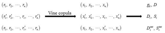
Figure 3.
The solution process of VC1.
4. Test Cases
In this section, the developed approach is illustrated by five different models with multidimensional correlated input variables.
The first test with lognormal distributed variables’ numerical solutions is computed and compared with the reference results. We also compare the solutions obtained by the two copula-based methods and discuss the effect of different Vine copulas on the results. Test 2 compares the results obtained by the developed approach and traditional Nataf model by analyzing a four-dimensional dependent model. The third case’s variables are uniformly distributed and the influence of Kendall on the results is analyzed. The last two tests are engineering cases with complex model functions and correlations, in which Test 5 combines the proposed method and the finite element models.
4.1. Test 1. Example with Complete Probability Information
Consider a model function
where the input variables are normally distributed variables with , . The linear correlation coefficients are , so that the covariance matrix is . According to the theory of multivariate normal distribution [10], a sufficient number of samples can be generated to accurately estimate the mean and variance of the output response.
Further, we assume the input variables to have lognormal distribution with parameters and . By exponent transformation of the above normally distributed samples , we can obtain the lognormal distributed samples with unknown correlations, which are used for copula parameter estimation, and the optimal copula functions can be selected by the AIC method. The results are shown in Table 2, and the AIC values of the optimal copula are marked in bold.
Table 2.
The results of parameter estimation and AIC method.
Table 2 shows that the optimal bivariate copula functions among all variables are Gaussian copula, so we use bivariate Gaussian copula to construct Vine copula. The results obtained by the two methods based on the Vine copula function are listed in Table 3, while the reference solutions obtained by exponential transformation and the approximate solutions based on the Nataf model are also listed in Table 3.
Table 3.
Values of , D, and .
Table 3 shows that the two Vine copula methods obtain almost the same results as reference solutions, which illustrates the feasibility and accuracy of the developed methods. For this case, Vine copula consists only of Gaussian copula functions, which means Vine copula is essentially the same as the Nataf model (multivariate Gaussian copula) for this model. Therefore, the results obtained by Vine copula methods and Nataf methods are very close.
Furthermore, we notice that the results obtained by VC2 need more sample points than VC1 but have less accuracy. The convergence curve of the results obtained by the two methods with the number of samples is shown in Figure 4. We can see that the convergence of VC1 is better than that of VC2, which is consistent with the previous conclusion of Song et al. [11]. This may be because VC2 needs to calculate the copula density function when calculating Sobol’ indices, which may lead to numerical errors and cause abrupt changes in the results. Therefore, we only discuss VC1 in the following tests.
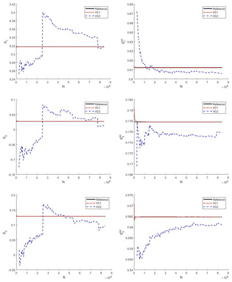
Figure 4.
Convergence plots of the methods for and .
The above method uses C-Vine to construct the joint PDF of input variables ( as the key variable), i.e., the two-dimensional variables required for sampling are , and . We change the key variable and use a different C-Vine structure to describe the joint distribution of variables. The values of and D obtained by C-Vine copulas with different key variables are listed in Table 4. It can be seen that almost the same results can be obtained by different C-Vine copulas, which means C-Vine copulas based on different key variables have little effect on the mean and variance of the output response for this model.
Table 4.
Values of and D obtained by different C-Vine copulas ().
4.2. Test 2. Portfolio Model
Consider the Portfolio model [10]:
The input variables are normally distributed with and . There are several known samples () in Figure 5, which shows all the variables are correlated.
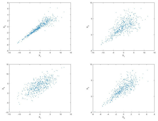
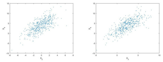
Figure 5.
Sample distribution of input variables ().
According to Equation (5), the four-dimensional input variables are decomposed as six two-dimensional variables: , , , , and . The AIC values of each alternative bivariate copula function are listed in Table 5, which were calculated by using the above 500 samples. We mark the AIC values of the optimal copula in bold and display the corresponding parameters in Table 5.
Table 5.
Values of parameter estimation and AIC method ().
It can be seen that the optimal copula functions of two-dimensional variables are Clayton copula, Gaussian copula and Frank copula. Thus, there will be unknown errors if using the traditional Nataf method to measure the correlation. Table 6 gives the values obtained by the Nataf method and VC1.
Table 6.
Values of , D, and ().
The results obtained by the traditional Nataf method and the proposed Vine copula method are different, as well as the importance orders of input variables. According to the values of , the Nataf method gives the importance order of input variables as , while is obtained if using the Vine copula method. Considering that an accurate importance order of variables is vital in practical problems, if we only use the conventional Nataf method for this problem, inaccurate results may be obtained, thus affecting the structural safety of a design.
Figure 6 shows the distribution of the samples of the two methods. It can be seen that the samples generated by the Nataf method have symmetry but no tail correlation, while the Vine copula samples show a significantly lower tail correlation, which perfectly matches the distribution of variables and in Figure 5. This model illustrates that the tail correlation of variables has great impacts on Sobol’ indices. Since the traditional Nataf method cannot capture the tail correlation between variables, the estimated results of the Nataf method will have unknown errors if there is obvious tail correlation between the variables, which is also the reason for the large gap between the results of the Nataf method and the Vine copula method for this model.
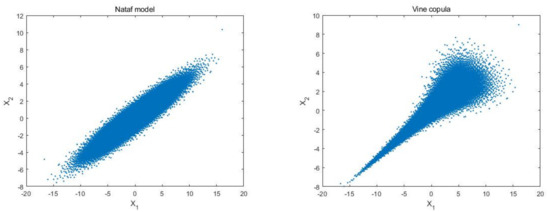
Figure 6.
Sample distribution generated by two methods (, ).
Furthermore, it can be seen that for this model, which means the correlations among input variables have greater effects than interactions on the variance of the output. Therefore, we should focus on the main indices in practical engineering when analyzing correlations, especially for non-normally dependent and nonlinear problems.
4.3. Test 3. Ishigami Function
Consider the Ishigami function [10]:
with input variables being uniformly distributed: . This function is widely used as a benchmark for sensitivity analysis since it has strong non-linearity and non-monotonicity.
We also analyzed this model in [11] and considered that only the variables and are dependent. In this paper, we assume that the three input variables are all correlated, and the distribution of 500 samples of input variables is shown in Figure 7. It can be seen that there is upper tail correlation between and , and lower tail correlation between and .
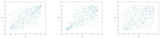
Figure 7.
Sample distribution of input variables ().
By using the above samples, the optimal copula functions and their parameters among the two-dimensional variables are selected by the AIC method, and the results are listed in Table 7 (where the AIC values of the optimal copula functions are in bold).
Table 7.
Values of parameter estimation and AIC method ().
The optimal copula functions between two-dimensional variables are mainly Clayton copula and Gumbel copula, the parameters of which are listed in Table 7. Table 8 gives the values obtained by the Nataf method and the proposed method. It is shown that the importance orders of variables obtained by the two methods are the same (), but the specific values of and are different. This is because the Vine copula method proposed in this paper takes into account the tail correlation between variables, which cannot be measured by the Nataf method.
Table 8.
Values of , D, and ().
We also analyze the influence of degree of correlation of input variables on the importance analysis results. It is assumed that the Kendall between the decomposed two-dimensional variables is the same, and the optimal copula functions in the previous step are used. The proposed Vine copula method and Nataf method are used for analysis, and the independent situation of the three variables is considered at the same time. The curve of the calculated results changing with Kendall is shown in Figure 8.
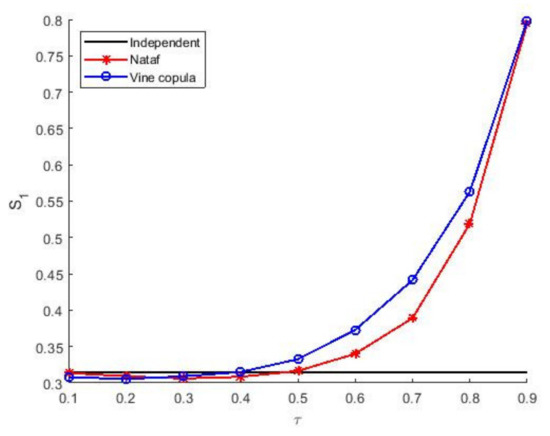
Figure 8.
Values of obtained by two methods versus .
It can be seen that the results obtained by the two methods show the same trend with Kendall and are significantly different from the results in the independent case. This shows that the correlation between variables has a great impact on the Sobol’ indices. If the variables are simply assumed as independent variables for processing, this may cause a large error in the importance analysis and affect the safety of designs in engineering. Besides, the results obtained by the two methods are relatively close in the case of small and large Kendall , while the results are significantly different when . This indicates that the Vine copula method with better correlation measurement should be selected for analysis within the correlation range .
4.4. Test 4. Fatigue and Creep of Materials
Fatigue and the creep of materials are two common failure modes at high temperatures. Based on experimental data using the linear damage accumulation rule, Mao et al. [33] proposed a probabilistic model for reliability analysis of the creep and fatigue of materials as follows:
where and denote the creep damage and fatigue damage, respectively, and and are the parameters obtained from the experimental results. Two instances of damage can be expressed as and , where and correspond to the creep life and fatigue life, respectively, while and are the number of the creep and fatigue load cycles.
Assuming that the creep and fatigue lifetimes of a material follow log-normal distribution, and are normally distributed. The assumed values of the distribution parameters are shown in Table 9.
Table 9.
Values and distribution parameters of input variables.
The input variables , , and are dependent according to the theory of material mechanics. There are several experimental data, the distributions of which are shown in Figure 9. The sample values of and can be calculated by using these data. Figure 10 shows the curve of creep-fatigue failure.
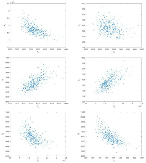
Figure 9.
Sample distribution of input variables ().
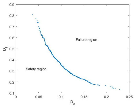
Figure 10.
Creep-fatigue failure function.
Figure 10 shows that the relationship between creep damage and fatigue damage is nonlinear, i.e., the ultimate damage to the material is a nonlinear function of fatigue damage and creep damage, which means creep damage and fatigue damage affect each other. The contribution of each input variable to the limit state equation is analyzed. The samples in Figure 9 are statistically inferred to determine the optimal copula function and correlation parameters between the two-dimensional variables by the AIC method. The results are listed in Table 10.
Table 10.
Values of parameter estimation and AIC method ().
Figure 11 gives the results of variance-based global sensitivity indices with the Nataf method and Vine copula method. It can be seen that the results obtained by the two methods are relatively similar, and the same importance order of variables is obtained. According to the values of in Figure 11a, the fatigue life and the fatigue load cycle have greater influences on the limit state function than and , which is consistent with the AIC values in Table 10. This means the effects of input variables can be predicted preliminarily after the correlation estimation by the AIC method. For the parameters in the experiment, the influence of is greater than . We can conclude that the fatigue life and fatigue load cycle of materials most affect the creep-fatigue failure of the structure.
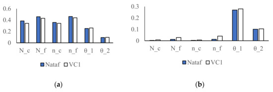
Figure 11.
The values of Sobol’ indices; (a) , (b) .
In addition, the importance measurement results obtained by the two methods are different since the Vine copula method uses the optimal copula (Gaussian copula and Frank copula, respectively) to measure the correlation between variables, while the traditional Nataf method only uses a single Gaussian copula to compute.
4.5. Test 5. Three-Bay Five-Story Linear Elastic Frame Structure
Consider a three-bay five-story linear elastic frame structure [34,35], as shown in Figure 12, which is characterized by 21 random variables: 3 applied loads, 2 Young’s moduli, 8 moments of inertia and 8 cross-sectional areas. The properties of the frame structures and the distribution types and parameters of random variables are given in Table 11 and Table 12, respectively. Statistical dependence among the basic variables is considered. All loads are correlated with linear correlation coefficient , while the cross-sectional area and the moment of inertia of each element type are correlated with . All cross-sectional properties are correlated as
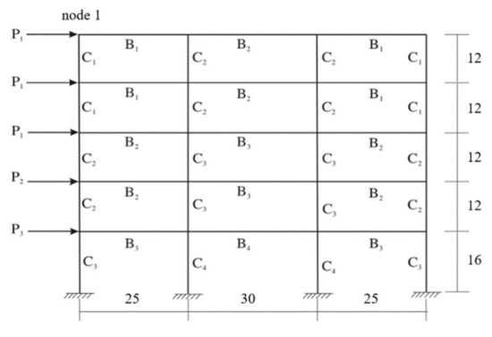
Figure 12.
Three-bay five-story linear elastic frame structure.
Table 11.
Properties of the frame structures.
Table 12.
Statistical properties of random variables.
We consider the horizontal displacement at node 1 as output function:
where denotes the actual horizontal displacement as an implicit function of all basic variables.
According to engineering qualitative analysis, input variables , , , , , and contribute more than 95% to the output variance. Thus, we mainly analyze the importance orders of these seven input variables. In the following, the frame structure is modeled and analyzed by ANSYS with element type BEAM188. Several samples () are generated using the Nataf model with the linear correlation coefficients. According to these samples, Gaussian copula is selected as the optimal bivariate copula of the Vine structure through the AIC method, and the corresponding parameters are computed as well (given in Appendix B). The values of Sobol’ indices given by the Nataf method and Vine copula method are listed in Table 13.
Table 13.
Values of , D, and ().
It can be seen that two methods can get the same importance ranking of input variables. According to the main indices, the load has the largest contribution to the uncertainty of the output of the frame structure, and the importance of is larger than , which is consistent with the conclusion of the engineering qualitative analysis. In all interface properties, the cross-section area of element contributes the most to the uncertainty of the output. Besides, the total effects of input variables are generally smaller than the main effects, which indicates that the correlations among variables have greater effects on the output than the interacted effects. Therefore, the correlations among variables must be considered in importance analysis in engineering.
Comparing the results of the two methods, we can see that the values of the mean and variance of the output as well as Sobol’ indices are almost the same. This is because the optimal bivariate copula functions of Vine structure are all Gaussian copula functions, which means the Vine copula method is essentially equivalent to the Nataf method under these circumstances.
5. Conclusions
Two novel Vine copula approaches (VC1 and VC2) for estimating variance-based global sensitivity indices for models with multidimensional correlated input variables are presented. VC1 generates dependent unconditional and conditional samples according to copula instead of the real joint CDF, while VC2 solves the indices respectively by decomposing the joint PDF into independent and dependent parts. The approaches provide a new method for variance-based GSA of multidimensional cases with different correlations. By introducing Vine copula, the complex multidimensional related cases are transformed into two-dimensional related problems, and the optimal copula functions are used to measure different correlations separately. In the general case of arbitrary distributions with unknown multidimensional correlations, the proposed methods have a wider application than the traditional correlation analysis methods, such as the multi-Gaussian copula method (Nataf model) or multi-Archimedean copula method. VC1 is mainly used in five different test functions for testing and comparison. The results show the feasibility and accuracy of the proposed methods compared with the Nataf model. Through the calculation of the AIC method, the number of decomposed items of the joint PDF can be reduced preliminarily, which can help to improve the computational efficiency of reliability and sensitivity analyses based on the joint PDF for the further work.
Author Contributions
Conceptualization, S.S.; methodology, S.S. and Z.B.; software, Z.B.; formal analysis, Z.B.; investigation, H.W.; validation, H.W. and Y.X.; writing—original draft preparation, Z.B.; writing—review and editing, S.S. and S.K. All authors have read and agreed to the published version of the manuscript.
Funding
This research received no external funding.
Institutional Review Board Statement
Not applicable.
Informed Consent Statement
Not applicable.
Data Availability Statement
Not applicable.
Acknowledgments
The authors would like to thank the anonymous reviewers for their constructive suggestions.
Conflicts of Interest
The authors declare no conflict of interest.
Appendix A
The basic idea of VC2 is based on the properties of copula [29] that copula can divide the joint PDF into two parts: the independent part and the dependent part.
where is copula density function and is the marginal PDF of . The independent part can be measured by the product of marginal PDF , while the dependent part can be described by copula density function . Therefore, we generate independent samples according to marginal PDF, and calculate the independent and dependent parts respectively. Equations (12) and (13) can be formulated as
Unlike Equations (14) and (15), the variable samples in Equations (A2) and (A3) are independent samples generated according to marginal PDF. We can see that Equations (A2) and (A3) consist in weighting the different terms of the sum in the MC estimator formula with the copula density function values at the corresponding data point. The basic idea of this method is analogous to the one on which importance sampling (IS) estimators [36] are based to reduce the variance of MC estimators (the weighting by the copula density function can be seen as a likelihood ratio). The detailed procedure is as follows:
- generate independent samples and according to the marginal PDFs;
- construct conditional samples and ;
- compute the values of marginal CDF using the above samples and get , , and ;
- compute the values of output function and copula density function, and get and according to Equations (19) and (20).
Appendix B
Table A1.
Parameters of the Optimal Bivariate Copula Functions, test 5.
Table A1.
Parameters of the Optimal Bivariate Copula Functions, test 5.
| Variables | Copula |
|---|---|
| , | 0.5000 |
| 0.3332 | |
| 0.9000 | |
| , | 0.1300 |
| 0.9500 | |
| , | 0.1148 |
| 0.0207 | |
| 0.9491 | |
| , | 0.1030 |
| 0.0184 | |
| 0.9484 | |
| , | 0.0933 |
| 0.0166 | |
| 0.9478 | |
| , | 0.0853 |
| 0.0152 | |
| 0.9474 | |
| , | 0.0785 |
| 0.0139 | |
| 0.9470 | |
| , | 0.0728 |
| 0.0129 | |
| 0.9467 | |
| 0.0120 | |
| 0.9464 | |
| Other conditional variables | 0.0020 |
References
- Sobol, I.M.; Kucherenko, S. Global sensitivity indices for nonlinear mathematical models. Review. Wilmott 2005, 1, 56–61. [Google Scholar] [CrossRef]
- Saltelli, A.; Annoni, P.; Azzini, I.; Campolongo, F.; Ratto, M.; Tarantola, S. Variance based sensitivity analysis of model output: Design and estimator for the total sensitivity index. Comput. Phys. Commun. 2010, 181, 259–270. [Google Scholar] [CrossRef]
- Kala, Z. Sensitivity analysis in probabilistic structural design: A comparison of selected techniques. Sustainability 2020, 12, 4788. [Google Scholar] [CrossRef]
- Sobol, I.M. Global sensitivity indices for nonlinear mathematical models and their Monte Carlo estimates. Math. Comput. Simul. 2001, 55, 271–280. [Google Scholar] [CrossRef]
- Li, G.; Rosenthal, C.; Rabitz, H. High Dimensional Model Representations. J. Phys. Chem. A 2001, 105, 7765–7777. [Google Scholar] [CrossRef]
- Kala, Z. Global sensitivity analysis of reliability of structural bridge system. Eng. Struct. 2019, 194, 36–45. [Google Scholar] [CrossRef]
- Xu, C.; Gertner, G.Z. Uncertainty and sensitivity analysis for models with correlated parameters. Reliab. Eng. Syst. Saf. 2008, 93, 1563–1573. [Google Scholar] [CrossRef]
- Li, G.; Rabitz, H.; Yelvington, P.E.; Oluwole, O.O.; Bacon, F.; Kolb, C.E.; Schoendorf, J. Global Sensitivity Analysis for Systems with Independent and/or Correlated Inputs. J. Phys. Chem. A 2010, 114, 6022–6032. [Google Scholar] [CrossRef]
- Kala, Z. Global sensitivity analysis based on entropy: From differential entropy to alternative measures. Entropy 2021, 23, 778. [Google Scholar] [CrossRef]
- Kucherenko, S.; Tarantola, S.; Annoni, P. Estimation of global sensitivity indices for models with dependent variables. Comput. Phys. Commun. 2012, 183, 937–946. [Google Scholar] [CrossRef]
- Song, S.; Bai, Z.; Wei, H.; Xiao, Y.; Kucherenko, S. Variance-based importance measure analysis based on copula under incomplete probability information. Probabilistic Eng. Mech. 2021. submitted for publication. [Google Scholar]
- Der Kiureghian, A.; Liu, P. Structural Reliability under Incomplete Probability Information. J. Eng. Mech. 1986, 112, 85–104. [Google Scholar] [CrossRef]
- Lebrun, R.; Dutfoy, A. An innovating analysis of the Nataf transformation from the viewpoint of copula. Probabilistic Eng. Mech. 2009, 24, 312–320. [Google Scholar] [CrossRef]
- Eryilmaz, S. Multivariate copula based dynamic reliability modeling with application to weighted-k-out-of-n systems of dependent components. Struct. Saf. 2014, 51, 23–28. [Google Scholar] [CrossRef]
- Daul, S.; De Giorgi, E.G.; Lindskog, F.; McNeil, A. The Grouped t-Copula with an Application to Credit Risk. Soc. Sci. Electron. Publ. 2009, 16, 11. [Google Scholar] [CrossRef] [Green Version]
- Cossette, H.; Côté, M.P.; Marceau, E.; Moutanabbir, K. Multivariate distribution defined with Farlie-Gumbel-Morgenstern copula and mixed Erlang marginals: Aggregation and capital allocation. Insur. Math. Econ. 2013, 52, 560–572. [Google Scholar] [CrossRef]
- Gao, K.; Liu, G. Novel nonlinear time-varying fatigue reliability analysis based on the probability density evolution method. Int. J. Fatigue 2021, 149, 106257. [Google Scholar] [CrossRef]
- Fischer, S.; Schumann, A.H. Multivariate flood frequency analysis in large river basins considering tributary impacts and flood types. Water Resour. Res. 2021, 57, e2020WR029029. [Google Scholar] [CrossRef]
- Jiang, C.; Zhang, W.; Han, X.; Ni, B.Y.; Song, L.J. A Vine-Copula-Based Reliability Analysis Method for Structures with Multidimensional Correlation. J. Mech. Des. 2015, 137, 061405. [Google Scholar] [CrossRef]
- Bedford, T.; Cooke, R.M. Probability density decomposition for conditionally dependent random variables modeled by vines. Ann. Math. Artif. Intell. 2001, 32, 245–268. [Google Scholar] [CrossRef]
- Bedford, T.; Cooke, R.M. Vines: A new graphical model for dependent random variables. Ann. Stat. 2002, 30, 1031–1068. [Google Scholar] [CrossRef]
- Kurowicka, D.; Joe, H. Dependence Modelling: Vine Copula Handbook; World Scientific: Singapore, 2011. [Google Scholar]
- Akaike, H. A new look at the statistical model identification. IEEE Trans. Autom. Control 1974, 19, 716–723. [Google Scholar] [CrossRef]
- Genest, C.; Verret, F. Locally most powerful rank tests of independence for copulas model. J. Nonparametric Stat. 2005, 17, 521–535. [Google Scholar] [CrossRef]
- Huard, D.; Evin, G.; Favre, A. Bayesian copula selection. Comput. Stat. Data Anal. 2006, 51, 809–822. [Google Scholar] [CrossRef]
- Torre, E.; Marelli, S.; Embrechts, P.; Sudret, B. A general framework for data-driven uncertainty quantification under complex input dependencies using vine copulas. Probabilistic Eng. Mech. 2019, 55, 1–16. [Google Scholar] [CrossRef] [Green Version]
- Benoumechiara, N.; Bousquet, N.; Michel, B.; Saint-Pierre, P. Detecting and modeling critical dependence structures between random inputs of computer models. Depend. Modeling 2020, 8, 263–297. [Google Scholar] [CrossRef]
- Sarazin, G.; Morio, J.; Lagnoux, A.; Balesdent, M.; Brevault, L. Reliability-oriented sensitivity analysis in presence of data-driven epistemic uncertainty. Reliab. Eng. Syst. Saf. 2021, 215, 107733. [Google Scholar] [CrossRef]
- Nelsen, R.B. An Introduction to Copulas, 2nd ed.; Springer: New York, NY, USA, 2006. [Google Scholar]
- Tarantola, S.; Mara, T.A. Variance-based sensitivity indices of computer models with dependent inputs: The Fourier Amplitude Sensitivity Test. Int. J. Uncertain. Quantif. 2017, 7, 511–523. [Google Scholar] [CrossRef] [Green Version]
- Aas, K.; Czado, C.; Frigessi, A.; Bakken, H. Pair-copula constructions of multiple dependence. Insur. Math. Econ. 2009, 44, 182–198. [Google Scholar] [CrossRef] [Green Version]
- Rosenblatt, M. Remarks on a Multivariate Transformation. Ann. Math. Stat. 1952, 23, 470–472. [Google Scholar] [CrossRef]
- Mao, H.; Mahadevan, S. Reliability analysis of creep–fatigue failure. Int. J. Fatigue 2000, 22, 789–797. [Google Scholar] [CrossRef]
- Guan, X.L.; Melchers, R.E. Effect of response surface parameter variation on structural reliability estimates. Struct. Saf. 2001, 23, 429–444. [Google Scholar] [CrossRef]
- Kaymaz, I. Application of kriging method to structural reliability problems. Struct. Saf. 2005, 27, 133–151. [Google Scholar] [CrossRef]
- Au, S.K.; Beck, J.L. Importance sampling in high dimensions. Struct. Saf. 2002, 25, 139–163. [Google Scholar] [CrossRef]
Publisher’s Note: MDPI stays neutral with regard to jurisdictional claims in published maps and institutional affiliations. |
© 2021 by the authors. Licensee MDPI, Basel, Switzerland. This article is an open access article distributed under the terms and conditions of the Creative Commons Attribution (CC BY) license (https://creativecommons.org/licenses/by/4.0/).