Automatic Feature Selection for Stenosis Detection in X-ray Coronary Angiograms

Abstract

The automatic detection of coronary stenosis is a very important task in computer aided diagnosis systems in the cardiology area. The main contribution of this paper is the identification of a suitable subset of 20 features that allows for the classification of stenosis cases in X-ray coronary images with a high performance overcoming different state-of-the-art classification techniques including deep learning strategies. The automatic feature selection stage was driven by the Univariate Marginal Distribution Algorithm and carried out by statistical comparison between five metaheuristics in order to explore the search space, which is $O\left(2^{49}\right)$ computational complexity. Moreover, the proposed method is compared with six state-of-the-art classification methods, probing its effectiveness in terms of the Accuracy and Jaccard Index evaluation metrics. All the experiments were performed using two X-ray image databases of coronary angiograms. The first database contains 500 instances and the second one 250 images. In the experimental results, the proposed method achieved an Accuracy rate of $0.89$ and $0.88$ and Jaccard Index of $0.80$ and $0.79$, respectively. Finally, the average computational time of the proposed method to classify stenosis cases was ≈0.02 s, which made it highly suitable to be used in clinical practice.

1. Introduction

In clinical practice, stenosis detection is conducted by specialized cardiologists. To determine the presence of stenosis on a X-ray coronary angiogram, the specialist performs an exhaustive visual examination over the entire image or a set of continuous digital image sequences. By using their expert knowledge, the specialists are able to mark those regions over the coronary X-ray angiogram with high probabilities to contain stenosis cases. 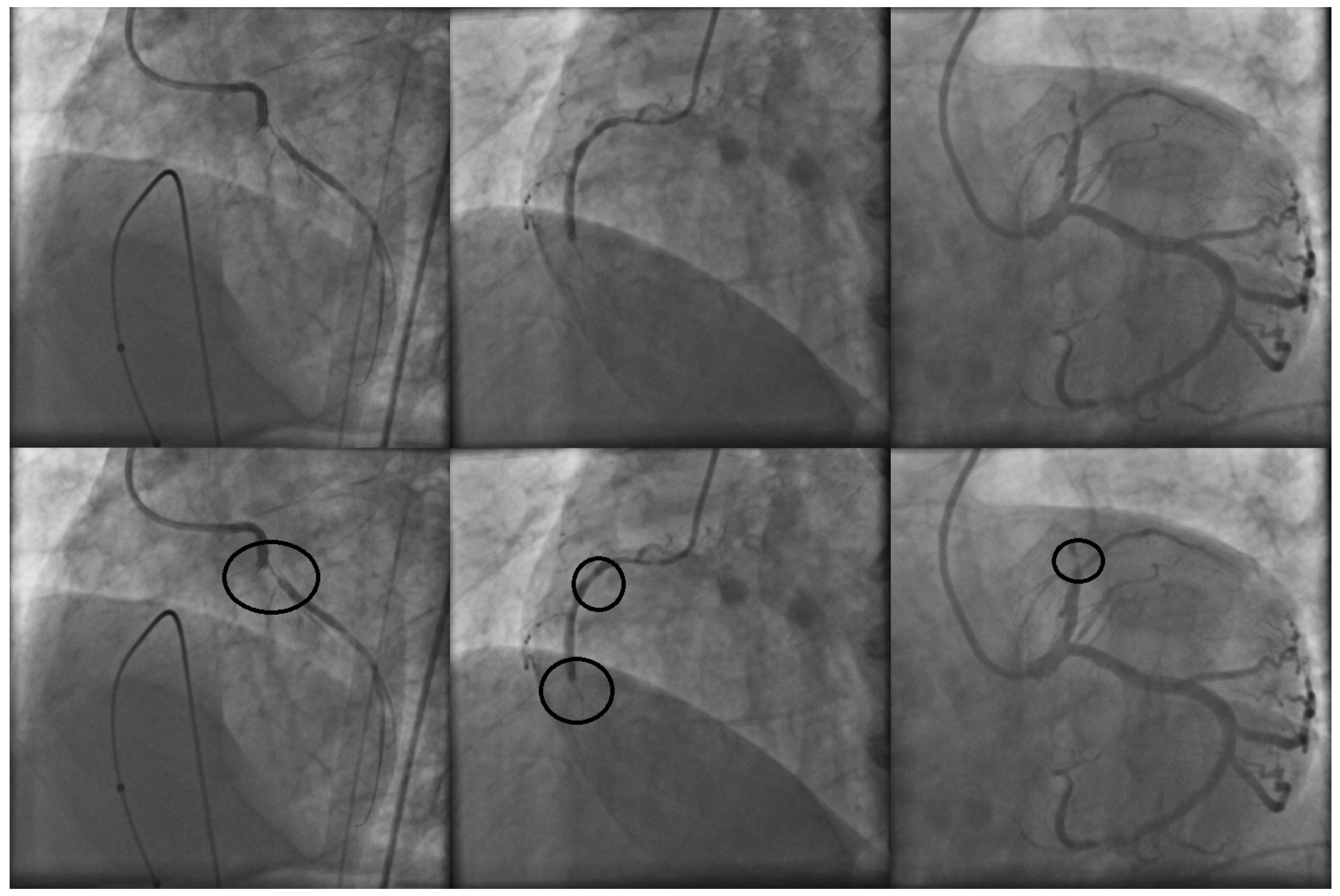Figure 1 illustrates a set of three X-ray coronary angiograms and the regions with stenosis that were labeled by the specialist.

Figure 1. X-ray coronary angiograms in the first row and their respective stenosis areas labeled by the specialist in the second row.

The automatic stenosis detection problem on coronary X-ray angiograms is a challenging task in computer aided diagnosis systems (CAD systems) because of the low contrast and the presence of high noise levels in almost all angiograms. This problem has been addressed using different techniques and strategies. Saad [1] used a vessel-width variation to determine the presence of atherosclerosis in a coronary artery image. The main drawback of this method relies on the need to have a high rate of accuracy on the vessel detection process in order to acquire a certain artery tree skeleton. The obtained skeleton is after used to determine the vessel centerline and compute the orthogonal line-length of a fixed-size window moving through the image. Kishore and Jayanthi [2] proposed a manually fixed-size window from an enhanced image. When the vessel pixels are determined, the width is measured adding intensity values from the left to right edge with no need of a skeletonization process.

The Hessian matrix properties have been also used to address the stenosis detection problem. Wan et al. [3] computed a vessel diameter estimation using a smoothed vessel centerline curve from the candidate stenosis regions detected by using the Hessian matrix. Sameh et al. [4] used the Hessian matrix to obtain a vessel-enhanced image in order to identify narrowed arteries regions. Cervantes-Sanchez et al. [5] computed the vessel-width by applying the second-order derivative over previously enhanced images. Using the local-minima approach, regions with a low-width measure are considered as stenosis candidates. Cruz-Aceves et al. [6] were able to design a Naive-Bayes classification method for stenosis detection using specific feature vectors and the second order derivative.

On the other hand, Convolutional Neural Networks (CNNs) are another approach used for image processing in order to detect specific features that are used to classify and discriminate elements in the original image [7]. They have proved to achieve good results in diverse application areas such as medical imaging processing, image enhancement, segmentation and classification [8]. One common approach related with CNNs is the use of pretrained neural networks in order to increase the accuracy rate while the training time is reduced significantly. This process is also known as transfer-learning [9,10,11]. In addition, the data augmentation technique is commonly used as a way to provide more data diversity to the CNNs [12,13,14]. Mikolajczyk and Grochowski [15] described some data augmentation methods and how they are used with transfer learning in order to improve the classification results obtained by CNNs in synthetic color transformations, malignant melanoma detection and face recognition. Moreover, Antczak and Liberadzki [16] proposed the use of CNNs for stenosis detection using data augmentation. They designed a model able to generate new random synthetic (positive and negative) stenosis patches based on a Gaussian kernel. Obtained results demonstrated how CNN efficiency is improved combining natural and synthetic cases.

Another of the explored approaches for image classification is related with the analysis of textures, feature extraction and feature selection. Frame et al. [17] used texture measures to find regions with retinopathy diseases in retinal images. Perez-Rovira et al. [18] introduced new measurable vessel features such as vessel tortuosity, branching coefficients and fractal analysis in order to quantify retinal vessel properties than can be used for image classification. Martinez-Perez et al. [19] used feature extraction techniques in order to measure and quantify geometrical and topological properties of continuous vessel trees in retinal images. Doukas et al. [20] designed an angiogenesis quantification model which is computed from a set of statistic measures that are obtained measuring features related with vessels length, density, contrast, entropy and branching points. Welikala et al. [21] proposed a method to detect proliferative diabetic retinopathy based in the extraction and selection of certain features that are able to achieve the highest accuracy rates. They started extracting a set of 21 different features. By applying a Genetic Algorithm (GA) for feature selection, they were able to acquire high accuracy rates detecting new retinopathy cases using a maximum subset of 9 features.

In the present work, a novel method for the automatic classification of stenosis cases in X-ray angiograms is proposed. The proposed method uses the machine learning technique of Support Vector Machine (SVM) for the classification of coronary stenosis. In literature other recent works using similar approaches have demonstrated the effectiveness of the SVM for classification tasks in medical images [22,23,24]. The proposed method starts by defining an initial set of 49 features related with pixel intensities, texture analysis and vessel morphology. On a second stage, an automated selection process supported by the Univariate Marginal Distribution Algorithm is performed. It is important to be mentioned that the use of metaheuristic strategies is highly recommended since the search space to find the most suitable combination of features (feature selection) is $2^{49}$, which is difficult to be examined in an exhaustive way using common hardware capabilities. The proposed method has several advantages over other techniques since it works with measurable image features instead of the image itself as in the case of CNNs, avoiding the complex configurations and tuning required to achieve a robust predictive model. The experimentation was performed using an image database with 500 image patches of coronary angiograms. To assure the results achieved by the SVM-based classification method and the subset of selected features, the Antczak image dataset [16] was used, probing that a machine learning technique plus a suitable feature set are able to overcome the results achieved by deep learning techniques. Another contribution of this paper is the identification of the most important features that lead to a correct classification of coronary stenosis.

The present paper is organized as follows. In Section 2 the underlying methods and techniques that were used and applied on this research are described in detail. Section 3 describes the proposed method including a detailed description of the used features and the evaluation metrics that were applied in order to assess the obtained results. In Section 4 the obtained results are presented and compared with different state-of-the-art methods. Finally, in Section 5 the concluding remarks are discussed.

2. Methodology

2.1. Feature Extraction

In digital image processing, the feature extraction concept refers to the multiple measure- ments and metrics that are possible to obtain from an image or a region on it. The measure- ments can be used to find patterns or values that are able to describe regions or objects in images. The most used strategy for feature extraction is the local image features (also known as interest points, key points and salient features). Local features can be defined as a specific pattern which is unique from its immediately close pixels, which are generally associated with one or more image properties [25,26]. Finding suitable feature descriptors is a challenging task because of the wide number of computer vision applications which require different features. This also includes the vast types of images and their associated issues such as illumination, resolution, contrast and noise levels. Many strategies and approaches to extract features are described in literature [27,28,29,30].

2.1.1. Texture Features

For texture analysis, the Gray-Level Co-Occurrence Matrix (GLCM) is widely used to extract texture features by considering spatial relationship between pixels [31]. The GLCM is a matrix whose rows and columns correspond to the pixel intensities of the image or a region of it. The matrix content is calculated based on the frequency of a pixel with value i that occurs in a specific spatial relationship (offset) denoted as $(\Delta x,\Delta y)$ to a pixel with value j. This operation can be expressed as follows:

$$C_{\Delta x,\Delta y}(i,j)={\displaystyle \sum _{x=1}^n}{\displaystyle \sum _{y=1}^m}\left\{\begin{array}{c}1,\mathrm{if}I(x,y)=i\mathrm{and}I(x+\Delta x,y+\Delta y)=j\hfill \\ 0,\mathrm{otherwise}\hfill \end{array}\right.,$$

(1)

where $C_{\Delta x,\Delta y}(i,j)$ is the frequency which two pixels with intensities i and j at an specific offset $(\Delta x,\Delta y)$ occur. n and m represents the height and width of the image, respectively. i and j are the pixel values. $I(x,y)$ and $I(x+\Delta x,y+\Delta y)$ are the pixel values in the image I at position $(x,y)$ and $(x+\Delta x,y+\Delta y)$, respectively.

The Radon Transform is a technique used in medical image processing [32]. It was applied to measure features related with body slices in a X-ray tomography along a determined number of angles [33]. Furthermore, it has been also applied for feature extraction [34,35,36]. The Radon Transform is the projection of the image intensity along with a radial line oriented at specific angle. The Radon Transform $R(\rho ,\theta )$ of a function $f(x,y)$ on the plane is defined as follows:

$$R(\rho ,\theta )={\int }_{-\infty }^{\infty }{\int }_{-\infty }^{\infty }f(x,y)\delta (\rho -x\cos \theta -y\sin \theta )dxdy,$$

(2)

where $\delta \left(r\right)$ is the Dirac delta function which is zero except when $r=0$ and $\delta (\rho -x\cos \theta -y\sin \theta )$ in the definition of Radon Transform forces the integration of $f(x,y)$ along the line $\rho -x\cos \theta -y\sin \theta =0$.

2.1.2. Shape Features

Shape features provide valuable information such as direction and tortuosity of a segment, density of interest-pixels, length of a segment and number of bifurcations, just to name a few. However, in almost all cases, shape-related features require a preprocessing step. In this research, a vessel enhancement step was performed applying the Frangi method [37], which makes use of the eigen-values obtained from the Hessian matrix. The Hessian matrix is the result of the second-order derivative of a Gaussian kernel that is convolved with the original image. The Gaussian kernel is as follows:

$$G(x,y)=-exp\left(-\frac{x^2+y^2}{2{\sigma }^2}\right),\parallel y\parallel <L/2,$$

(3)

where $\sigma$ is the spread of the Gaussian profile and L is the length of the vessel segment.

The resultant Hessian matrix is expressed as follows:

$$H=\left(\begin{array}{cc}{H}_{xx}& H_{xy}\\ H_{yx}& H_{yy}\end{array}\right),$$

(4)

where $H_{xx}$, $H_{xy}$, $H_{yx}$ and $H_{yy}$ are the different convolution responses of the original image with each second-order partial derivative of the Gaussian kernel.

The segmentation function defined by Frangi for 2D vessel detection is as follows:

$$f\left(x\right)=\left\{\begin{array}{cc}0\hfill & \mathrm{if}{\lambda }_2>0,\hfill \\ exp\left(-\frac{R_b^2}{2{\alpha }^2}\right)\left(1-exp\left(\frac{S^2}{2{\beta }^2}\right)\right)\hfill & \mathrm{elsewhere}.\hfill \end{array}\right.$$

(5)

The $\alpha$ parameter is used with $R_b$ to control the shape discrimination. The $\beta$ parameter is used by $S^2$ for noise elimination. $R_b$ and $S^2$ are calculated as follows:

$$R_b=\frac{|{\lambda }_1|}{|{\lambda }_2|},$$

(6)

$$S^2=\sqrt{{\lambda }_1^2+{\lambda }_2^2},$$

(7)

where ${\lambda }_1$ and ${\lambda }_2$ are the eigenvalues of Hessian matrix.

On the other hand, the Medial Axis Transform (MAT) is a method widely used to extract skeletons from shapes [38]. It is commonly implemented using the Voronoi method, expressed as follows:

$$R_k=\{x\in X|d(x,P_k)\le d(x,P_j)\mathrm{for}\mathrm{all}j\ne k\},$$

(8)

where $R_k$ is the Voronoi region associated with the site $P_k$ (a tuple of nonempty subsets in the space X), which contains the set with all points in X whose distance to $P_k$ is not greater than their distance to the other sites $P_j$. j is any index different from k. $d(x,P_k)$ is a closeness measure from point x to point $P_k$. The Euclidean distance is commonly used as a closeness measure and it is defined as follows:

$$D(p_1,p_2)=\sqrt{{(x_2-x_1)}^2+{(y_2-y_1)}^2}$$

(9)

where $D(p_1,p_2)$ is the distance between two points $p_1$ and $p_2$ defined by coordinates $(x_1,y_1)$ and $(x_2,y_2)$, respectively.

In the image processing area, there exists several features that can be computed from the information provided by an image, such as that presented above. However, in many cases, not all of them are useful when segmentation, detection or classification tasks are performed. Several techniques have been developed to address the problem of reducing irrelevant or dependent features. Feature selection (variable elimination) helps in understanding data, reducing the effect of curse of dimensionality and improving the classification performance [39].

2.2. Univariate Marginal Distribution Algorithm

The Univariate Marginal Distribution Algorithm (UMDA) is a metaheuristic from the family of Estimation of Distribution Algorithms similar to Genetic Algorithms (GA) [40]. Instead of the population recombination and mutation concepts, UMDA uses the frequency of components in a population of candidate solutions in the construction of new ones. Each individual in the population is composed by a bit-string and denoted as: $x_i=[x_{i,1},x_{i,2},\dots ,x_{i,D}]$ where each element $x_{i,j}$ is called a gene. An array of vectors $X=[x_1,x_2,\dots ,x_{n_{p}op}]$ is called a population. In UMDA, the population evolves on each generation (iteration) t and the current population is denoted as $X^t$. On each iteration UMDA samples a subset $n_{set}$ with the individuals representing the best solutions. With the $n_{set}$ sample a new population is created based on a probabilistic model using the genes in the individuals [41]. This iterative process ends when a stopping criterion is reached. Compared with other population-based techniques, UMDA only requires three parameters to operate: population size, stopping criterion and population selection ratio. This technique has obtained better performance compared to other metaheuristics in terms of speed, computational memory and accuracy of solutions. The pseudocode of UMDA is described below (Algorithm 1).

Algorithm 1: UMDA pseudocode

2.3. Support Vector Machines

Support Vector Machines (SVMs) are supervised learning models that were first designed for binary classification [42,43]. Since SVMs are a supervised-learning technique, they require a priori labeled training data. The main strength of this technique relies on the use of higher dimensional projection in which original data are represented [44]. For instance, if two groups in a 2-D dimensional space are not linearly separable, the SVM will map the data to a high dimensional space where the linear separation is possible to achieve. Figure 2 shows an example using synthetic data representation in order to illustrate how a SVM is able to perform a linear classification by projecting data to higher dimensional orders to overcome the linear separability issues presented in their original space.

Figure 2. SVM linear classification. The final result presented in (d) illustrates how the circle data group is above the plane formed by the SVM. On the other side, the square data group is below the plane. (a) Data distribution; (b) Linear separability issues; (c) Support Vectors; (d) SVM Linear Classification projecting data from ${\mathbb{R}}^2$ to ${\mathbb{R}}^3$.

The support vectors are data-points corresponding to the two classes that are lying in both sides of the hyperplane. They have influence over the position and orientation of the hyperplane. Under this assumption, the hyperplane depends only on the support vectors and not on any other observations.

The projection of the original training data in a space $\chi$ to a higher dimensional feature space $\mathcal{F}$ is performed via a Mercer kernel operator. For a given training data $x_1,\dots ,x_n$, that are vectors in some space $\chi \subseteq {\mathbb{R}}^d$, the support vectors can be considered as a set of classifiers expressed as follows [45]:

$$f\left(x\right)=\left({\displaystyle \sum _{i=1}^n}{\alpha }_{i}K(x_i,x)\right).$$

(10)

When K satisfies the Mercer condition [46] it can be expressed as follows:

$$K(u,v)=\Phi \left(u\right)·\Phi \left(v\right),$$

(11)

where $\Phi :\chi \to \mathcal{F}$ and “·” denotes an inner product. With this assumption, f can be rewritten as follows:

$$\begin{array}{c}f\left(x\right)=w·\Phi \left(x\right),\hfill \\ w={\displaystyle \sum _{i=1}^n}{\alpha }_i\Phi \left(x_i\right).\hfill \end{array}$$

(12)

3. Proposed Method for Stenosis Detection

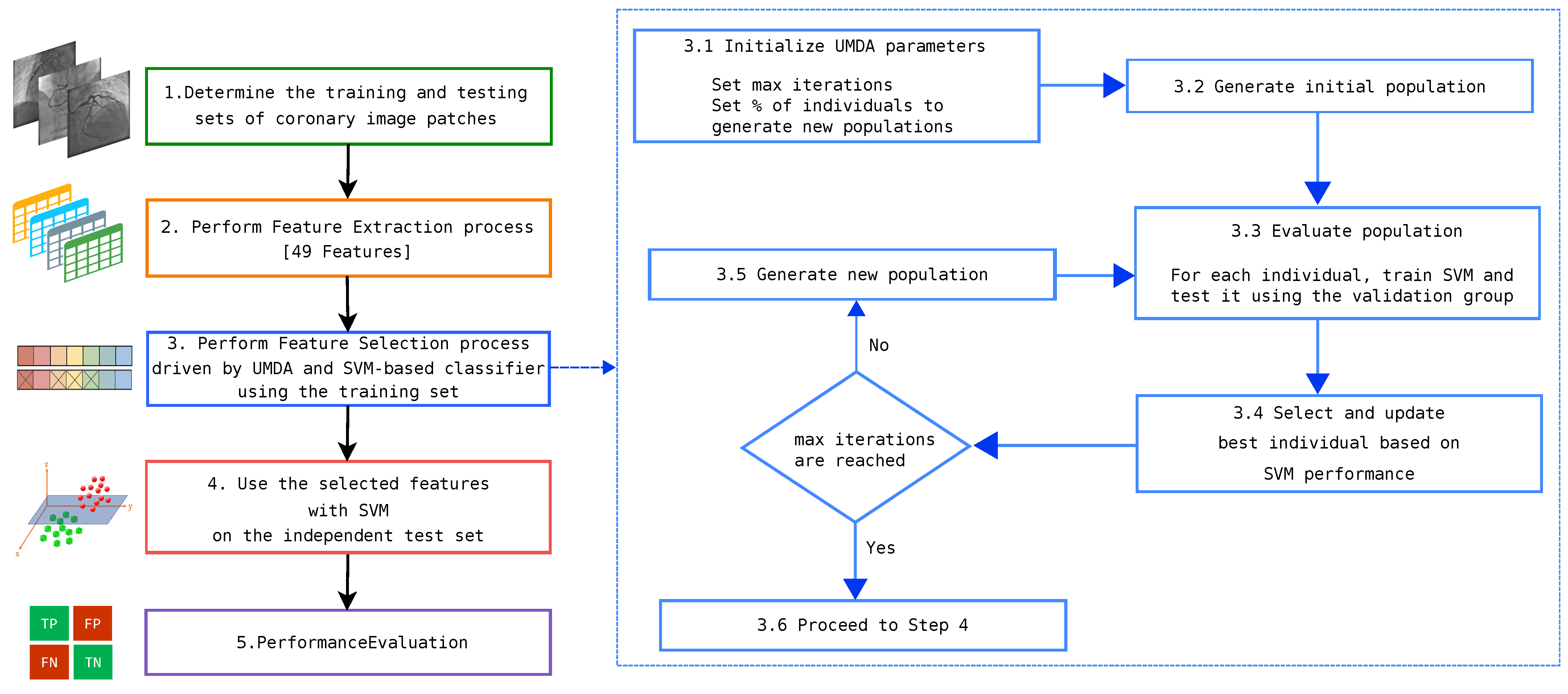
The proposed method is composed by several steps starting with the feature extraction task. This step transforms the X-ray images into a dataset formed by the defined features and their corresponding extracted values from each image patch. In the second step, a feature selection process is driven by UMDA, since the search space (the total number of combinations of selected and non-selected features) is $2^{49}$ computational complexity, which is not a suitable problem to be solved by an exhaustive strategy. In the final step, using the previously selected features, a SVM-based classifier is trained using the original feature dataset (removing unused features) and tested with new instances. The overall process is illustrated in Figure 3.

Figure 3. Flowchart of the proposed method for the automatic classification of coronary stenosis.

According to Figure 3, the process starts with a set of image patches that are extracted from coronary angiograms. The patch size must be enough to contain valuable information of vessels and positive stenosis cases. This step is commonly assessed by a cardiologist specialist. In addition, the rate of positive and negative cases must be similar.

Having the image patches bank, it is converted to a dataset by extracting features from patches. This task is referred to in literature as feature extraction. Feature types that can be extracted from images were described in the previous section. The feature set used in this paper is described in detail in the following subsection. It is important to be mentioned that some features require a previous image enhancement and segmentation in order to detect and skeletonize arteries. For vessel segmentation, the Frangi method was used. After applying the Frangi procedure, a new grayscale image was obtained containing enhanced vessel-like structures. However, an additional step is required in order to have a binary response that allows one to determine if each pixel corresponds to a vessel or background. In order to binarize the image, the Otsu method [47] was used since the binarization threshold is automatically calculated based on the pixel intensity in the image by computing the weighted sum of variance of two classes, expressed as follows:

$${\sigma }_{\omega }^2\left(t\right)={\omega }_0\left(t\right){\sigma }_0^2\left(t\right)+{\omega }_1\left(t\right){\sigma }_1^2\left(t\right),$$

(13)

where ${\omega }_0$ and ${\omega }_1$ weights are the probabilities of the two classes separated by a threshold t, and ${\sigma }_0^2$ and ${\sigma }_1^2$ are the statistical variances of ${\omega }_0$ and ${\omega }_1$, respectively.

3.1. Feature Set

The feature set is formed by 49 different features computed from the image patches. Texture features (1 to 14) were computed using the Haralik feature extraction method [31]. Basic pixel intensity features (features 15 to 18) and Shape-based Welikala features [21] (19 to 28) were also extracted, which required a previous segmentation and skeletonization procedure. The segmentation and skeletonization procedures were performed by using the Frangi and Medial-Axis Transform methods respectively. Statistic measures were also applied to the vessel shapes (features 29 to 31). For the rest of the features, the Radon Transform [34,48] was applied to each patch in order to obtain different projected intensity metrics (features 32 to 35). Finally, the Haralik texture features were extracted from the Radon Transform response of the patches (features 36 to 49). The full feature set is described as follows.

1–14.

Features 1 to 14 are composed by the Haralik features: angular second moment (energy), contrast, correlation, variance, inverse difference moment (homogeneity), sum average, sum variance, sum entropy, entropy, difference variance, difference entropy, information measure of correlation 1, information measure of correlation 2, maximum correlation coefficient.

15.

The minimum pixel intensity present in the patch.

16.

The maximum pixel intensity present in the patch.

17.

The mean pixel intensity in the patch.

18.

The standard deviation of the pixels intensities in the patch.

19.

The number of pixels corresponding to vessels in the patch.

20.

The number vessel segments in the patch.

21.

Vessel density. The proportion of vessel-pixels present in the patch.

22.

Tortuosity 1. The tortuosity of each segment was calculated using the true length (measured with the chain code) divided by the Euclidean length. The mean tortuosity was calculated from all the segments within the patch.

23.

Vessel Length.

24.

Number of bifurcation points. The number of biffurcation points within the sub window when vessel segments were extracted.

25.

Gray level coefficient of variation. The ratio of the standard deviation to the mean of the grey level of all segment pixels within the patch.

26.

Gradient mean. The mean gradient magnitude along all segment pixels within the sub window calculated using the Sobel gradient operator applied on the preprocessed image.

27.

Gradient coefficient of variation. The ratio of the standard deviation to the mean of the gradient of all segment pixels within the sub window.

28.

Mean vessel width. Skeletonization correlates to vessel center lines. The distance from the segment pixel to the closest boundary point of the vessel using the vessel map prior to skeletonization. This gives the half-width at that point which is then multiplied by 2 to achieve the full vessel width. The mean is calculated for all segment pixels within the sub window.

29.

The minimum standard deviation of the vessels length, based on the vessels present in the patch.

30.

The maximum standard deviation of the vessels length, based on the vessels present in the patch.

31.

The mean of the standard deviations of the vessels length, based on the vessels present in the patch.

32.

The Radon Ratio-X measure.

33.

The Radon Ratio-Y measure.

34.

The mean of the pixels intensities of the Radon Transform response of the patch.

35.

The standard deviation of the pixels intensities of the Radon Transform response of the patch.

36–49.

The Haralik features applied to the Radon Transform response of the patch: angular second moment (energy), contrast, correlation, variance, inverse difference moment (homogeneity), sum average, sum variance, sum entropy, entropy, difference variance, difference entropy, information measure of correlation 1, information measure of correlation 2, maximum correlation coefficient.

3.2. Evaluation Metrics

In order to evaluate and compare the performance of the different methods applied in this research, the Accuracy and Jaccard Index metrics have been adopted. The Accuracy (ACC) metric can be computed as follows:

$$ACC=\frac{TP+TN}{TP+TN+FP+FN},$$

(14)

where $TP$ is the number of positive instances that were labeled as positive by the classifier; $TN$ is the number of negative instances labeled as negative by the classifier; $FP$ is the number of negative instances labeled as positive by the classifier, and $FN$ is the number of positive instances labeled as negative by the classifier. In addition, the Jaccard Index or Jaccard Similarity Coefficient [49] measure was also used to assess the classification performance, which is calculated as follows:

$$Jaccard=\frac{TP}{TP+FP+FN}.$$

(15)

4. Results and Discussion

In this section, the experimental results using two different X-ray image databases are presented. The first database was provided by the Mexican Social Security Institute (IMSS) and approved by a local committee under reference R-2019-1001-078. It contains 180 digital images of coronary angiographies and their corresponding ground-truth outlined by an expert cardiologist. Each X-ray image is in gray-scale of size $512\times 512$ pixels. In total, a set of 500 patches of $64\times 64$ pixels was formed. Half of them were labeled as positive cases and the remaining instances were labeled as negative cases (image background or healthy arteries). The patch size and step were validated by the specialist based on the marks drawn of the areas with presence of possible stenosis cases in the ground-truth angiograms. For the training set, a subset of 400 patches was selected from the first database. Those instances were used in the feature selection stage. The remaining 150 instances were used for testing after the feature selection stage finished. The second image database was formed from the natural stenosis Antczak and Liberadzki dataset [16]. It contains 125 positive instances plus a random selection of 125 negative instances obtained from the same dataset. From the second database, which contains a total of 250 instances, 150 were used for the SVM training and the remaining 100 for testing. It is important to mention that the second database was not used in the feature selection stage. Furthermore, it was used as an independent test to assure the effectiveness of the previously selected features after the feature selection stage finished. All dataset groups were designed to have positive (stenosis) and negative (non-stenosis) instances in a rate of 50%–50%, respectively. Figure 4 illustrates samples of patches with positive and negative stenosis cases. The patches were extracted from the first image database. The first and second rows contain samples labeled as positive cases. The third and fourth rows present negative samples which contain healthy arteries and/or background.

Figure 4. Patch samples with positive stenosis cases (first and second rows) and negative cases (third and fourth rows).

All the computational experiments were implemented using the Matlab 2018a platform over an Intel i3 of 4th generation processor and 4 GB of RAM.

For the feature selection process, the following 5 metaheuristics of the state of the art were compared: Univariate Marginal Distribution Algorithm (UMDA) [40], Genetic Algorithm (GA) [50,51], Tabú Search (TS) [52], Iterated Local Search (ILS) [53] and Simulated Annealing (SA) [54]. The UMDA was experimentally set as population size of 30 individuals, 1500 iterations and selection rate of $0.70$. The GA was also experimentally configured with a population of 200 individuals, 1500 generations, crossover rate of $0.70$ and mutation probability of $0.01$. For the classification procedure, a Support Vector Machine was applied using a cross validation model with $k=10$ and $\mathit{maxiterations}=1000$.

In Table 1, the statistical comparison using 30 independent trials between the five metaheuristics is presented. Although the GA obtains competitive results, the UMDA method obtains the best performance in terms of the statistical measures, with the selection of 20 features. Based in this comparison, UMDA was selected for further analysis.

Table 1. Statistical analysis of the performance obtained for the feature selection task with 5 search strategies. The number of features corresponds to the number of features used in their best result.

Metaheuristic	Number of Features	Min	Max	Mean	Median	Std.Dev.
UMDA	20	0.9298	0.9497	0.9389	0.9393	0.0058
GA	19	0.9004	0.9303	0.9167	0.9208	0.0114
TS	35	0.8195	0.8713	0.8505	0.8596	0.0174
ILS	26	0.8575	0.9201	0.8938	0.8994	0.0198
SA	27	0.8596	0.9131	0.8819	0.8777	0.0148

In the previous analysis, significant results and findings were obtained by each metaheuristic, which offer a better understanding of the problem since they can be analyzed from a overall performance point of view and from a detailed analysis of the selected features obtained by the selection process. In Table 2, the most relevant features according to UMDA are illustrated.

Table 2. Selected Features obtained from the proposed method based on UMDA and the SVM using the training set of X-ray angiograms.

Feature Name	Frequency
Radon Ratio X	0.93
Radon Sum Variance	0.86
Number Of Vessel Segments	0.80
Number Of Bifurcation Points	0.70
Variance	0.70
Radon Entropy	0.66
Max Pixel Intensity	0.63
Vessel Std Dev Min	0.63
Radon Variance	0.60
Radon Maximal Correlation Coefficient	0.60
Radon Mean	0.56
Angular Second Moment (Energy)	0.50
Sum Entropy	0.50
Radon Ratio Y	0.46
Sum Average	0.46
Sum Variance	0.43
Tortuosity 1	0.43
Grey Level Coefficient Of Variation	0.43
Radon Information Measure Of Correlation 2	0.36
Radon Contrast	0.33

Based on the selected features presented in Table 2, it is important to point out that three of the most frequent features used by UMDA are related with texture measurement over the Radon Transform of the image. This can be explained because the linear projection of the image at determined angles leads to discover new texture features that are significant in classification tasks. In addition, other Radon Transform texture-based features were useful for the stenosis classification problem since they were also selected by UMDA. Morphological features such as number of vessel segments, tortuosity and number of bifurcation points allow the classifier to detect positive or negative stenosis cases. For the group of features related with pixel intensity, only the variance and the max intensity value were used for the classification task, discarding the rest of the features in this feature set.

In order to compare the performance of the proposed method, different classification methods of the state of the art were selected. The FeedForward Neural Network (FFNN) and BackPropagation Neural Network (BPNN) were experimentally configured with three hidden layers. Each hidden layer has 30 neurons when the input layer contains 49 neurons (the input features). Correspondingly, the hidden layers contain 12 neurons when input size have 20 neurons, keeping a fixed-ratio in hidden layer of $2/3$ of the input size [55]. The output layer contains 2 neurons: positive and negative case. The parameters used in all employed strategies were chosen by a trade-off between the required time to obtain a result and the Accuracy performance. For all machine learning techniques, the cross-validation technique was used in the training stage with $k=10$ from which 9 groups were used for training and 1 for validation. Additionally, three different deep learning architectures of convolutional neural networks (CNNs) were trained and tested using the corresponding original image patches (with size of $64\times 64$ pixels):

• The UNet, which is widely used for medical image classification [56]. The reference implementation was designed by Harouni [57].
• A convolutional neural network with 16 convolutional layers, designed by Antczac [16] for coronary stenosis classification.
• The GoogLeNet (GLNet), a fully-pretrained CNN with a large image database, implemented by [58].

All neural networks, including CNNs, were configured to have 1000 max epochs as a trade-off between Accuracy and required time to be trained. In Table 3 the performance results using the X-ray coronary stenosis database provided by the Mexican Social Security Institute (IMSS) are presented.

Table 3. Performance comparison of the proposed method using the database of the Mexican Social Security Institute (IMSS).

Method	Number of Features	Validation Accuracy	Accuracy	Jaccard Index
FFNN	20	0.81	0.78	0.66
	49	0.83	0.80	0.67
BPNN	20	0.82	0.79	0.66
	49	0.84	0.82	0.68
SVM	49	0.90	0.87	0.77
GLNet [58]	–	0.88	0.85	0.78
UNet [57]	–	0.91	0.87	0.79
CNN-16C [16]	–	0.91	0.86	0.79
Propossed Method	20	0.93	0.89	0.80

Table 4 presents the confusion matrix using the test set of the IMSS database obtained by the SVM classifier. The corresponding values were used to measure the Accuracy presented in Table 3.

Table 4. Confusion matrix of the results obtained by the SVM-based classifier using a set with 20 features along with the test set containing 100 instances from the first database (IMSS).

		Real Class
		Positive	Negative	Total
Predicted Class	Positive	44	5	49
	Negative	6	45	51
	Total	50	50	100

Table 5 presents the classification results using the publicly available Antczak’s X-ray image database.

Table 5. Performance comparison of the proposed method using the natural dataset from the Antczak’s image database.

Method	Number of Features	Validation Accuracy	Accuracy	Jaccard Index
FFNN	20	0.72	0.68	0.54
	49	0.68	0.67	0.61
BPNN	20	0.74	0.69	0.57
	49	0.71	0.71	0.60
SVM	49	0.78	0.70	0.61
GLNet [58]	–	0.77	0.72	0.63
UNet [57]	–	0.81	0.76	0.72
CNN-16C [16]	–	0.88	0.86	0.74
Proposed Method	20	0.92	0.88	0.79

By analyzing Table 3 and Table 5, the best performance on both test cases was achieved by the proposed method in terms of Accuracy and Jaccard Index. It can be observed that SVM performance is decreased when all the feature set is used in the classification process. This can be explained because of the high-dimensional complexity of the problem in which the hyperplane needs to be formed on a dimension greater to the 49-D, including a low data dispersion in some features which make difficult their linear separability. For this reason, when the number of dimensions was decreased and only a certain subset of them were used, the SVM-based classifier was able to achieve a high performance Accuracy and Jaccard Index rates, by using only 20 of the 49 features. However, for the FFNN and the BPNN techniques, the reduction of features has a negative effect on them, because of the loss of information when a non-lineal data separation is performed. Even when both machine learning techniques were trained with more instances, an over-fitting behavior occurred, classifying all instances in the test cases as positives or negatives depending also on which configuration was applied on the hidden layer. The CNN, U-Net and CNN-16 presented a good performance behavior. However, deep learning techniques work with the image itself rather than specific features. Finally, the Validation Accuracy performance is shown in column 3 of the corresponding tables, which was obtained in the training stage of each technique.

Table 6 presents the confusion matrix using the test set of the Antczak’s database obtained by the SVM classifier. The corresponding values were used to measure the Accuracy presented in Table 5.

Table 6. Confusion matrix of the results obtained by the SVM-based classifier using a set with 20 features along with the test set containing 100 instances from Antczak’s database.

		Real Class
		Positive	Negative	Total
Predicted Class	Positive	44	6	50
	Negative	6	44	50
	Total	50	50	100

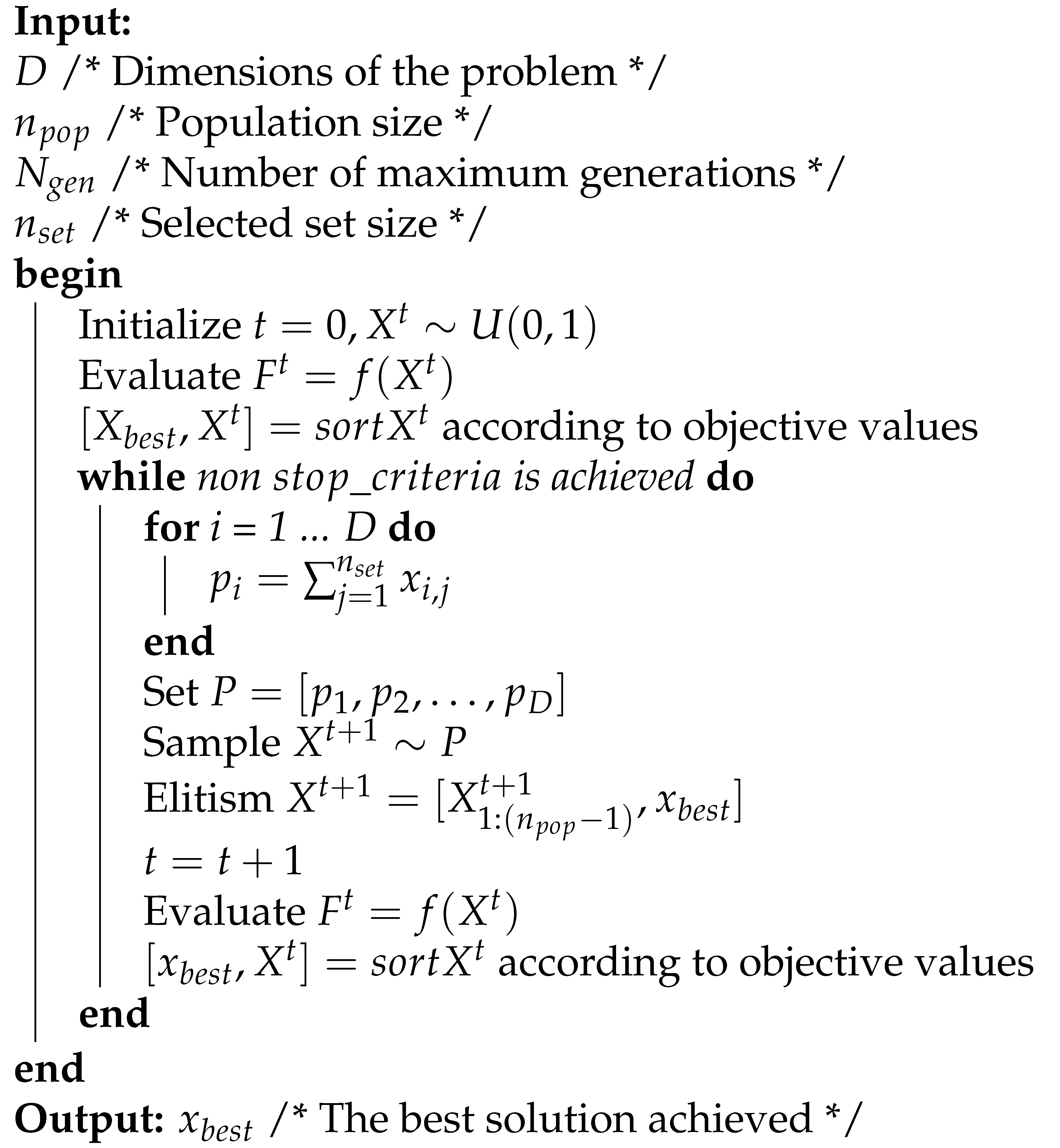
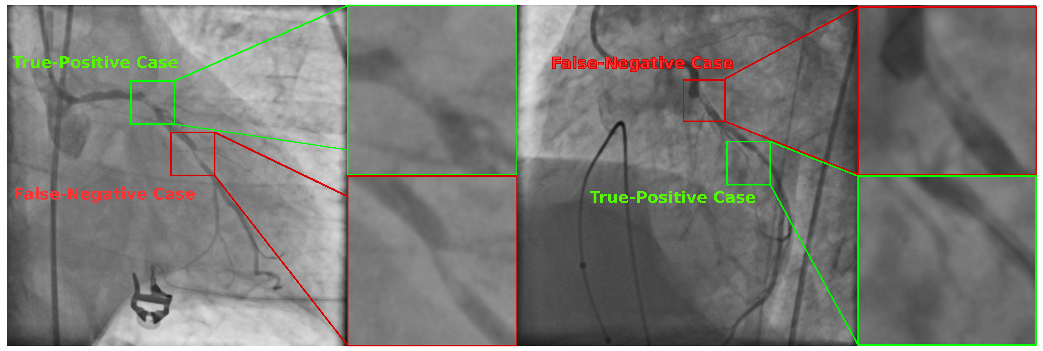
In order to illustrate the detection of coronary stenosis in X-ray images, Figure 5 illustrates two selected angiograms with certain zones classified as positive stenosis cases by the SVM-based classifier. However, only two of them were classified correctly. The other two instances are non-stenosis regions according to the specialist.

Figure 5. Selected X-ray angiograms with True-Positive and False-Positive stenosis cases detected by the SVM-based classifier using the set with 20 features found by UMDA.

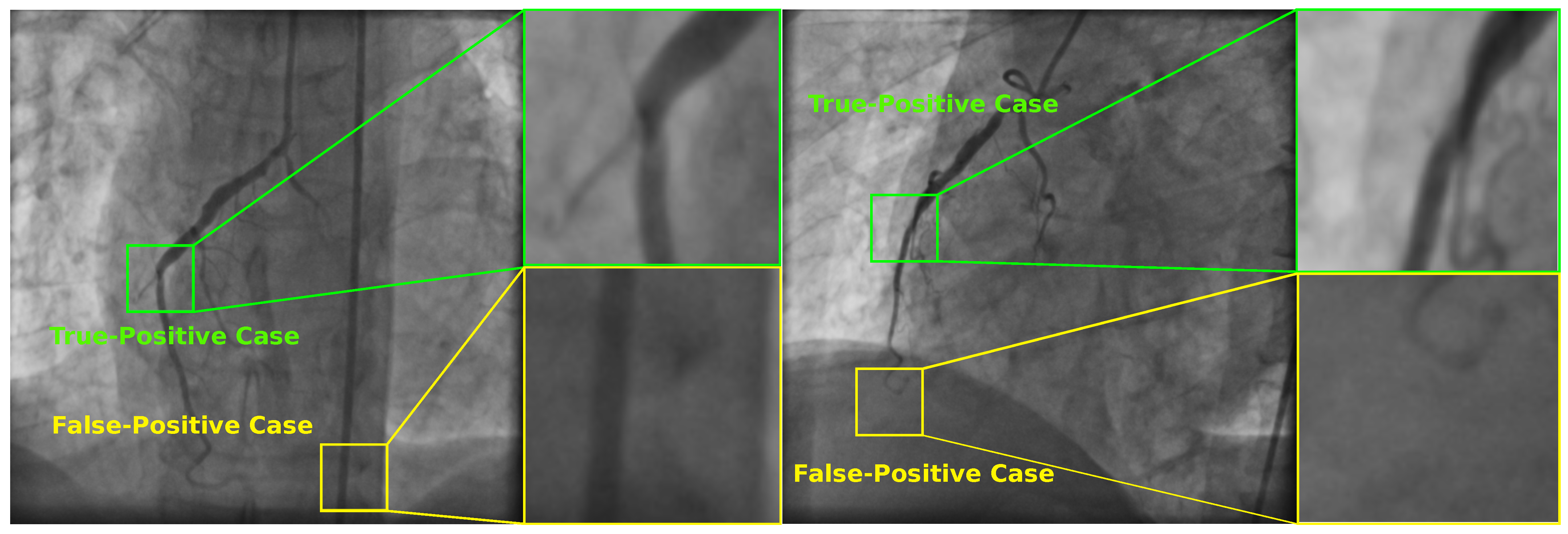
Figure 6 illustrates two selected angiograms which include correct and incorrect classification results. In the first scenario, the classifier failed to detect positive stenosis cases since it labeled regions as negative when there were present stenosis cases. The remaining labeled cases were classified in a correct way.

Figure 6. Selected X-ray angiograms with True-Positive and False-Negative stenosis cases detected by the SVM-based classifier using the set with 20 features found by UMDA.

Finally, in Table 7 is described the average time required by each method for their corresponding training and single-instance classification stages.

Table 7. Performance in terms of the mean time required by each classifier for training and single-instance classification, measured in seconds.

Method	Epochs/Max Iterations	Training Time	Classification Time
FFNN	1000	85	0.03
BPNN	1000	63	0.07
GLNet	1000	4500	6.47
UNet	1000	5500	5.45
CNN-16C	1000	3900	4.48
SVM	-	57	0.02
Proposed Method	-	42	0.02

5. Conclusions

In this paper, a novel method for automatic stenosis classification in X-ray coronary images based on feature selection has been introduced. The main contribution is the identification of a suitable subset of 20 features that allows one to classify stenosis cases in X-ray coronary images with a high performance overcoming different state-of-the-art classification techniques including deep learning strategies. The method consists of the three steps of feature extraction, feature selection and automatic classification. In the first stage, an initial set of 49 features was extracted from the entire image database. In the second stage, an automatic feature selection process was performed to address the high-dimensional optimization problem of $O\left(2^{49}\right)$ computational complexity. In this stage, five different metaheuristics were statistically compared in terms of the Accuracy and Jaccard Index using 30 trials. Furthermore, using only the 20 feature subset, the SVM-based classifier was able to improve the classification performance rather than using all the 49 feature set. As shown in experimental results, the classification performances in terms of the Accuracy and Jaccard Index metrics were $0.89$ and $0.80$ respectively, for the first image database. Moreover, when the same subset of 20 features was applied to the Antczak image database, the classification efficiency was higher than using deep learning techniques by achieving $0.88$ and $0.79$ for the Accuracy and Jaccard Index metrics, respectively. Another advantage with the proposed method is the fact of avoiding the use of data augmentation or other additional strategies to generate big training datasets. In addition, the classification efficiency and the average computational time (≈0.02 s) make it suitable to be applied in clinical practice. It was shown that having a suitable set of features, it is possible to classify coronary stenosis cases with a high efficiency. As future work a more robust evolutionary algorithm can be used to obtain a lower number of computational features while increasing the classification performance in an efficient computational time. In addition, according to the experimental results, the method is highly suitable to be considered as part of a computer-aided diagnosis system to assists cardiologists in the detection of coronary stenosis cases, which is helpful in angioplasty procedures and post-operative procedures.