Simulation of Heat and Water Transport on Different Tree Canopies: A Finite Element Approach

Abstract

Heat and water transport modeling is a widely explored topic in micro-meteorology, agriculture, and forestry. One of the most popular models is the Simultaneous Heat and Water (SHAW) model, which includes partial differential equations (PDEs) for air-soil temperature and humidity, but with a priori discretized PDE for the foliage temperature in each canopy layer; it is solved using the finite difference method and the canopy shape is defined as a simple rule of proportionality of total quantities such as the total leaf area index. This work proposes a novel canopy shape characterization based on Weibull distribution, providing a continuous vertical shape function capable of fitting any tree species. This allows formulating a fully continuous SHAW-derived model, which is numerically solved by a finite element approach of P₁ Lagrange type. For this novel approach, several numerical experiments were carried out to understand how the shape of well distinguishable canopies influences heat and water transport.

1. Introduction

Forest and plant canopies have vertically varying profiles of different physical quantities related to complex transport processes. Variables as leaf temperature, water potential, wind velocity, longwave and shortwave radiation, photosynthesis, air and soil temperatures, but also the fluxes between soil-canopy-air have vertical profiles which change in function of the vertical distribution of the canopy biomass—mainly its leaves—(see the review by [1] and references therein). Such variability of physical properties deeply affects evapotranspiration and heat fluxes within the soil-vegetation-atmosphere system (SVAT).

To study complex processes within the canopy, mathematical models with a single homogeneous biomass layer —the so-called “big leaf” models—were used as a first approach. Later models were improved by including soil-vegetation-atmosphere heat and mass fluxes, and finally, multi-layer models arise as a more realistic choice as the vertical canopy shape is considered. However, the multi-layer models sometimes are not necessarily better; thus, model selection is subject to the scope of study [1]. This allows the formulation of different models, single or multi-layered, to study the different phenomena in forest and plants canopies, some of which are harmful to human life quality. Several examples could be enunciated: an evaluation of the radiation that reaches the soil and tree transpiration as means to mitigate the urban heat island (UHI) [2], a study of trees resistance to wind loads, and efficiency evaluation of trees as windbreakers [3], formulation of a multi-layer model to estimate the radiation distribution inside the canopy [4], use of a high-resolution model to study the water stress in a forest mulch layering [5], estimation of heat and water fluxes in the soil layer [6].

One of the well-known models is the Simultaneous Heat and Water (SHAW) model formulated by Flerchinger et al. [7] as a PDEs’ model which has been updated several times [8,9,10], improving with it resolution associated with radiation, mass, sensible and latent heat fluxes, and recently [11] to model vertical profiles of temperature and humidity in a given tree canopy.

The SHAW model significantly depends on the leaf area index (LAI, a parameter that quantifies the canopy biomass) to model the leaf-air interchange of sensible heat and humidity. Frequently LAI is estimated merely as the total surface of leaves projected on a horizontal plane, known as total LAI, and holds no information about the vertical biomass distribution through the canopy [12]. The SHAW model requires a known value of LAI in each canopy layer, turning LAI in a priori discretized function; for example, in [11], this requirement is fulfilled with in situ measurements. This mandates a semi-discretized formulation of the SHAW model, leading to a finite difference scheme for its numerical resolution. Therefore, a continuous vertical function of LAI is needed for a continuous formulation of the SHAW model. The comments above lead us to focus on combining a continuous vertical canopy biomass profile with a multi-layer model to better approach vertical profiles of modeled state variables. As antecedents, in [13], the Weibull distribution is used successfully in curve fitting the leaf area density LAD—a vertical function of biomass canopy—of some tree species. On the other hand, in [14] a multi-layer, multi-species, and soil coupled model uses a continuous vertical function of LAD to upscale CO₂, water, heat, and momentum exchange from the canopy, validating the methodology with data from a tree canopy in Finland.

The accurate results shown in [14] suggest using a similar methodology to study —from a numerical point of view—the influence of the vertical canopy profile on the humidity and heat transport and air, leaf and soil temperatures. Therefore, in this paper, a SHAW-derived model is formulated in a fully continuous form (Section 2.1) using a continuous vertical profile of LAI drawn from the Weibull distribution (Section 2.2). After a detailed description of the initial and boundary conditions (Section 2.3), a combination of numerical techniques is proposed to solve the model (Section 2.4). It combines a finite element approach of $P_1$ Lagrange type for space discretization (a novelty in this kind of models), a finite difference scheme for time discretization, and a relaxed fix-point algorithm to address the resulting non-linear system. This method is applied in several numerical experiments where the resulting vertical profiles of leaf-air-soil temperatures, and humidity and heat fluxes corresponding to four different-shaped canopies showed notable variations (Section 3). Final remarks, discussions, and future work are presented in Section 4.

2. Materials and Methods

2.1. The Mathematical Model

In the model an air column with height $h_a$ has within a tree canopy with height $h_c$ and trunk height $h_0$ (then $0<h_0<h_c<h_a$). Furthermore, a soil layer with depth $h_s$ is considered. Then we define the following sub-domains, the air column ${\Omega }_a=(0,h_a)$, the foliage layer of the canopy ${\Omega }_c=(h_0,h_c)$ and the soil layer ${\Omega }_s=(0,h_s)$. All of them are such that ${\Omega }_c\subset {\Omega }_a$ and ${\Omega }_s\cap {\Omega }_a=\varnothing$.

Now, we look for the state functions of air temperature $T_a(z,t)$, air humidity $p_v(z,t)$, leaf temperature $T_l(z,t)$, and soil temperature $T_s(z,t)$ such that satisfies the following nonlinear system of PDEs

$$\begin{array}{c}\hfill {\rho }_a{c}_a{\partial }_t{T}_a={\partial }_z[{\rho }_a{c}_a{K}_e{\partial }_z{T}_a+H_l(T_a,T_l)]\mathrm{on}{\Omega }_a\times [0,T]\end{array}$$

(1a)

$$\begin{array}{c}\hfill {\partial }_t{p}_v={\partial }_z[K_e{\partial }_z{p}_v+E_l(p_v,T_l)]\mathrm{on}{\Omega }_a\times [0,T]\end{array}$$

(1b)

$$\begin{array}{c}\hfill m_c{c}_c{\partial }_z{T}_l=S_n+L_n-H_l(T_a,T_l)-L_v{E}_l(p_v,T_l)\mathrm{on}{\Omega }_c\times [0,T]\end{array}$$

(1c)

$$\begin{array}{c}\hfill {\rho }_s{c}_s{\partial }_t{T}_s={\partial }_z\left({\lambda }_s{\partial }_z{T}_s\right)\mathrm{on}{\Omega }_s\times [0,T]\end{array}$$

(1d)

The mathematical model (1a)–(1d) is similar to the called Simultaneous Heat and Water (SHAW) model proposed by Flerchinger et al. [7,8] but not include a PDE related to soil humidity and Equation (1c) is continuous instead of discrete. The system incorporates air-canopy interchanges of sensible heat and humidity, absorbed shortwave and longwave net radiations, and assumes a well-mixed air column by turbulent transport. Consequently, the model needs complex empirical formulas, nonlinear coefficients, and correlations to define interchanges rates, resistances, friction velocity, and vertical wind profile. All of them are written down below as they were formulated in [7,8,11,15].

The turbulent transport coefficient $K_e$ is given by the widely use K-theory

$$K_e=\left\{\begin{array}{cc}k{u}_{\ast }(z-d+z_H)/{\varphi }_H\hfill & z>d\hfill \\ k{u}_{\ast }{z}_H/{\varphi }_H\hfill & z\le d\hfill \end{array}\right.$$

(2)

being k the Von Karman constant, $z_H$ the canopy height, $d\approx 0.77h_c$ the zero-level displacement, ${\varphi }_H$ is the dimensionless heat stability factor, and $u_{\ast }$ the friction velocity given by

$$u_{\ast }=u_{ref}k{\left[ln\left(\frac{z_{ref}-d}{z_m}\right)+{\psi }_m\right]}^{-1}$$

(3)

where $u_{ref}$ is the reference wind speed at a given height $z_{ref}$.

This formulations of $K_e$ and $u^{\ast }$ are simple and commonly accepted in Micrometerology but has limitations. It draws constant transport coefficients below the zero displacement height d; the stability factor ${\varphi }_H$ is calculated by sensible heat fluxes above the canopy; the effect of a sparse canopy and beyond the canopy could generate an undesirable damping effect [16,17]. Alternatives to address those limitations could be a non-parabolic approach for the free-surface layer given by a semi-theoretical coefficient of exponential type [17], the extended K-theory [18] or the called L-theory based on a Lagrangian point view of transport [16].

The interchange of sensible heat $H_l$ and humidity $E_l$ between air and canopy depends on the amount of foliage quantified by the leaf index area ($LAI$) as a vertical profile of the foliage mass, which will be defined later,

$$\begin{array}{c}\hfill H_l=2{\rho }_a{c}_{a}LAI\frac{T_l-T_a}{r_h}\end{array}$$

(4a)

$$\begin{array}{c}\hfill E_l=\left\{\begin{array}{cc}LAI\frac{p_{vs}-p_v}{r_{ls}+r_v}\hfill & p_{vs}\ge p_v\hfill \\ 0\hfill & p_{vs}<p_v\hfill \end{array}\right.\end{array}$$

(4b)

The ideal gas law is used to estimate the humidity in the leaf stomata $p_{vs}$ as a function of $T_l$,

$$p_{vs}=\frac{M_v}{R{T}_l}{e}_s\left(T_l\right)$$

(5)

where in turn $M_v$ is the molecular mass of water, R the universal gas constant, and $e_s\left(T_l\right)$ is the water vapor pressure. Meanwhile, the interchange resistances to convective heat between air and leaf $r_h$, humidity between air and leaf $r_v$, and the evaporation in the leaf stomata $r_{ls}$, are all defined as

$$\begin{array}{c}\hfill r_h=7.4\frac{{\rho }_a}{M_a}\sqrt{\frac{d_l}{u}}=7.4\frac{P}{R{T}_a}\sqrt{\frac{d_l}{u}}\end{array}$$

(6a)

$$\begin{array}{c}\hfill r_v=6.8\frac{{\rho }_a}{M_a}\sqrt{\frac{d_l}{u}}=6.8\frac{P}{R{T}_a}\sqrt{\frac{d_l}{u}}\end{array}$$

(6b)

$$\begin{array}{c}\hfill r_{ls}=\frac{r_{ls0}}{f_{S_t}{f}_T{f}_{VPD}}\left[1+{\left(\frac{{\mathsf{\Psi }}_l}{{\mathsf{\Psi }}_c}\right)}^{n_s}\right]\end{array}$$

(6c)

being u the wind profile, $d_l$ the leaf characteristic length, P the atmospheric pressure, $r_{ls0}$ the unstressed leaf interchange, ${\mathsf{\Psi }}_l$ the leaf water potential, ${\mathsf{\Psi }}_c$ the leaf critical water potential, and $f_{St},f_T,f_{VPD}$ are corrections on the stomata resistance to solar radiation, temperature and water vapor deficit, respectively. The wind profile has a logarithm profile above the canopy but exponentially decline in its interior

$$u=\left\{\begin{array}{cc}\frac{u_{\ast }}{k}\left[ln\left(\frac{z-d}{z_m}\right)+{\psi }_m\right]\hfill & z\ge h_c\hfill \\ \frac{u_{\ast }}{k}\left[ln\left(\frac{h_c-d}{z_m}\right)+{\psi }_m\right]exp\left(0.28{\left(\frac{LA{I}_{tot}^2{h}_c}{w_l}\right)}^{1/3}\left(\frac{z}{hc}-1\right)\right)\hfill & z<h_c\hfill \end{array}\right.$$

(7)

being $u_{\ast }$ the friction velocity, $z_m$ is the momentum transfer roughness, ${\psi }_m$ is the diabatic momentum stability factor, $w_l$ is the mean leaf width and $LA{I}_{tot}$ is the total Leaf Area Index of the canopy. Again, the velocity profile (7) is classical and agree with the comments to Equation (2); there are alternatives, for example, in the free-surface beyond the canopy $z>h_c$, a non-parabolic profile proposed recently in [17].

Other relations needed for computing parameters related to atmospheric stability are:

$$\begin{array}{c}\hfill {\psi }_H=\left\{\begin{array}{cc}{\displaystyle 4.7\zeta }\hfill & \zeta \ge 0\hfill \\ {\displaystyle -2ln\left(\frac{1+\sqrt{1-16\zeta }}{2}\right)}\hfill & \zeta <0\hfill \end{array}\right.\end{array}$$

(8a)

$$\begin{array}{c}\hfill {\varphi }_H=\left\{\begin{array}{cc}{(1-16\zeta )}^{-1/2}\hfill & \zeta \ge 0\hfill \\ 1+\frac{6\zeta }{1+\zeta }\hfill & \zeta <0\hfill \end{array}\right.\end{array}$$

(8b)

being the atmospheric stability $\zeta$ given by

$$\zeta =\frac{k{z}_{ref}g{H}_{\zeta }}{{\rho }_a{c}_a{T}_a{u}_{\ast }^3}$$

(9)

with the total exchange of sensible heat formulated as

$$H_{\zeta }=\frac{k^2{\rho }_a{c}_{a}u\left(z\right)[T_a(d+z_H)-T_a\left(z\right)]}{\left[ln\left(\frac{z-d}{z_m}\right)+{\psi }_m\right]\left[ln\left(\frac{z-d}{z_H}\right)+{\psi }_H\right]}$$

(10)

where ${\psi }_m=0.6{\psi }_H$ for unstable conditions and ${\psi }_m={\psi }_H$ for stable conditions.

Finally, $L_n$ and $S_n$ in (1c) represent the net longwave and shortwave radiations absorbed within the canopy, computed with a multi-layer model [4,9,15,19] (see Appendix A). To understand the effect of the canopy shape in the models’ state variables, ideal conditions must be considered. Therefore, the soil layer has a water concentration constant along time, justifying eliminate the PDE related to soil humidity in the model. Moreover, the water vapor on leaf stomata is assumed to be saturated, implying that Equation (5) holds.

2.2. The Weibull Distribution and Canopy Shape Characterization

In the above subsection, the vertical interchange of heat and humidity between air and canopy depends on the amount of foliage quantified by $LAI$ and —implicitly— of the foliage mass $m_c$. However, $LAI$ and $m_c$ are reported in field measurements as a 2D-flat projection, which in this work are called total leaf area index $LA{I}_{tot}$ and total canopy biomass $m_{c,tot}$, respectively. So a vertical parametrization of both $LAI$ and $m_c$ is needed. Therefore this subsection defines them as the most straightforward continuous vertical functions using the well-known Weibull distribution, being so one of the main contributions of this work.

The Weibull distribution is a two-parameter distribution used widely in biology, meteorology, sciences materials, and others. It can be described by its probability density function $f\left(v\right)$ and its cumulative distribution function $F\left(v\right)$ as described in [20]:

$$\begin{array}{c}\hfill f\left(v\right)=\frac{\beta }{\alpha }{\left(\frac{v}{\alpha }\right)}^{\beta -1}exp\left(-{\left(\frac{v}{c}\right)}^{\beta }\right)\end{array}$$

(11a)

$$\begin{array}{c}\hfill F\left(v\right)=1-exp\left(-{\left(\frac{v}{c}\right)}^{\beta }\right)\end{array}$$

(11b)

where $\beta$ is the Weibull module, $\alpha$ is the scale parameter and v is the independent variable. Is very important to note that $f\left(v\right)$ is the anti-derivative of $F\left(v\right)$ ($f\left(v\right)=F^{\prime }\left(v\right)$). Applying these concepts to the tree canopy, another element to consider is the called leaf area density $LAD=LAD\left(z\right)$, a vertical shape function that quantified mass change concerning the canopy height. Assuming that $LAD\left(z\right)$ is known, we can relate it with different $LAI$ definitions (see [13])

$$\begin{array}{c}\hfill LA{I}_{tot}=\underset{0}{\overset{h_c}{\int }}LAD\left(z\right)dz\end{array}$$

(12a)

$$\begin{array}{c}\hfill LA{I}_a=\underset{z}{\overset{h_c}{\int }}LAD\left(s\right)ds\end{array}$$

(12b)

being $LA{I}_a$ the cumulative leaf area index. The shape function $LAD\left(z\right)$ can be adjusted by the following Weibulls’ probability distribution [14,21,22]

$$LAD=LA{I}_{tot}\left(\frac{{\beta }_c}{{\alpha }_c}{\left(\frac{1-z/h_c}{{\alpha }_c}\right)}^{{\beta }_c-1}exp\left(-{\left(\frac{1-z/h_c}{{\alpha }_c}\right)}^{{\beta }_c}\right)\right)$$

(13)

Similarly, the cumulative $LA{I}_a$ is defined as the following Weibulls’ cumulative distribution

$$LA{I}_a=LA{I}_{tot}\left\{1-exp\left[-{\left(\frac{1-z/h_c}{{\alpha }_c}\right)}^{{\beta }_c}\right]\right\}$$

(14)

where in both cases $LA{I}_{tot}$ is taken as a proportionality constant. Defining $v=1-z/h_c$, we have that $LAD\left(v\right)=LA{I}_a^{\prime }\left(v\right)$ holds, and $LAI$ is computed straightforwardly in an arbitrary canopy layer of length $v_1-v_0$ in the following way

$$LAI=\underset{v_0}{\overset{v_1}{\int }}LAD\left(v\right)dv=LA{I}_a\left(v_1\right)-LA{I}_a\left(v_0\right)$$

(15)

taking $v_1=1-(z+\Delta z)/h_c$ and $v_0=1-z/h_c$ as relative positions in the plant canopy, an useful expression of $LAI$ in a canopy layer of length $\Delta z$ is formulated as

$$LAI\left(z\right)=LA{I}_{tot}\left(exp\left(-{\left(\frac{1-z/h_c}{{\alpha }_c}\right)}^{{\beta }_c}\right)-exp\left(-{\left(\frac{1-(z+\Delta z)/h_c}{{\alpha }_c}\right)}^{{\beta }_c}\right)\right)$$

(16)

In a totally similar way, the biomass of the foliage $m_c$ as a function of z could be formulated as

$$m_c\left(z\right)=m_{tot}\left(exp\left(-{\left(\frac{1-z/h_c}{{\alpha }_c}\right)}^{{\beta }_c}\right)-exp\left(-{\left(\frac{1-(z+\Delta z)/h_c}{{\alpha }_c}\right)}^{{\beta }_c}\right)\right)$$

(17)

being $m_{tot}$ the total biomass in the canopy.

2.3. Initial and Boundary Conditions

In this subsection, the initial boundary conditions will be formulated. For this purpose, it must be noted that the model domain has three physical borders: soil ($z=h_s$), interface soil-air ($z=0$) and air column height ($z=h_a$). There are no boundaries between the canopy and air; instead, there are interchanges of heat and water, which can be computed using the continuous function $LAI$ (Equation (16)). Therefore, assuming that in an initial time the air temperature, leaf temperature, humidity and soil temperature are known the following initial conditions are imposed to the state variables of the model $T_a(.,0)=T_a^0(.),p_v(.,0)=p_v^0(.),T_l(.,0)=T_l^0(.)$ and $T_s(.,0)=T_s^0(.)$. Concerning the boundary conditions, a heat and humidity flux is assumed in the upper part of the air column ($z=h_a$), and the same in the lower part of the soil layer ($z=h_s$). Then, with knowing reference time functions $T_{a,ref}\left(t\right)$, $p_{v,ref}\left(t\right)$ and $T_{s,ref}\left(t\right)$, the following boundary conditions are imposed for all $t\ge 0$

$$\begin{array}{c}\hfill {\rho }_a{c}_a{K}_e{\partial }_z{T}_a(h_a,t)=k_a(T_{a,ref}\left(t\right)-T_a(h_a,t))\end{array}$$

(18a)

$$\begin{array}{c}\hfill K_e{\partial }_z{p}_v(h_a,t)=k_v(p_{v,ref}\left(t\right)-p_v(h_a,t))\end{array}$$

(18b)

$$\begin{array}{c}\hfill \lambda {\partial }_z{T}_s(h_s,t)=k_s(T_{s,ref}\left(t\right)-T_s(h_s,t))\end{array}$$

(18c)

observing that for large value of the interchanges resistances $k_a,k_v,k_s\to \infty$, the previous conditions are transformed into the Dirichlet type conditions $T_a(h_a,t)=T_{a,ref}\left(t\right),p_v(h_a,t)=p_{v,ref}\left(t\right)$ and $T_s(h_s,t)=T_{s,ref}\left(t\right)$.

Finally, in the border between the soil layer and the air column ($z=0$), interchange of heat and water and soil heat balance are considered. Therefore we impose the following conditions,

$$\begin{array}{c}\hfill {\rho }_a{c}_a{K}_e{\partial }_z{T}_a(0,t)=-H_g(T_a,T_s)\end{array}$$

(19a)

$$\begin{array}{c}\hfill K_e{\partial }_z{p}_v(0,t)=-E_g(p_v,T_s)\end{array}$$

(19b)

$$\begin{array}{c}\hfill {\lambda }_s{\partial }_z{T}_s(0,t)=S_{n,0}+L_{n,0}-H_g(T_a,T_s)-L_v{E}_g(p_v,T_s)\end{array}$$

(19c)

where $H_g$ and $E_g$ are sensible heat and vaporization fluxes between air and soil, $L_v$ is the heat of vaporization, $S_{n,0}$ and $L_{n,0}$ are the net shortwave and longwave radiation absorbed by the soil. These last quantities must consider the process, which begins when the radiation reaches the upper part of the canopy and downward until reaching the soil. Therefore, a multi-layer model is used to approach them (see Appendix A). To compute the air-soil fluxes $H_g$ and $E_g$ similar formulations those above (in the canopy) are used, then

$$\begin{array}{c}\hfill H_g={\rho }_a{c}_a{\left.\frac{\left(T_s-T_a\right)}{r_s}\right|}_{z=0}\end{array}$$

(20a)

$$\begin{array}{c}\hfill E_g=\left\{\begin{array}{cc}{\displaystyle {\left.\frac{\left(p_{vg}-p_v\right)}{r_s}\right|}_{z=0}}& p_{vg}\ge p_v\hfill \\ 0& p_{vg}<p_v\hfill \end{array}\right.\end{array}$$

(20b)

where in turn $p_{vg}$ is the water steam concentration in the soil surface and $r_s$ is the soil resistance to convection [16], computed both by the following equations

$$\begin{array}{c}\hfill p_{vg}={\left.\frac{M_v}{R{T}_s}{e}_s\left(T_s\right)\right|}_{z=0}\end{array}$$

(21a)

$$\begin{array}{c}\hfill r_s=\frac{1}{u_{\ast }k}\left[ln\left(\frac{z_{ref,s}-d_s+z_{H,s}}{z_{H,s}}\right)+{\psi }_H\right]\end{array}$$

(21b)

where $z_{ref,s}$, $d_s$, $z_{H,s}$ are the reference height, zero displacement height and heat transfer roughness. As before, there are alternatives to the logarithm profile to estimate $r_s$, for example, which is derived from the extended K-Theory and introduced in [23].

2.4. Numerical Solution

2.4.1. Finite Element Approach

On the part of Equations (1a), (1b), (1d) the usual finite element treatment will be applied (see [24,25]); however, it must be observed that Equation (1c) has no spatial gradient, so requires an accurate time discretization instead, using finite differences [26]. To avoid tedious calculations and large formulations, a straightforward process is displayed in this subsection. Let the Sobolev spaces $V=H^1\left({\Omega }_a\right)$ and $W=H^1\left({\Omega }_s\right)$ and its $L^2(\Omega )$ inner product denoted by $⟨.,.⟩$. Furthermore, the spacial domain ${\Omega }_a\cup {\Omega }_s$ is meshed using two meshes ${\tau }_a$ and ${\tau }_s$, given by the partitions $h_a=z_{n_a}>z_{n_a-1}>\cdots >z_0=0$ and $0={\widehat{z}}_0>{\widehat{z}}_1>\cdots >{\widehat{z}}_{n_s}=h_s$ with $n_a+1$ and $n_s+1$ nodes respectively. It is important consider the existence of a canopy mesh ${\tau }_c$ with $n_c+1$ nodes covering the foliage layer ${\Omega }_c=(h_0,h_c)$ and such that ${\tau }_c\subset {\tau }_a$. Once the meshes are defined let be the discrete spaces $V_h=\{{\phi }_h\in C\left({\overline{\Omega }}_a\right):{\phi }_h{|}_{I_i}\in P_1\left(I_i\right)\}$ and $W_h=\{{\widehat{\phi }}_h\in C\left({\overline{\Omega }}_s\right):{\widehat{\phi }}_h{|}_{{\widehat{I}}_i}\in P_1\left({\widehat{I}}_i\right)\}$ such that $V\approx V_h$ and $W\approx W_h$, then it is possible formulate the following semi-discrete problem: Find $(T_a,p_v,T_l,T_s)\in V_h\times V_h\times V_h\times W_h$ and $T_l\in \mathcal{C}\left({\Omega }_c\right)$ such that for ${\phi }_i\in V_h$ and ${\widehat{\phi }}_m\in W_h$ satisfies the following system equations

$$\begin{array}{c}\hfill ⟨{\rho }_a{c}_a{\partial }_t{T}_a,{\phi }_i⟩+⟨{\rho }_a{c}_a{K}_e{\partial }_z{T}_a,{\phi }_i^{\prime }⟩+k_a{T}_a(h_a,t){\phi }_i\left(h_a\right)+k_{a0}{T}_a(0,t){\phi }_i\left(0\right)\\ \hfill =⟨{\partial }_z{H}_l,{\phi }_i⟩+k_a{T}_{a,ref}{\phi }_i\left(h_a\right)+k_{a0}{T}_s(0,t){\phi }_i\left(0\right)\end{array}$$

(22a)

$$\begin{array}{c}\hfill ⟨{\partial }_t{p}_v,{\phi }_i⟩+⟨K_e{\partial }_z{p}_v,{\phi }_i^{\prime }⟩+k_v{p}_v(h_a,t){\phi }_i\left(h_a\right)+k_{v0}{p}_v(0,t){\phi }_i\left(0\right)\\ \hfill =⟨{\partial }_z{E}_l,{\phi }_i⟩+k_v{p}_{v,ref}{\phi }_i\left(h_a\right)+k_{v0}{p}_{vg}(0,t){\phi }_i\left(0\right)\end{array}$$

(22b)

$$\begin{array}{c}\hfill m_c{C}_c{\partial }_t{T}_l=S_n+L_n-H_l-L_v{E}_l\end{array}$$

(22c)

$$\begin{array}{c}\hfill ⟨{\rho }_s{C}_s{\partial }_t{T}_s,{\widehat{\phi }}_j⟩+⟨{\lambda }_s{\partial }_z{T}_s,{\partial }_z{\widehat{\phi }}_j⟩-k_s{T}_s(h_s,t){\widehat{\phi }}_j\left(h_s\right)\\ \hfill =(S_{n,0}+L_{n,0}-H_g-L_v{E}_g){\widehat{\phi }}_j\left(0\right)-k_s{T}_{s,ref}{\widehat{\phi }}_j\left(h_s\right)\end{array}$$

(22d)

for each $i=0,\dots ,n_a;j=0,\dots ,n_s$ and being $k_{a0}=\frac{{\rho }_a{c}_a}{r_s}$, $k_{v0}=\frac{1}{r_s}$. Using the function basis for $V_h$ and $W_h$ is it possible to define over ${\tau }_a$ and ${\tau }_s$ the functions $T_a,p_v,T_s,T_l$ as the following lineal combination

$$\mathsf{\Phi }(z,t)=\sum _{j=0}^{n_x}{\xi }_j\left(t\right){\widehat{\mathsf{\Phi }}}_j\left(z\right)$$

(23)

being ${\xi }_j\left(t\right)=\mathsf{\Phi }(z_j,t)$ the time depend state variable and ${\left\{{\widehat{\mathsf{\Phi }}}_j\left(z\right)\right\}}_{j=0}^{n_x}$ the set of nodal basis functions. Thus, we define the following spacial discretized functions ${\mathbf{T}}_{\mathbf{a}}\left(t\right)={\left\{{\tilde{T}}_{a,j}\left(t\right)\right\}}_{j=1}^{n_a}$, ${\mathbf{p}}_{\mathbf{v}}\left(t\right)={\left\{{\tilde{p}}_{v,j}\left(t\right)\right\}}_{j=1}^{n_s}$, ${\mathbf{T}}_{\mathbf{s}}\left(t\right)={\left\{{\tilde{T}}_{s,k}\left(t\right)\right\}}_{k=1}^{n_s}$, and ${\mathbf{T}}_{\mathbf{l}}\left(t\right)={\left\{{\tilde{T}}_{l,j}\left(t\right)\right\}}_{j=n_0}^{n_a}$. From the initial conditions, we have known the vectors ${\mathbf{T}}_{\mathbf{a}}\left(0\right)={\left\{T_{a,i}^0\right\}}_{i=0}^{n_a},{\mathbf{p}}_{\mathbf{v}}\left(0\right)={\left\{p_{v,i}\right\}}_{i=0}^{n_a},{\mathbf{T}}_{\mathbf{s}}\left(0\right)={\left\{T_{s,m}^0\right\}}_{m=ns}^0,{\mathbf{T}}_{\mathbf{l}}\left(0\right)={\left\{T_{l,i}^0\right\}}_{i=n_0}^{n_c}$ which are the initial conditions for the following system of ordinary differential equations

$$\begin{array}{c}\hfill {\rho }_a{c}_a\mathbf{M}\frac{d{\mathbf{T}}_{\mathbf{a}}}{dt}\left(t\right)+[{\mathbf{R}}_{\mathbf{a}}+{\mathbf{B}}_{\mathbf{a}}]{\mathbf{T}}_{\mathbf{a}}\left(t\right)={\mathbf{h}}_{\mathbf{a}}\left(t\right)+{\mathbf{b}}_{\mathbf{a}}\left(t\right)\end{array}$$

(24a)

$$\begin{array}{c}\hfill \mathbf{M}\frac{d{\mathbf{p}}_{\mathbf{v}}}{dt}\left(t\right)+[{\mathbf{R}}_{\mathbf{v}}+{\mathbf{B}}_{\mathbf{v}}]{\mathbf{p}}_{\mathbf{v}}\left(t\right)={\mathbf{e}}_{\mathbf{v}}\left(t\right)+{\mathbf{b}}_{\mathbf{v}}\left(t\right)\end{array}$$

(24b)

$$\begin{array}{c}\hfill C_c{\mathbf{m}}_{\mathbf{c}}\frac{d{\mathbf{T}}_{\mathbf{l}}}{dt}\left(t\right)={\mathbf{S}}_{\mathbf{n}}\left(t\right)+{\mathbf{L}}_{\mathbf{n}}\left(t\right)-{\mathbf{H}}_{\mathbf{l}}\left(t\right)-L_v{\mathbf{E}}_{\mathbf{l}}\left(t\right)\end{array}$$

(24c)

$$\begin{array}{c}\hfill {\mathbf{M}}_{\mathbf{s}}\frac{d{\mathbf{T}}_{\mathbf{s}}}{dt}\left(t\right)+{\mathbf{R}}_{\mathbf{s}}{\mathbf{T}}_{\mathbf{s}}\left(t\right)={\mathbf{b}}_{\mathbf{s}}\left(t\right)\end{array}$$

(24d)

where the contribution of $2\times 2$ matrices and $2\times 1$ vectors for arbitrary elements $I^l=[z_l,z_{l+1}]$ of ${\tau }_a$ and ${\widehat{I}}^r=[{\widehat{z}}_r,{\widehat{z}}_{r+1}]$ of ${\tau }_s$ are given by

$$\begin{array}{c}\hfill {\left(\mathbf{M}\right)}_{i,l}^l=⟨{\phi }_m,{\phi }_l⟩\end{array}$$

(25a)

$$\begin{array}{c}\hfill {\left({\mathbf{R}}_{\mathbf{a}}\right)}_{i,j}^l=-⟨{\rho }_a{c}_a{K}_{e,j}{\phi }_j^{\prime },{\phi }_i⟩\end{array}$$

(25b)

$$\begin{array}{c}\hfill {\left({\mathbf{B}}_{\mathbf{a}}\right)}_{i,j}^l=k_{La}{\phi }_j\left(h_a\right){\phi }_i\left(h_a\right)+k_{a0}{\phi }_j\left(0\right){\phi }_i\left(0\right)\end{array}$$

(25c)

$$\begin{array}{c}\hfill {\left({\mathbf{h}}_{\mathbf{a}}\right)}_i^l=⟨{\partial }_z{H}_l,{\phi }_i⟩\end{array}$$

(25d)

$$\begin{array}{c}\hfill {\left({\mathbf{b}}_{\mathbf{a}}\right)}_i^l=k_{a0}{T}_s(0,t){\phi }_i\left(0\right)+k_a{T}_{a,ref}{\phi }_i\left(h_a\right)\end{array}$$

(25e)

$$\begin{array}{c}\hfill {\left({\mathbf{R}}_{\mathbf{v}}\right)}_{i,j}^l=-⟨K_{e,j}{\phi }_j^{\prime },{\phi }_i⟩\end{array}$$

(25f)

$$\begin{array}{c}\hfill {\left({\mathbf{B}}_{\mathbf{v}}\right)}_{i,j}^l=k_v{\phi }_j\left(h_a\right){\phi }_i\left(h_a\right)+k_{v0}{\phi }_j\left(0\right){\phi }_i\left(0\right)\end{array}$$

(25g)

$$\begin{array}{c}\hfill {\left({\mathbf{b}}_{\mathbf{v}}\right)}_i^l=k_{v0}{p}_{vg}(0,t){\phi }_i\left(0\right)+k_v{p}_{v,ref}{\phi }_i\left(h_a\right)\end{array}$$

(25h)

$$\begin{array}{c}\hfill {\left({\mathbf{e}}_{\mathbf{v}}\right)}_i^l=⟨{\partial }_z{E}_l,{\phi }_i⟩\end{array}$$

(25i)

$$\begin{array}{c}\hfill {\left({\mathbf{m}}_{\mathbf{c}}\right)}_i^l=m_c\left(z_i\right),{\left({\mathbf{S}}_{\mathbf{n}}\right)}_i^l\left(t\right)=S_{n,i},{\left({\mathbf{L}}_{\mathbf{n}}\right)}_i^l\left(t\right)=L_{n,i}\end{array}$$

(25j)

$$\begin{array}{c}\hfill {\left({\mathbf{M}}_{\mathbf{s}}\right)}_{m,k}^r=⟨{\widehat{\phi }}_k,{\widehat{\phi }}_m⟩\end{array}$$

(25k)

$$\begin{array}{c}\hfill {\left({\mathbf{R}}_{\mathbf{s}}\right)}_{m,k}^r=-⟨{\lambda }_s{\widehat{\phi }}_k^{\prime },{\widehat{\phi }}_m⟩+k_s{\widehat{\phi }}_m\left(h_s\right){\phi }_k\left(h_s\right)\end{array}$$

(25l)

$$\begin{array}{c}\hfill {\left({\mathbf{b}}_{\mathbf{s}}\right)}_k^r\left(t\right)=(S_g+L_g-H_g-L_v{E}_g){\widehat{\phi }}_k\left(0\right)+k_s{T}_{s,ref}{\widehat{\phi }}_k\left(h_s\right)\end{array}$$

(25m)

for $i,j=l,l+1$, and $k,m=r,r+1$. The vectors ${\mathbf{h}}_{\mathbf{a}}$ and ${\mathbf{e}}_{\mathbf{v}}$ depend on nonlinear relations of temperature and humidity. Taking advantage of the 1D mesh and by simplicity, they are computed using a finite difference approach. A finite element approach is also possible, and it is formulated in Appendix B.

2.4.2. Time Discretization and Relaxed Fixed Point Scheme

As was the case in spatial discretization, the treatment of the system equations will not be the same. Therefore, Equations (24a), (24b), (24d) were time discretized using an Euler Backward scheme. Meanwhile, in Equation (24c), a bi-level type discretization with an Euler–Backward scheme was applied for the first level and a three-point derivative approach on the second level and higher, as is described in [26]. Therefore our problem is now: Given the initial vectors ${\mathbf{T}}_{\mathbf{a}}^0,{\mathbf{p}}_{\mathbf{v}}^0,{\mathbf{T}}_{\mathbf{s}}^0,{\mathbf{T}}_{\mathbf{l}}^0$ find the vectors ${\mathbf{T}}_{\mathbf{a}}^{n+1},{\mathbf{p}}_{\mathbf{v}}^{n+1},$${\mathbf{T}}_{\mathbf{s}}^{n+1},{\mathbf{T}}_{\mathbf{l}}^{n+1}$ such that for $n=0,\dots ,N-1$ satisfies the following system

$$\begin{array}{c}\hfill {\rho }_a{c}_a\mathbf{M}\frac{{\mathbf{T}}_{\mathbf{a}}^{n+1}-{\mathbf{T}}_{\mathbf{a}}^n}{\Delta t}+[{\mathbf{R}}_{\mathbf{a}}+{\mathbf{B}}_{\mathbf{a}}]{\mathbf{T}}_{\mathbf{a}}^{n+1}={\mathbf{h}}_{\mathbf{a}}^{n+1}+{\mathbf{b}}_{\mathbf{a}}^{n+1}\end{array}$$

(26a)

$$\begin{array}{c}\hfill \mathbf{M}\frac{{\mathbf{p}}_{\mathbf{v}}^{n+1}-{\mathbf{p}}_{\mathbf{v}}^n}{\Delta t}+[{\mathbf{R}}_{\mathbf{v}}+{\mathbf{B}}_{\mathbf{v}}]{\mathbf{p}}_{\mathbf{v}}^{n+1}={\mathbf{e}}_{\mathbf{v}}^{n+1}+{\mathbf{b}}_{\mathbf{v}}^{n+1}\end{array}$$

(26b)

$$\begin{array}{c}\hfill \left.\begin{array}{c}{\displaystyle C_c{\mathbf{m}}_{\mathbf{c}}\frac{{\mathbf{T}}_{\mathbf{l}}^{n+1}-{\mathbf{T}}_{\mathbf{l}}^n}{\Delta t}={\mathbf{G}}^{n+1},n=0}\hfill \\ {\displaystyle C_c{\mathbf{m}}_{\mathbf{c}}\frac{3{\mathbf{T}}_{\mathbf{l}}^{n+1}-4{\mathbf{T}}_{\mathbf{l}}^n+{\mathbf{T}}_{\mathbf{l}}^{n-1}}{2\Delta t}={\mathbf{G}}^{n+1},n=1,\dots ,N-1}\hfill \end{array}\right\}\end{array}$$

(26c)

$$\begin{array}{c}\hfill {\mathbf{M}}_{\mathbf{s}}\frac{{\mathbf{T}}_{\mathbf{s}}^{n+1}-{\mathbf{T}}_{\mathbf{s}}^n}{\Delta t}+{\mathbf{R}}_{\mathbf{s}}{\mathbf{T}}_{\mathbf{s}}^{n+1}={\mathbf{b}}_{\mathbf{s}}^{n+1}\end{array}$$

(26d)

being ${\mathbf{G}}^{n+1}={\mathbf{S}}_{\mathbf{n}}^{n+1}+{\mathbf{L}}_{\mathbf{n}}^{n+1}-{\mathbf{H}}_{\mathbf{l}}^{n+1}-L_v{\mathbf{E}}_{\mathbf{l}}^{n+1}$.

The system above is nonlinear, so numerical methods such as Piccard iteration (Fix-point), Newton–Galerkin, or others are needed to approximate the system solution. A first choice is the Piccard method due to its simplicity (it is derivative-free) and when it converges, it does to the solution. However, the complexity and different scales of the empirical formulas, nonlinear coefficients, and correlations could make that the fix-point fails. Anticipating this problem, a more robust variant of the Piccard method consisting of a bi-level iteration of type predictor-corrector was applied

$$\begin{array}{c}\hfill {\mathbf{u}}^{q+1}=F\left({\mathbf{u}}^q\right)\end{array}$$

(27a)

$$\begin{array}{c}\hfill {\widehat{\mathbf{u}}}^{q+1}=\beta {\mathbf{u}}^{q+1}+(\beta -1){\mathbf{u}}^q\end{array}$$

(27b)

being q the fix-point index, ${\mathbf{u}}^q=[{\mathbf{T}}_{\mathbf{a}}^q,{\mathbf{p}}_{\mathbf{v}}^q,{\mathbf{T}}_{\mathbf{l}}^q,{\mathbf{T}}_{\mathbf{s}}^q]$ the state variables vector, F the application derived at isolating the linear state variable in each equation of the system, $\beta$ a relaxation parameter such that $0<\beta \le 1$, ${\widehat{\mathbf{u}}}^{q+1}$ the relaxed fix-point, ${\mathbf{u}}^{q+1}$ the predicted fix-point and ${\mathbf{u}}^q$ the initial guess. The idea of this bi-level scheme is made $\beta \to 0$ as at least one state variable has slow convergence in the fixed-point iterations, imposing with it the same convergence velocity for all the state variables in the sense of the following error criteria [25]

$$\sqrt{\frac{{({\mathbf{u}}^{q+1}-{\mathbf{u}}^q)}^2}{{\left({\mathbf{u}}^{q+1}\right)}^2}}<ϵ$$

(28)

for a predefined tolerance $ϵ$.

2.5. Mesh Configuration, Adjustments, and Sensible Analysis

Several numerical experiments were conducted to evaluate the stability, convergence, and parameter sensitivity of the solution. Those experiences showed the need for adjustments in the sub-domains meshes and some parameters. Therefore this subsection is devoted to showing the mesh configuration and solution stabilization criteria.

The abrupt changes between air-foliage-soil suggest large heat and humidity gradients, so to forestall instability, a standard strategy is using no regular meshes. Therefore we maximize node concentration on the border of the different sub-domains. To this end, the following criteria are used to concentrate the nodes of ${\tau }_a$ in the interface air-soil and the upper part of the canopy,

$$z_i=\left\{\begin{array}{cc}{\displaystyle h_0{\left(\frac{i}{n_0-1}\right)}^2}\hfill & 0\le z<h_0,0<i<n_0\hfill \\ {\displaystyle z_{i-1}+\frac{h_c-h_0}{n_c}}\hfill & h_0\le z\le h_c,n_0\le i<n_c+n_0\hfill \\ {\displaystyle h_c+\left(h_a-h_c\right){\left(\frac{i-NC-n_0+1}{n_a}\right)}^2}\hfill & h_c<z\le h_a\hfill \\ \hfill & n_c+n_0\le i<n_a+n_c+n_0\hfill \end{array}\right.$$

(29)

and for ${\tau }_s$ these criteria concentrate the nodes in the interface between the soil and air,

$$z_{\widehat{ı}}=h_s{\left(\frac{\widehat{ı}}{n_s-1}\right)}^{2}0\le z<h_s,0\le \widehat{ı}<n_s$$

(30)

The stomata resistance $r_{ls}$ is stressed by solar radiation, temperature, and humidity. We made an adjustment substituted (6c) by a discrete function which is based on a minimum value of radiation and heat to stabilize the interchange between leaf and air

$$r_{ls,i}=\left\{\begin{array}{cc}{r}_{ls0},\hfill & if(S_{n,i}\ge S_{n,min})\wedge (T_{l,i}>T_{l,min})\wedge (p_{vs}>p_v)\hfill \\ r_{ls0}\frac{S_{n,min}}{S_{n,i}},\hfill & if(S_{n,i}<S_{n,min})\wedge (T_{l,i}>T_{l,min})\wedge (p_{vs}>p_v)\hfill \\ \infty ,\hfill & if(S_{n,i}=0)\wedge (T_{l,i}<T_{l,min})\wedge (p_{vs}\le p_v)\hfill \end{array}\right.$$

(31)

Finally, for the initial condition for $T_s$ is imposed a piecewise function which is lineal close to the interface soil-air and constant in-depth until $z=h_s$,

$$T_s(z_{\widehat{ı}},0)=\left\{\begin{array}{cc}{\displaystyle \left(\frac{T_{s,ref}-T_{a,ref}}{z_{bc}}\right)z_{\widehat{ı}}+T_{a,ref}}\hfill & z_{\widehat{ı}}\le h_{bc}\hfill \\ T_{s,ref}\hfill & z_{\widehat{ı}}>h_{bc}\hfill \end{array}\right.$$

(32)

being $h_{bc}<h_s$ the maximum depth of linearization.

3. Results

Numerical Experiments, Comparative between Different Artificial Canopies

We first define the values of the fixed parameters that characterize all the canopies considered in the numerical experiments and others parameters mentioned through this paper (see Table A1 of Appendix C). However, we emphasizing here the follow parameter values, air column height $h_a$ = 50 m, canopy height $h_c$ = 3 m, total leaf area index $LA{I}_{tot}=3.25$, total foliage mass $m_{c,tot}$ = 10 kg m⁻², leaves orientation coefficient $x_f=1$, length $d_l$ = 0.08 m, width $w_l$ = 0.03 m and stomata resistance $r_{ls0}$ = 5 s m³ kg⁻¹. Furthermore, parameters related to turbulent transport and theoretical wind profile for the air column $z_{ref}$ = 50 m, $z_H$ = 0.078 m, d = 0.77 $h_c$ and soil resistance, roughness, and soil level displacement $z_{ref,s}$ = 1 m, $z_{H,s}$ = 0.078 m, $d_s$ = 0.001 m which corresponds to grass [27]. In the boundary we impose Dirichlet type conditions with constant values of $T_{a,ref},p_{v,ref}$ and $T_{s,ref}$, similarly for initial conditions with constants values for $T_a^0,p_v^0$ and $T_s^0$. Conversely, we define four different shape canopies using the Weibull distribution, holding all of them the same $LA{I}_{tot}$ and $m_{c,tot}$. To do it, we use different combinations of the pair $({\alpha }_c,{\beta }_c)$ (see Table 1 and Figure 1a). The intention is to define four distinguishable canopy shapes with maximum foliage concentration at the top, middle and low parts of the canopy. Additionally, a height-wise foliage concentration in the canopy is added as the last case (see Figure 1a).

Table 1. Different pair values (${\alpha }_c,{\beta }_c$) of the parameters given to the Weibull distribution to define four distinguishable canopy shapes.

	Case 1 (Top)	Case 2 (Low)	Case 3 (Middle)	Case 4 (Height-Wise)
${\alpha }_c$	0.25	0.75	0.5	0.5
${\beta }_c$	3.5	11.0	7.5	3.25

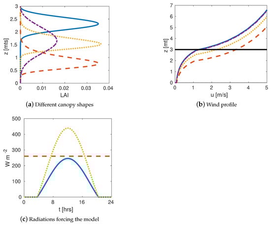
Figure 1. Inputs for the SHAW-derived model. (a) Different canopies shapes derived with the function $LAI\left(z\right)$ given by (13) and different combinations of the parameters pair $({\alpha }_c,{\beta }_c)$. Cases, 1 (solid), 2 (dashed), 3 (dotted), and 4 (dash-dot). (b) Zoom of the Wind-profile for the four canopies shape, the black line is the canopy height. (c) 24 h radiation forcing from the sky at the upper layer in the canopy, Short wave-direct (solid), Short wave-diffusive (dotted), and Long wave-direct (dashed).

Between the inputs of the model, we have the vertical wind profile computed by Equation (7) and displayed in Figure 1b, including the line $h_c$ = 3 m, and the radiation forcing on the top of the canopy and shown in Figure 1c. Concerning the vertical profile of the wind, hold the decreasing values within the canopy and the exponential beyond it, noting that the interchange resistance coefficients (6a) and (6b) depends on wind speed. For radiation, diffusive and direct shortwave radiations reach their maximum at midday and are zero at night time. Meanwhile, the longwave radiation is set to be constant throughout the day, as it is dependent of the sky temperature.

Before showing the spatial-time evolution of the state variables, Figure 2 shows an approach of the thermal energy change in the canopy computing as $\Delta E=m_c{c}_c(T_l-T_{a,ref})$. As expected, the maximum energy change is located where is the maximum foliage mass position from the soil and where the wind velocity is minimum, being Case 2, which both conditions hold (Figure 2b). In contrast, the minimum energy change is a consequence of a foliage mass upper located from the soil and faster wind. In Case 1, both conditions hold with almost zero change (Figure 2a). Additionally, in all canopies (Figure 2), the foliage mass quantity on its limits is so slight that the thermal energy change is practically zero. This leads us to expect maximum leaf temperatures and quick humidity saturation at canopies’ ends. However, these extremes values of temperature and humidity will be mitigated within the canopies. This is confirmed by the results explained and shown below.

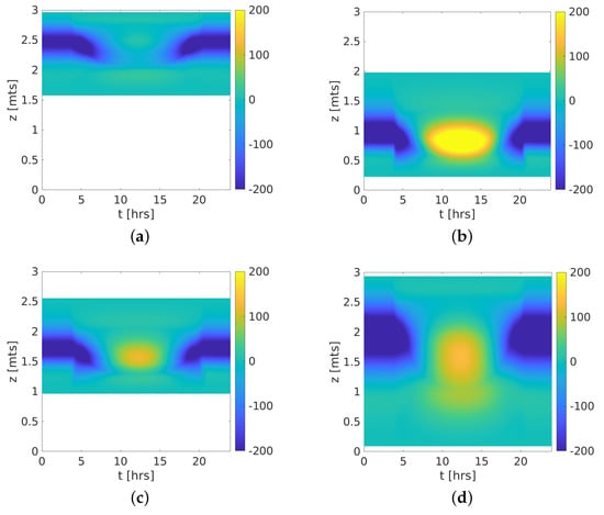
Figure 2. Energy change $\Delta E$ at 24 h for all canopy shapes. (a) Case 1; (b) Case 2; (c) Case 3; (d) Case 4.

We show in the following figures the space-time evolution of the state variables of the SHAW-derived model for all canopies. Numerical solutions have been computed in the mesh defined in Section 3 and a time interval of 24 h. As initial conditions to leaf-air-soil temperatures and leaf humidity were taken the outputs of a previous models’ run of four days.

For the leaf temperature, Cases 1, 2, and 3 are all characterized by maximum temperatures on canopy ends due to minimum foliage mass and forcing by radiation from sky and soil (see Figure 3a–c). In particular, Case 4 shows notably more forcing on the low end of the canopy, in consequence, showing notably more significant temperature change there (due to a small foliage mass and a very short distance to the soil that radiates longwave energy and reflects part of the short wave radiation due to its albedo). Inside the canopy, the foliage mass allows moderate temperatures due to a significant net heat capacity.

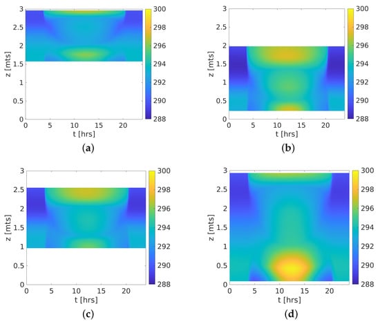
Figure 3. Leaf temperature variations at 24 h for all canopy shapes. (a) Case 1; (b) Case 2; (c) Case 3; (d) Case 4.

Now, the temperature of the air column is shown in Figure 4, taking only the part of the air column that matches the canopy height of 3 m. It is important to note that all canopies have the same temperature profile: maximum values close to the soil and decreasing through the canopy. We highlighted Case 2 (Figure 4a), which has a lower located foliage mass and higher energy change $\Delta E$ with air. In consequence, this canopy presents the maximum temperatures. Conforming the foliage mass is located in upper positions, the temperatures shown lower values due to a significant distance from the soil and less energy change capacity. Concerning Case 4, a well-mixed air temperature column (Figure 4d) is shown due to its height-wise foliage distribution. Nevertheless, all canopies show a scant variation (≈0.4 K). This could be partly due to a high reference wind velocity $u_{ref}$ = 10 m/s. To demonstrate that, we take lower velocity values $u_{ref}$ = 5 m/s and $u_{ref}$ = 2.5 m/s for Case 2, and results are shown in Figure 5a,b where a major variation (≈1 K) is observed. There are others factors than potentially influence too, such as the constant temperature $T_{a,ref}$ = 293.15 K imposed as boundary condition in the top of the air column and some parameters as the total biomass $m_{tot}$.

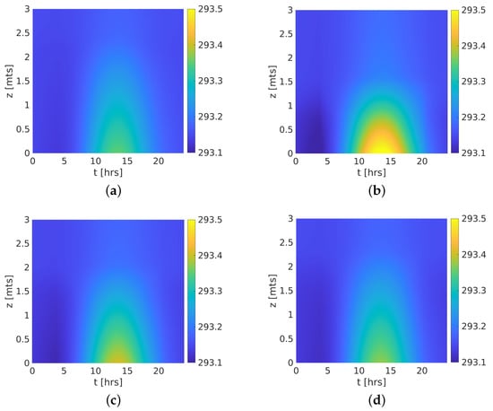
Figure 4. Air column temperatures at 24 h for all canopy shapes. (a) Case 1; (b) Case 2; (c) Case 3; (d) Case 4.

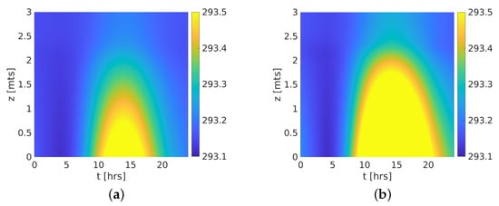
Figure 5. Wind velocity partly explains the scant variability of the temperature in the air column. Temperatures at 24 h for the canopy shape 2 subjected to different wind velocities. (a) Case 2 $u_{ref}$ = 5 m/s; (b) Case 2 $u_{ref}$ = 2.5 m/s.

About humidity, it is greatly influenced by the saturated soil (because of the more significant moisture flux in the soil-air inter-phase) is apparent the effect of the canopy shape, trapping, and adding (due to leaf stoma) humidity, avoiding its distribution along with the canopy. This can be observed clearly in opposites Cases 1 and 2 (Figure 6a,b) wherein the humidity line reaches 2.5 m in the first case, meanwhile only reaches 1.5 m in Case 1, matching with their respective canopies top.

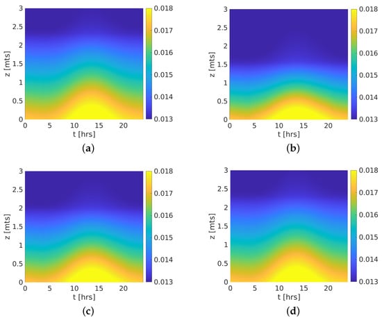
Figure 6. Leaf humidity at 24 h for all canopy shapes. (a) Case 1; (b) Case 2; (c) Case 3; (d) Case 4.

Finally, the soil temperature is computed from surface to a depth of −2 m but only presents a notable variation in a thick layer. Due to this, is shown only an average soil temperature. Then in Figure 7a is shown the average leaf temperature focuses our attention in the midday, wherein Case 2 (low foliage mass location) reaches the maximum temperature, opposite to its minimum corresponding to Case 1 (top foliage mass location). This indicates that to an upper location of the foliage, less soil temperature (due to a higher sensible heat soil cooling caused by steeper air and soil temperature difference).

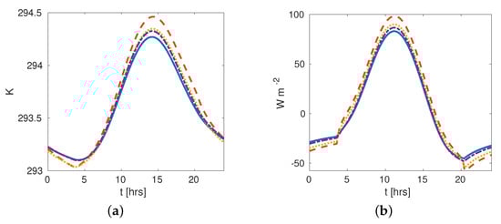
Figure 7. Temperature and heat balance in the soil, Cases 1 (solid), 2 (dashed), 3 (dotted), and 4 (dash-dot). In essence, the soil temperature and heat balance is the same for all the canopies, maximum values at midday and energy released at night. However, Cases 1 and 2 represent the extreme values from the rest of them. (a) Soil temperature (averaged in width); (b) Energy balance.

Of course, the model generates other interesting outputs: the net shortwave and longwave radiations in both soil and canopy. Energy fluxes at the soil surface (Equation (19c)) are shown in Figure 7b for all canopies. We expect that the canopy absorbs energy during the day and releases it at night. The shape canopy made a clear difference in magnitude of released-absorbed energy with all canopies having the same exposed behavior. We point out that at midday, a difference of 20 Wm⁻² between Cases 1 and 2, being the maximum and minimum values of the four cases.

4. Discussions

In this work, a SHAW-derived model was formulated and solved numerically with the finite element method, being an alternative to finite difference schemes used by Flerchinger et al. [7,8,9,10,11] and other authors (see reference list [28]). This new approach allows using irregular meshes and potentially scaling the model to a higher dimension which was possible thanks to the continuous vertical function LAI proposed in Section 2.2. Moreover, numerical solutions were derived by combining relaxed fix-point iterations (to address nonlinearity) and a time scheme of predicted-corrector type (to yield stability).

Typically, theoretical and experimental studies of heat and humidity fluxes in canopies are made on a fixed foliage profile either take it as a simple geometry shape —commonly triangular or rectangular— or derivate it by curve fitting of in situ measures. In this work, were compared different canopies characterized exclusively by their foliage profile or shape and analyzed their heat and water transport dynamics. Numerical results suggested that the canopy shape notably influences the vertical profile of leaf, air and soil temperatures, humidity and heat fluxes. Therefore, this work could be a first step in selecting a canopy tree to maximize its benefits. Examples could be several: windbreak, soil cooling or heating, reduced air temperature, maximized air humidity, covering the soil from radiation, and others. Furthermore, the simplicity of the Weibull distribution to characterize a canopy shape with only two parameters opens the possibility of formulating optimization problems related to minimizing harmful phenomenons.

We emphasize that the model could be sensitive to other canopy parameters: leaf width, orientation and diameter, stomata resistance, and specific heat capacity. Moreover, latitude, day of the year, and meteorological parameters are significant too. Therefore, changing these parameters would imply changes in the model outputs. However, address a model sensibility analysis would overextend this paper leaving it to future work.

A value-added of this work is a complete description of the mathematical methodology to obtain the numerical solution of the model, this could be attractive for researchers to reproduce results, update the model, or as another example of how to approach a nonlinear system of PDEs.

Finally, a comparison between the SHAW model and the SHAW-derived model (Equations (1a)–(1d)) could be interesting. However, there are essential differences between them: turbulent transport (K-theory), soil humidity, shape canopy characterization and numerical approach, which have been pointed out through the paper. Indeed, in [16] the substitution of the K-theory by the L-theory made a better approach of the modeled variables to the data. This motivates us to a model update for reach goals such as validation or model comparison. However, we do not consider this observations as a step backward but a direction for future work.

References

- Bonan, G.B.; Patton, E.G.; Finnigan, J.J.; Baldocchi, D.D.; Harman, I.N. Moving beyond the incorrect but useful paradigm: Reevaluating big-leaf and multilayer plant canopies to model biosphere-atmosphere fluxes—A review. Agric. For. Meteorol. 2021, 306, 108435. [Google Scholar] [CrossRef]
- Yun, S.H.; Park, C.Y.; Kim, E.S.; Lee, D.K. A Multi-Layer Model for Transpiration of Urban Trees Considering Vertical Structure. Forests 2020, 11, 1164. [Google Scholar] [CrossRef]
- Dargahi, M.; Newson, T.; Moore, J.R. A Numerical Approach to Estimate Natural Frequency of Trees with Variable Properties. Forests 2020, 11, 915. [Google Scholar] [CrossRef]
- Zhao, W.; Qualls, R.J. A multiple-layer canopy scattering model to simulate shortwave radiation distribution within a homogeneous plant canopy. Water Resour. Res. 2005, 41. [Google Scholar] [CrossRef]
- Wu, C.; Chau, K.; Huang, J. Modelling coupled water and heat transport in a soil–mulch–plant–atmosphere continuum (SMPAC) system. Appl. Math. Model. 2007, 31, 152–169. [Google Scholar] [CrossRef] [Green Version]
- Banimahd, S.; Zand-Parsa, S. Simulation of evaporation, coupled liquid water, water vapor and heat transport through the soil medium. Agric. Water Manag. 2013, 130, 168–177. [Google Scholar] [CrossRef]
- Flerchinger, G.; Pierson, F. Modeling plant canopy effects on variability of soil temperature and water. Agric. For. Meteorol. 1991, 56, 227–246. [Google Scholar] [CrossRef]
- Flerchinger, G.N.; Kustas, W.P.; Weltz, M.A. Simulating Surface Energy Fluxes and Radiometric Surface Temperatures for Two Arid Vegetation Communities Using the SHAW Model. J. Appl. Meteorol. 1998, 37, 449–460. [Google Scholar] [CrossRef] [Green Version]
- Flerchinger, G.; Yu, Q. Simplified expressions for radiation scattering in canopies with ellipsoidal leaf angle distributions. Agric. For. Meteorol. 2007, 144, 230–235. [Google Scholar] [CrossRef]
- Flerchinger, G.; Xiao, W.; Sauer, T.; Yu, Q. Simulation of within-canopy radiation exchange. NJAS-Wagening. J. Life Sci. 2009, 57, 5–15. [Google Scholar] [CrossRef] [Green Version]
- Flerchinger, G.N.; Reba, M.L.; Link, T.E.; Marks, D. Modeling temperature and humidity profiles within forest canopies. Agric. For. Meteorol. 2015, 213, 251–262. [Google Scholar] [CrossRef]
- Coops, N.C.; Smith, M.L.; Jacobsen, K.L.; Martin, M.; Ollinger, S. Estimation of plant and leaf area index using three techniques in a mature native eucalypt canopy. Austral Ecol. 2004, 29, 332–341. [Google Scholar] [CrossRef]
- Mori, S.; Hagihara, A. Crown profile of foliage area characterized with the Weibull distribution in a hinoki (Chamaecyparis obtusa) stand. Trees 1991, 5, 1432–2285. [Google Scholar] [CrossRef]
- Launiainen, S.; Katul, G.G.; Lauren, A.; Kolari, P. Coupling boreal forest CO2, H2O and energy flows by a vertically structured forest canopy–Soil model with separate bryophyte layer. Ecol. Model. 2015, 312, 385–405. [Google Scholar] [CrossRef]
- Campbell, G.S.; Norman, J. An Introduction to Environmental Biophysics; Springer Science + Business Media: New York, NY, USA, 1988. [Google Scholar] [CrossRef]
- Flerchinger, G.N.; Reba, M.L.; Marks, D. Measurement of Surface Energy Fluxes from Two Rangeland Sites and Comparison with a Multilayer Canopy Model. J. Hydrometeorol. 2012, 13, 1038–1051. [Google Scholar] [CrossRef]
- Absi, R. Reinvestigating the Parabolic-Shaped Eddy Viscosity Profile for Free Surface Flows. Hydrology 2021, 8, 126. [Google Scholar] [CrossRef]
- Harman, I.N.; Finnigan, J.J. Scalar Concentration Profiles in the Canopy and Roughness Sublayer. Bound.-Layer Meteorol. 2008, 129, 323–351. [Google Scholar] [CrossRef]
- Liu, R.; Huang, W.; Ren, H.; Yang, G.; Wang, J.; Li, X. Research on FPAR vertical distribution in different variety maize canopy. In Proceedings of the 2011 IEEE International Geoscience and Remote Sensing Symposium, Vancouver, BC, Canada, 24–29 July 2011; pp. 2745–2748. [Google Scholar] [CrossRef]
- Lazzari, L. 8-Statistical Analysis of Corrosion Data. In Engineering Tools for Corrosion; Lazzari, L., Ed.; European Federation of Corrosion (EFC) Series; Woodhead Publishing: Kidlington, UK, 2017; pp. 131–148. [Google Scholar] [CrossRef]
- Yang, X.; Witcosky, J.J.; Miller, D.R. Vertical Overstory Canopy Architecture of Temperate Deciduous Hardwood Forests in the Eastern United States. For. Sci. 1999, 45, 349–358. [Google Scholar] [CrossRef]
- Coops, N.C.; Hilker, T.; Wulder, M.A.; St-Onge, B.; Siggins, A.; Trofymow, J.A. Estimating canopy structure of Douglas-fir forest stands from discrete-return LiDAR. Trees 1999, 21, 349–358. [Google Scholar] [CrossRef] [Green Version]
- Oleson, K.W.; Lawrence, D.M.; Bonan, G.B.; Flanner, M.G.; Kluzek, E.; Lawrence, P.J.; Levis, S.; Swenson, S.C.; Thornton, P.E.; Dai, A.; et al. Technical Description of Version 4.0 of the Community Land Model (CLM); Technical Report; National Center for Atmospheric Research: Boulder, CO, USA, 2010. [Google Scholar]
- Larson, M.G.; Bengzon, F. The Finite Element Method: Theory, Implementation, and Applications; Springer: Berlin/Heidelberg, Germany, 2013. [Google Scholar] [CrossRef]
- Reddy, J.N. An Introduction to Nonlinear Finite Element Analysis with Applications to Heat Transfer, Fluid Mechanics, and Solid Mechanics, 2nd ed.; Oxford University Press: Oxford, UK, 2014. [Google Scholar] [CrossRef]
- Nakamura, S. Applied Numerical Methods with Software; Prentice-Hall: Harlow, UK, 1991; ISBN 9780130410474. [Google Scholar]
- Hansen, F.V. Surface Roghness Lengths; Technical Report; U.S. Army Research Laboratory: Adelphi, MD, USA, 1994. [Google Scholar]
- SHAW Model: USDA ARS. 2021. Available online: https://www.ars.usda.gov/ARSUserFiles/20520500/SHAW/302/SHAWReferences.pdf’ (accessed on 4 February 2021).
- Iqbal, M. An Introduction to Solar Radiation; Academic Press Canada: Waterloo, ON, Canada, 1983. [Google Scholar] [CrossRef]
- Zhao, W.; Qualls, R.J. Modeling of long-wave and net radiation energy distribution within a homogeneous plant canopy via multiple scattering processes. Water Resour. Res. 2006, 42. [Google Scholar] [CrossRef] [Green Version]
Publisher’s Note: MDPI stays neutral with regard to jurisdictional claims in published maps and institutional affiliations. |
© 2021 by the authors. Licensee MDPI, Basel, Switzerland. This article is an open access article distributed under the terms and conditions of the Creative Commons Attribution (CC BY) license (https://creativecommons.org/licenses/by/4.0/).