
Enlargement of the Field of View Based on Image Region Prediction Using Thermal Videos


Abstract
:1. Introduction
- -
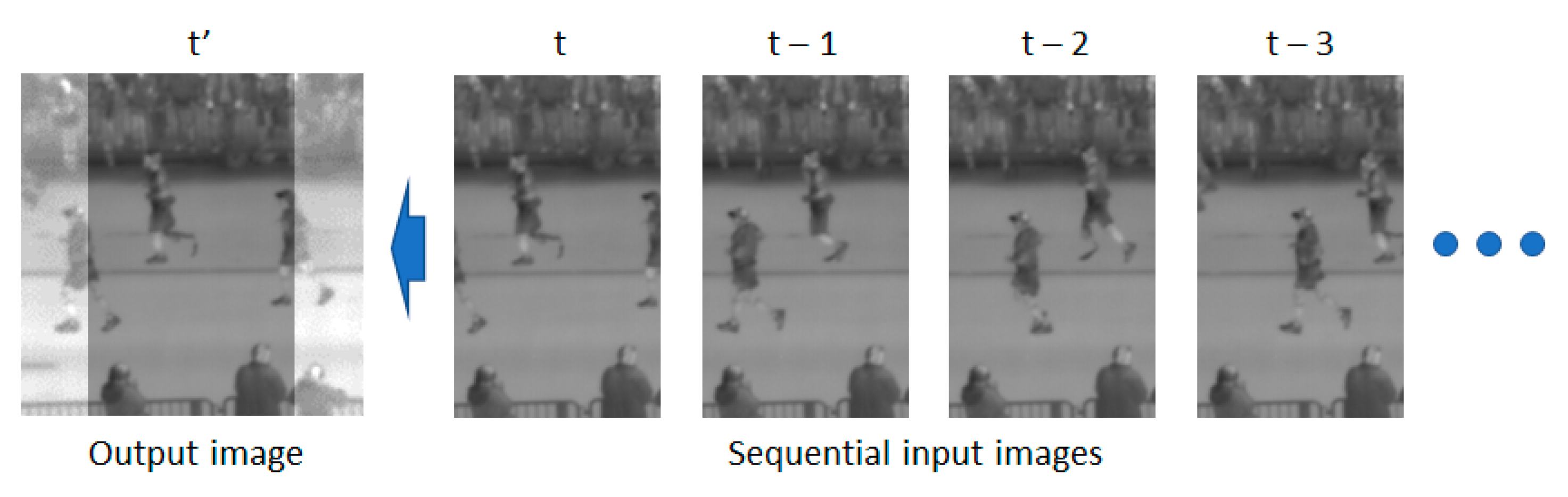
- For thermal camera images, in this study, image prediction was performed in which, for the first time, the occurrence of noise was minimized while wide regions to left and right sides of the FOV in the current image were accurately generated.
- -
- In this study, IPGAN-2 is proposed for performing image prediction.
- -
- For improving the accuracy of image prediction, binary images corresponding to sequential input thermal images were used as input for IPGAN-2.
- -
- The IPGAN-2 model proposed has been disclosed [16] for a fair performance evaluation by other researchers.
2. Related Works
2.1. Not Using Previous Frames but Using Current Frame (Image Inpainting)
2.2. Using Current and Previous Frames
2.2.1. Prediction of Next Frame
2.2.2. Prediction of Next Sequential Frames
2.2.3. Prediction of Small Left Region of Current Frame
3. Materials and Methods
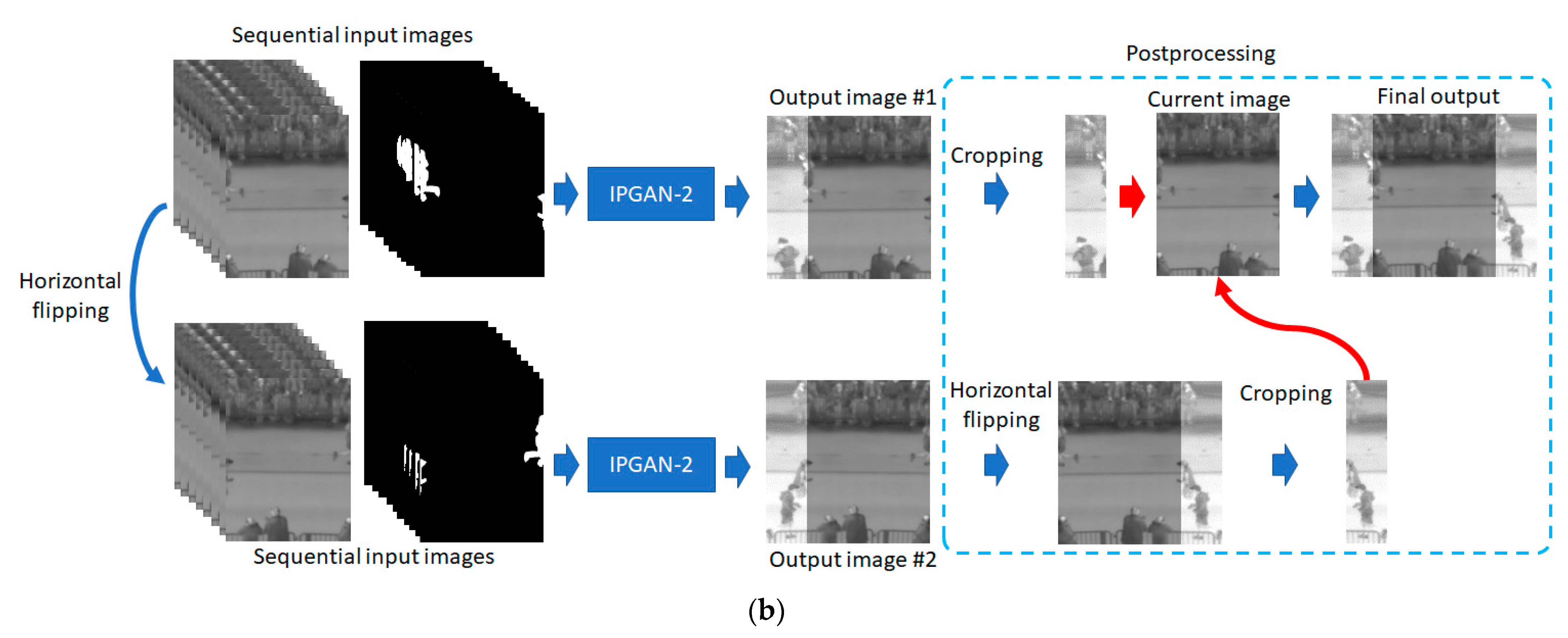
3.1. Overall Procedure of Proposed Method
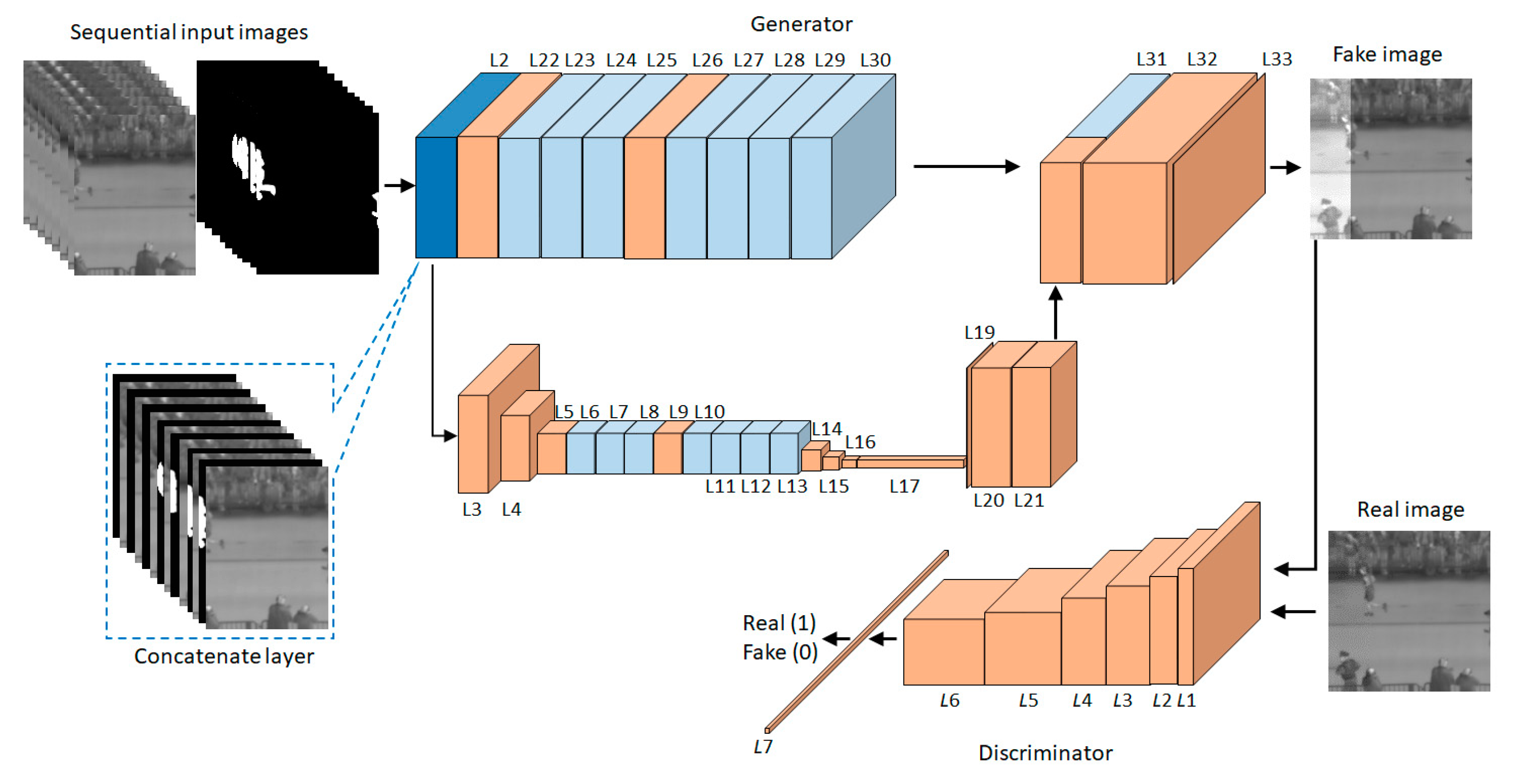
3.2. Proposed IPGAN-2 Model
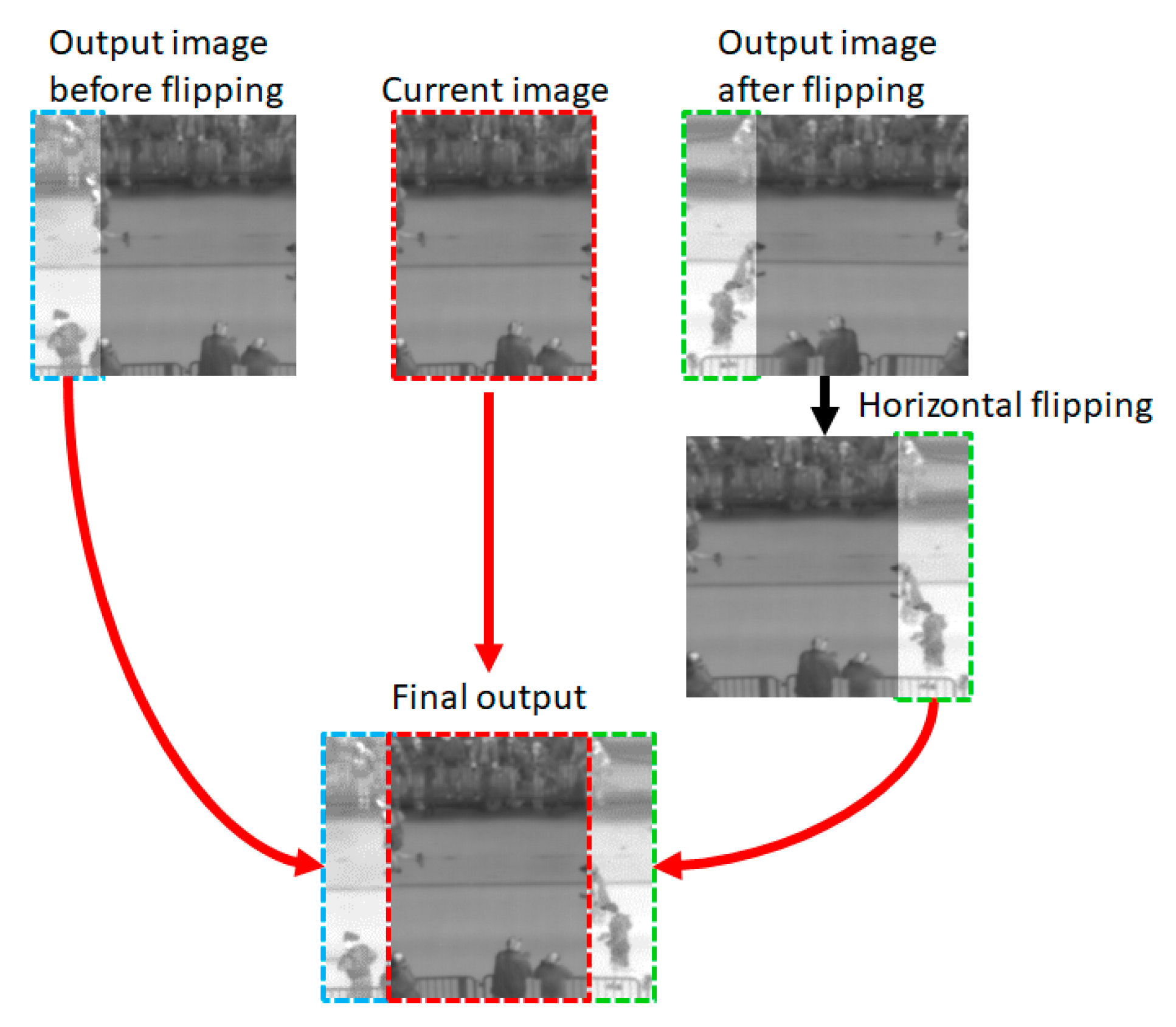
3.3. Postprocessing
3.4. Differences between IPGAN and Proposed IPGAN-2
3.5. Dataset and Experimental Setup
4. Results
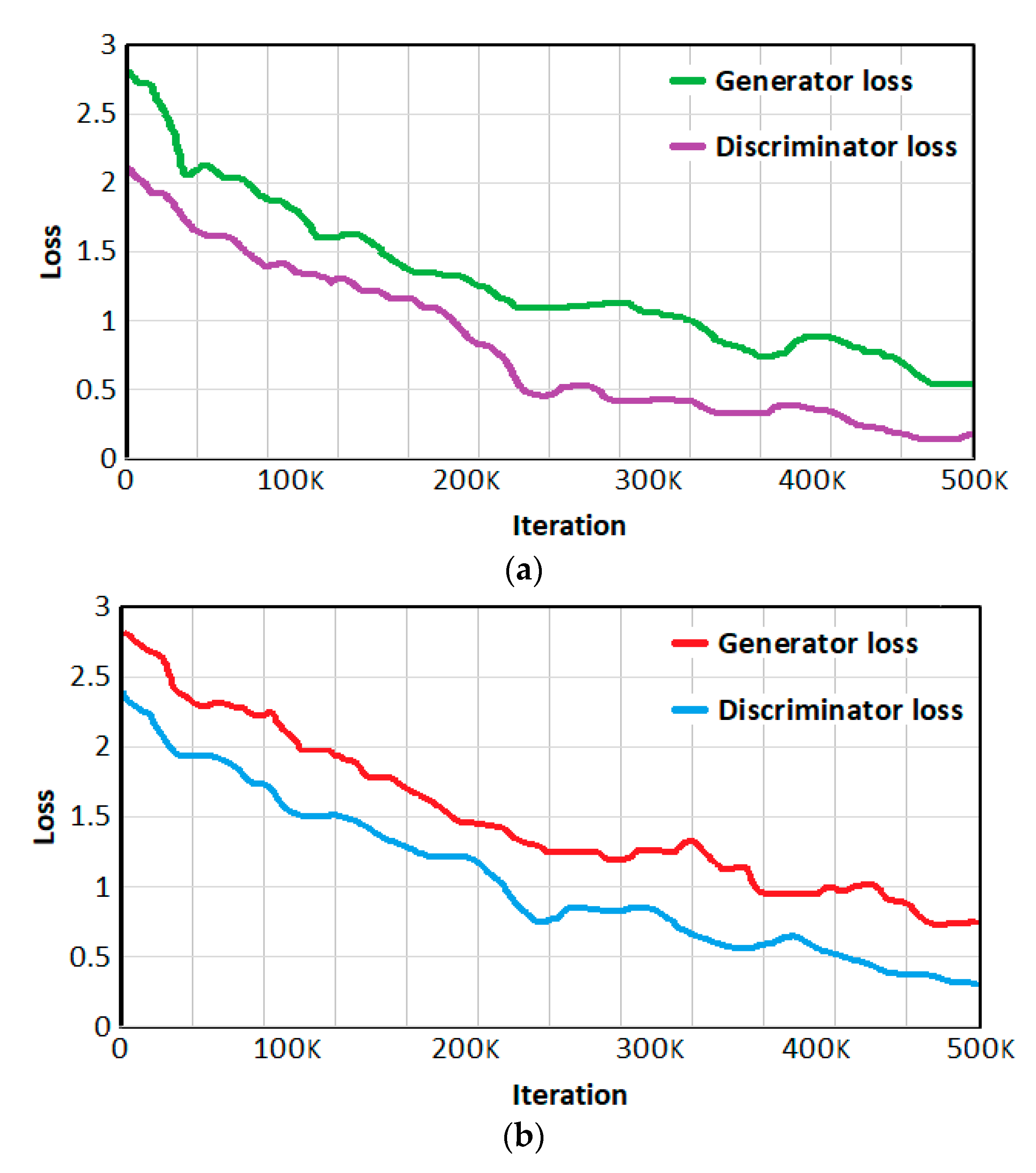
4.1. Training
4.2. Testing (Ablation Study)
4.3. Comparisons of Proposed Method with the State-of-the-Art Methods
4.4. Experiments Using Different Datasets (Casia Dataset C and BU-TIV Marathon Dataset) for Training and Testing
4.5. Processing Time
5. Discussion
6. Conclusions
Author Contributions
Funding
Institutional Review Board Statement
Informed Consent Statement
Data Availability Statement
Conflicts of Interest
References
- Gong, J.; Zhao, J.; Li, F.; Zhang, H. Vehicle detection in thermal images with an improved yolov3-tiny. In Proceedings of the IEEE International Conference on Power, Intelligent Computing and Systems, Shenyang, China, 28–30 July 2020. [Google Scholar]
- Batchuluun, G.; Kang, J.K.; Nguyen, D.T.; Pham, T.D.; Muhammad, A.; Park, K.R. Deep learning-based thermal image reconstruction and object detection. IEEE Access 2021, 9, 5951–5971. [Google Scholar] [CrossRef]
- Batchuluun, G.; Yoon, H.S.; Nguyen, D.T.; Pham, T.D.; Park, K.R. A study on the elimination of thermal reflections. IEEE Access 2019, 7, 174597–174611. [Google Scholar] [CrossRef]
- Batchuluun, G.; Baek, N.R.; Nguyen, D.T.; Pham, T.D.; Park, K.R. Region-based removal of thermal reflection using pruned fully convolutional network. IEEE Access 2020, 8, 75741–75760. [Google Scholar] [CrossRef]
- Zhang, X.; Chen, R.; Liu, G.; Li, X.; Luo, S.; Fan, X. Thermal infrared tracking using multi-stages deep features fusion. In Proceedings of the Chinese Control and Decision Conference, Hefei, China, 22–24 August 2020. [Google Scholar]
- Svanström, F.; Englund, C.; Alonso-Fernandez, F. Real-time drone detection and tracking with visible, thermal and acoustic sensors. In Proceedings of the 25th International Conference on Pattern Recognition, Milan, Italy, 10–15 January 2021. [Google Scholar]
- Liu, Q.; Li, X.; He, Z.; Fan, N.; Yuan, D.; Wang, H. Learning deep multi-level similarity for thermal infrared object tracking. IEEE Trans. Multimed. 2021, 23, 2114–2126. [Google Scholar] [CrossRef]
- Liu, Q.; He, Z.; Li, X.; Zheng, Y. PTB-TIR: A thermal infrared pedestrian tracking benchmark. IEEE Trans. Multimed. 2020, 22, 666–675. [Google Scholar] [CrossRef]
- Kang, B.; Liang, D.; Ding, W.; Zhou, H.; Zhu, W.-P. Grayscale-thermal tracking via inverse sparse representation-based collaborative encoding. IEEE Trans. Image Process. 2020, 29, 3401–3415. [Google Scholar] [CrossRef] [PubMed]
- Batchuluun, G.; Kim, Y.G.; Kim, J.H.; Hong, H.G.; Park, K.R. Robust behavior recognition in intelligent surveillance environments. Sensors 2016, 16, 1010. [Google Scholar] [CrossRef] [PubMed]
- Batchuluun, G.; Kim, J.H.; Hong, H.G.; Kang, J.K.; Park, K.R. Fuzzy system based human behavior recognition by combining behavior prediction and recognition. Expert Syst. Appl. 2017, 81, 108–133. [Google Scholar] [CrossRef]
- Batchuluun, G.; Nguyen, D.T.; Pham, T.D.; Park, C.; Park, K.R. Action recognition from thermal videos. IEEE Access 2019, 7, 103893–103917. [Google Scholar] [CrossRef]
- Batchuluun, G.; Kang, J.K.; Nguyen, D.T.; Pham, T.D.; Arsalan, M.; Park, K.R. Action recognition from thermal videos using joint and skeleton information. IEEE Access 2021, 9, 11716–11733. [Google Scholar] [CrossRef]
- Batchuluun, G.; Koo, J.H.; Kim, Y.H.; Park, K.R. Image region prediction from thermal videos based on image prediction generative adversarial network. Mathematics 2021, 9, 1053. [Google Scholar] [CrossRef]
- Wu, Z.; Fuller, N.; Theriault, D.; Betke, M. A thermal infrared video benchmark for visual analysis. In Proceedings of the IEEE Conference on Computer Vision and Pattern Recognition Workshops, Columbus, OH, USA, 23–28 June 2014. [Google Scholar]
- Image Prediction Generative Adversarial Network v2 (IPGAN-2). Available online: http://dm.dgu.edu/link.html (accessed on 25 March 2021).
- Liu, H.; Jiang, B.; Xiao, Y.; Yang, C. Coherent semantic attention for image inpainting. In Proceedings of the IEEE/CVF International Conference on Computer Vision Workshop, Seoul, Korea, 27 October–2 November 2019. [Google Scholar]
- Yu, J.; Lin, Z.; Yang, J.; Shen, X.; Lu, X.; Huang, T. Free-form image inpainting with gated convolution. In Proceedings of the IEEE/CVF International Conference on Computer Vision Workshop, Seoul, Korea, 27 October–2 November 2019. [Google Scholar]
- Shin, Y.-G.; Sagong, M.-C.; Yeo, Y.-J.; Kim, S.-W.; Ko, S.-J. PEPSI++: Fast and lightweight network for image inpainting. IEEE Trans. Neural Netw. Learn. Syst. 2021, 32, 252–265. [Google Scholar] [CrossRef] [PubMed] [Green Version]
- Pathak, D.; Krähenbühl, P.; Donahue, J.; Darrell, T.; Efros, A.A. Context encoders: Feature learning by inpainting. In Proceedings of the IEEE Conference on Computer Vision and Pattern Recognition, Las Vegas, NV, USA, 27–30 June 2016. [Google Scholar]
- Nazeri, K.; Ng, E.; Joseph, T.; Qureshi, F.; Ebrahimi, M. EdgeConnect: Structure guided image inpainting using edge prediction. In Proceedings of the IEEE/CVF International Conference on Computer Vision Workshop, Seoul, Korea, 27 October–2 November 2019. [Google Scholar]
- Elharrouss, O.; Almaadeed, N.; Al-Maadeed, S.; Akbari, Y. Image inpainting: A review. Neural Process. Lett. 2020, 51, 2007–2028. [Google Scholar] [CrossRef] [Green Version]
- Liang, X.; Lee, L.; Dai, W.; Xing, E.P. Dual motion GAN for future-flow embedded video prediction. In Proceedings of the IEEE International Conference on Computer Vision (ICCV), Venice, Italy, 22–29 October 2017. [Google Scholar]
- Sedaghat, N.; Zolfaghari, M.; Brox, T. Hybrid learning of optical flow and next frame prediction to boost optical flow in the wild. arXiv 2017, arXiv:1612.03777v2. [Google Scholar]
- Mahjourian, R.; Wicke, M.; Angelova, A. Geometry-based next frame prediction from monocular video. arXiv 2017, arXiv:1609.06377v2. [Google Scholar]
- Haziq, R.; Basura, F. A log-likelihood regularized KL divergence for video prediction with a 3D convolutional variational recurrent network. In Proceedings of the IEEE/CVF Winter Conference on Applications of Computer Vision Workshops, Virtual, Waikola, HI, USA, 5–9 January 2021. [Google Scholar]
- Guen, V.L.; Thome, N. Disentangling physical dynamics from unknown factors for unsupervised video prediction. In Proceedings of the IEEE Conference on Computer Vision and Pattern Recognition, Virtual, Seattle, WA, USA, 14–19 June 2020. [Google Scholar]
- Finn, C.; Goodfellow, I.; Levine, S. Unsupervised learning for physical interaction through video prediction. In Proceedings of the Advances in Neural Information Processing Systems 29, Barcelona, Spain, 5–10 December 2016. [Google Scholar]
- Xu, J.; Xu, H.; Ni, B.; Yang, X.; Darrell, T. Video prediction via example guidance. In Proceedings of the 37th International Conference on Machine Learning, Online, 13–18 July 2020. [Google Scholar]
- Babaeizadeh, M.; Finn, C.; Erhan, D.; Campbell, R.H.; Levine, S. Stochastic variational video prediction. In Proceedings of the 6th International Conference on Learning Representations, Vancouver, BC, Canada, 30 April–3 May 2018. [Google Scholar]
- Oprea, S.; Martinez-Gonzalez, P.; Garcia-Garcia, A.; Castro-Vargas, J.A.; Orts-Escolano, S.; Garcia-Rodriguez, J.; Argyros, A. A review on deep learning techniques for video prediction. IEEE Trans. Pattern Anal. Mach. Intell 2020. [Google Scholar] [CrossRef]
- Rasouli, A. Deep learning for vision-based prediction: A survey. arXiv 2020, arXiv:2007.00095v2. [Google Scholar]
- Nvidia GeForce GTX TITAN X. Available online: https://www.nvidia.com/en-us/geforce/products/10series/titan-x-pascal/ (accessed on 25 March 2021).
- OpenCV. Available online: http://opencv.org/ (accessed on 25 March 2021).
- Python. Available online: https://www.python.org/download/releases/ (accessed on 25 March 2021).
- Keras. Available online: https://keras.io/ (accessed on 25 March 2021).
- Kingma, D.P.; Ba, J.L. Adam: A method for stochastic optimization. arXiv 2014, arXiv:1412.6980. [Google Scholar]
- Peak Signal-to-Noise Ratio. Available online: https://en.wikipedia.org/wiki/Peak_signal-to-noise_ratio (accessed on 29 April 2021).
- Wang, Z.; Bovik, A.C.; Sheikh, H.R.; Simoncelli, E.P. Image quality assessment: From error visibility to structural similarity. IEEE Trans. Image Process. 2004, 13, 600–612. [Google Scholar] [CrossRef] [Green Version]
- Powers, D.M.W. Evaluation: From precision, recall and f-measure to ROC, informedness, markedness & correlation. Mach. Learn. Technol. 2011, 2, 37–63. [Google Scholar]
- Derczynski, L. Complementarity, f-score, and NLP evaluation. In Proceedings of the International Conference on Language Resources and Evaluation, Portorož, Slovenia, 23–28 May 2016. [Google Scholar]
- He, K.; Gkioxari, G.; Dollár, P.; Girshick, R. Mask R-CNN. In Proceedings of the IEEE International Conference on Computer Vision, Venice, Italy, 22–29 October 2017. [Google Scholar]
- Tan, D.; Huang, K.; Yu, S.; Tan, T. Efficient night gait recognition based on template matching. In Proceedings of the 18th International Conference on Pattern Recognition, Hong Kong, China, 20–24 August 2006. [Google Scholar]
- Selvaraju, R.R.; Cogswell, M.; Das, A.; Vedantam, R.; Parikh, D.; Batra, D. Grad-CAM: Visual explanations from deep networks via gradient-based localization. arXiv 2016, arXiv:1610.02391v4. [Google Scholar]


| Category | Not Using Previous Frames but Using Current Frame (Prediction of Removed Part in Current Frame (Image in painting)) | Using Current and Previous Frames | |||
|---|---|---|---|---|---|
| Prediction of Next Frame | Prediction of Next Sequential Frames | Prediction of Small Left Region of Current Frame | Prediction of Large Right and Left Regions of Current Frame | ||
| Methods | CSA layer [17], gated convolution + SN-PatchGAN [18], PEPSI [19], context encoder [20], edge prediction and image completion [21], and review [22] | ConvLSTMGAN [23], OptCNN-Hybrid [24], ConvLSTM [25] | Encoder–decoder model [26,29], PhyDNet [27], CNN + LSTM [28], SV2P [30], and review & survey [31,32] | IPGAN [14] | IPGAN-2 (Proposed method) |
| Input | High-quality and high-resolution RGB visible light image | Low-quality and low-resolution grayscale thermal image | Low-quality and low-resolution grayscale thermal image and binary image | ||
| Output | RGB visible light image | An RGB thermal image | A grayscale thermal image | ||
| Advantages | High performance is achieved by restoring the information deleted in the current image by using the remaining information of the current image. | High performance is obtained when generating the next image by using the current image and previous sequential images. |
|
| |
| Disadvantages |
|
| Low processing speed | ||
| Input thermal image with size of (120 × 160 × 1) = Input binary image with size of (120 × 160 × 1) = Output thermal image with size of (160 × 160 × 1) = Final output thermal image with size of (200 × 160 × 1) = IPGAN-2 model = Horizontal image flipping = Image cropping = | |
| Algorithm procedure | Output shape/dimension |
| | |
| Layer Number | Layer Type | Number of Filters | Number of Parameters | Layer Connection (Connected to) |
|---|---|---|---|---|
| 0 | input_layers_1–20 | 0 | input_1–20 | |
| 1 | input_layers_21–40 | 0 | input_21–40 | |
| 2 | concat_1 | 0 | input_layers_1–20 & input_layers_21–40 | |
| 3 | encod_block_1 | 64 | 48,640 | concat_1 |
| 4 | encod_block_2 | 64 | 73,984 | encod_block_1 |
| 5 | encod_block_3 | 64 | 73,984 | encod_block_2 |
| 6 | res_block_1 | 64 | 73,920 | encod_block_3 |
| 7 | res_block_2 | 64 | 73,920 | res_block_1 |
| 8 | res_block_3 | 64 | 73,920 | res_block_2 |
| 9 | conv_block_1 | 128/64 | 147,840 | res_block_3 |
| 10 | res_block_4 | 64 | 73,920 | conv_block_1 |
| 11 | res_block_5 | 64 | 73,920 | res_block_4 |
| 12 | res_block_6 | 64 | 73,920 | res_block_5 |
| 13 | res_block_7 | 64 | 73,920 | res_block_6 |
| 14 | encod_block_4 | 64 | 73,984 | res_block_7 |
| 15 | encod_block_5 | 64 | 73,984 | encod_block_4 |
| 16 | encod_block_6 | 64 | 73,984 | encod_block_5 |
| 17 | conv2d_1 | 3200 | 1,846,400 | encod_block_6 |
| 18 | prelu_1 | 3200 | 3200 | |
| 19 | reshape | 0 | conv2d_1 | |
| 20 | conv2d_2 | 64 | 640 | reshape |
| 21 | conv2d_3 | 64 | 36,928 | conv2d_2 |
| 22 | conv_block_2 | 128/64 | 97,152 | concat_1 |
| 23 | res_block_8 | 64 | 73,920 | conv_block_2 |
| 24 | res_block_9 | 64 | 73,920 | res_block_8 |
| 25 | res_block_10 | 64 | 73,920 | res_block_9 |
| 26 | conv_block_3 | 128/64 | 147,840 | res_block_10 |
| 27 | res_block_11 | 64 | 73,920 | conv_block_3 |
| 28 | res_block_12 | 64 | 73,920 | res_block_11 |
| 29 | res_block_13 | 64 | 73,920 | res_block_12 |
| 30 | res_block_14 | 64 | 73,920 | res_block_13 |
| 31 | concat_2 | 0 | conv2d_3 & res_block_14 | |
| 32 | conv2d_4 | 256 | 147,712 | concat_2 |
| 33 | conv2d_5 | 1 | 2305 | conv2d_4 |
| 34 | tanh | 0 | conv2d_5 | |
| Total number of trainable parameters: 3,883,457 | ||||
| Layer Number | Layer Type | Number of Filters | Layer Connection (Connected to) |
|---|---|---|---|
| 1 | conv2d_1 | 64 | input |
| 2 | prelu_1 | 64 | conv2d_1 |
| 3 | conv2d_2 | 64 | prelu_1 |
| 4 | prelu_2 | 64 | conv2d_2 |
| 5 | maxpool | prelu_2 |
| Layer Number | Layer Type | Number of Filters | Layer Connection (Connected to) |
|---|---|---|---|
| 1 | conv2d_1 | 128 | input |
| 2 | prelu_1 | 128 | conv2d_1 |
| 3 | conv2d_2 | 64 | prelu_1 |
| 4 | prelu_2 | 64 | conv2d_2 |
| Layer Number | Layer Type | Number of Filters | Layer Connection (Connected to) |
|---|---|---|---|
| 1 | conv2d_1 | 64 | input |
| 2 | prelu | 64 | conv2d_1 |
| 3 | conv2d_2 | 64 | prelu |
| 4 | add | conv2d_2 & input |
| Layer Number | Layer Type | Number of Filters | Number of Parameters | Layer Connection (Connected to) |
|---|---|---|---|---|
| 0 | input layer | 0 | input | |
| 1 | conv_block_1 | 32 | 896 | input layer |
| 2 | conv_block_2 | 64 | 18,496 | conv_block_1 |
| 3 | conv_block_3 | 128 | 73,856 | conv_block_2 |
| 4 | conv_block_4 | 128 | 147,584 | conv_block_3 |
| 5 | conv_block_5 | 256 | 295,168 | conv_block_4 |
| 6 | conv_block_6 | 256 | 590,080 | conv_block_5 |
| 7 | dense | 92,417 | conv_block_6 | |
| 8 | sigmoid | 0 | dense | |
| Total number of trainable parameters: 1,218,497 | ||||
| Layer Number | Layer Type | Layer Connection (Connected to) |
|---|---|---|
| 1 | conv2d | input |
| 2 | lrelu | conv2d |
| Steps | Previous Method [14] (IPGAN) | Proposed Method (IPGAN-2) |
|---|---|---|
| Input | Original thermal image (85 × 170 × 1) | Original thermal image (120 × 160 × 1) |
| Preprocessing | Conversion of original thermal image to three-channel color thermal image with zero padding | Image binarization by using background subtraction and horizontal flipping |
| Network input | Three-channel color thermal image (170 × 170 × 3) | Original thermal image (120 × 160 × 1) and binary image (120 × 160 × 1) |
| Network output | Three-channel color thermal image (170 × 170 × 3) | One-channel thermal image (160 × 160 × 1) |
| Postprocessing | Image cropping (crop a small part of predicted region) and combining | Image cropping (crop the entire predicted region), horizontal flipping, and combining |
| Output | Three-channel color thermal image (105 × 170 × 3) | One-channel thermal image (200 × 160 × 1) |
| Factors | Previous Method [14] (IPGAN) | Proposed Method (IPGAN-2) |
|---|---|---|
| Predicted region | Only left side | Left and right sides |
| Size of predicted region | Smaller (input of 85 × 170 to output of 105 × 170) | Larger (input of 120 × 160 to output of 200 × 160) |
| Error | Gray noise occurs over predicted region | No gray noise |
| Processing speed | Higher | Lower |
| Parameters | Weight Decay (Weight Regularization L2) | Loss | Kernel Initializer | Bias Initializer | Optimizer | Learning Rate | Beta_1 | Beta_2 | Epsilon | Iterations | Batch Size |
|---|---|---|---|---|---|---|---|---|---|---|---|
| Search Space | [0.001, 0.01, 0.1] | [“binary cross-entropy loss”, “mse”,“VGG-19 loss”] | “glorot uniform” | “zeros” | [“SGD”, “adam”] | [0.0001, 0.001, 0.01, 0.1] | [0.7, 0.8, 0.9] | [0.8, 0.9, 0.999] | [1 × 10⁻⁹, 1 × 10⁻⁸, 1 × 10⁻⁷] | [1~500 K] | [1,4,8] |
| Selected Value | 0.01 | “binary cross-entropy loss” | “glorot uniform” | “zeros” | “adam” | 0.001 | 0.9 | 0.999 | 1 × 10⁻⁸ | 483,581 | 1 |
| Methods | PSNR | SSIM |
|---|---|---|
| pred2reg | 19.450 | 0.8156 |
| predWholeIm | 14.501 | 0.6395 |
| 2-chanPred | 15.261 | 0.6121 |
| singImPred | 19.214 | 0.8132 |
| seq&sing | 21.340 | 0.8413 |
| pred3-chan [14] | 24.927 | 0.8403 |
| predLreg | 26.592 | 0.9581 |
| Methods | TPR | PPV | F1 | ACC | IoU |
|---|---|---|---|---|---|
| or-detect | 0.601 | 0.613 | 0.606 | 0.71 | 0.483 |
| pred-detect (proposed) | 0.887 | 0.847 | 0.866 | 0.914 | 0.730 |
| Methods | Image Prediction | Mask R-CNN | |||||
|---|---|---|---|---|---|---|---|
| PSNR | SSIM | TPR | PPV | F1 | ACC | IoU | |
| Haziq et al. [26] | 22.843 | 0.8917 | 0.801 | 0.654 | 0.720 | 0.904 | 0.521 |
| Liu et al. [17] | 20.557 | 0.8454 | 0.638 | 0.626 | 0.631 | 0.864 | 0.432 |
| Shin et al. [19] | 22.181 | 0.8781 | 0.687 | 0.631 | 0.657 | 0.866 | 0.502 |
| Nazeri et al. [21] | 22.112 | 0.8724 | 0.651 | 0.672 | 0.661 | 0.890 | 0.514 |
| pred3-chan [14] | 25.146 | 0.8711 | 0.792 | 0.714 | 0.753 | 0.901 | 0.536 |
| Proposed method | 26.018 | 0.9437 | 0.887 | 0.847 | 0.866 | 0.914 | 0.730 |
| Results | Image Prediction | Mask R-CNN | |||||
|---|---|---|---|---|---|---|---|
| PSNR | SSIM | TPR | PPV | F1 | ACC | IoU | |
| Fold-1 | 24.984 | 0.9211 | 0.851 | 0.821 | 0.835 | 0.895 | 0.725 |
| Fold-2 | 24.028 | 0.9064 | 0.835 | 0.802 | 0.818 | 0.889 | 0.705 |
| Average | 24.506 | 0.9137 | 0.843 | 0.811 | 0.826 | 0.892 | 0.715 |
| Methods | Component | Processing Time |
|---|---|---|
| Image prediction | IPGAN-2 (before flipping) | 48.4 |
| IPGAN-2 (after flipping) | 48.4 | |
| Postprocessing | 0.01 | |
| Human segmentation | Mask R-CNN | 54.1 |
| Total | 150.91 | |
Publisher’s Note: MDPI stays neutral with regard to jurisdictional claims in published maps and institutional affiliations. |
© 2021 by the authors. Licensee MDPI, Basel, Switzerland. This article is an open access article distributed under the terms and conditions of the Creative Commons Attribution (CC BY) license (https://creativecommons.org/licenses/by/4.0/).
Share and Cite
Batchuluun, G.; Baek, N.R.; Park, K.R. Enlargement of the Field of View Based on Image Region Prediction Using Thermal Videos. Mathematics 2021, 9, 2379. https://doi.org/10.3390/math9192379
Batchuluun G, Baek NR, Park KR. Enlargement of the Field of View Based on Image Region Prediction Using Thermal Videos. Mathematics. 2021; 9(19):2379. https://doi.org/10.3390/math9192379
Chicago/Turabian StyleBatchuluun, Ganbayar, Na Rae Baek, and Kang Ryoung Park. 2021. "Enlargement of the Field of View Based on Image Region Prediction Using Thermal Videos" Mathematics 9, no. 19: 2379. https://doi.org/10.3390/math9192379
APA StyleBatchuluun, G., Baek, N. R., & Park, K. R. (2021). Enlargement of the Field of View Based on Image Region Prediction Using Thermal Videos. Mathematics, 9(19), 2379. https://doi.org/10.3390/math9192379