Quantum-Like Sampling

Abstract

Probability theory is built around Kolmogorov’s axioms. To each event, a numerical degree of belief between 0 and 1 is assigned, which provides a way of summarizing the uncertainty. Kolmogorov’s probabilities of events are added, the sum of all possible events is one. The numerical degrees of belief can be estimated from a sample by its true fraction. The frequency of an event in a sample is counted and normalized resulting in a linear relation. We introduce quantum-like sampling. The resulting Kolmogorov’s probabilities are in a sigmoid relation. The sigmoid relation offers a better importability since it induces the bell-shaped distribution, it leads also to less uncertainty when computing the Shannon’s entropy. Additionally, we conducted 100 empirical experiments by quantum-like sampling 100 times a random training sets and validation sets out of the Titanic data set using the Naïve Bayes classifier. In the mean the accuracy increased from $78.84\%$ to $79.46\%$.

1. Introduction

Quantum algorithms are based on different principles than classical algorithm. Here we investigate a simple quantum-like algorithm that is motivated by quantum physics. The incapability between Kolmogorov’s probabilities and quantum probabilities results from the different norms that are used. In quantum probabilities the length of the vector in $l_2$ norm representing the amplitudes of all events is one. Usually, Kolmogorov’s probabilities are converted in Quantum-like probabilities by the squared root operation, it is difficult to attach any meaning to the squared root operation. Motivated by the lack of interpretability we define quantum-like sampling, the $l_2$ sampling. The resulting Kolmogorov’s probabilities are not any more linear but related to the sigmoid function. In the following we will introduce the traditional $l_1$ sampling Then we will introduce the quantum-like sampling, the $l_2$ sampling. We will indicate the relation between the $l_2$ sampling, the sigmoid function and the normal distribution. The quantum-like sampling leads to less uncertainty. We fortify this hypothesis by empirical experiments with a simple Naïve Bayes classifier on the Titanic dataset.

2. Kolmogorovs Probabilities

Probability theory is built around Kolmogorov’s axioms (first published in 1933 [1]). All probabilities are between 0 and 1. For any proposition x,

$$0\le p\left(x\right)\le 1$$

and

$$p\left(true\right)=1,p\left(false\right)=0.$$

To each sentence, a numerical degree of belief between 0 and 1 is assigned, which provides a way of summarizing the uncertainty. The last axiom expresses the probability of disjunction and is given by

$$p(x\vee y)=p\left(x\right)+p\left(y\right)-p(x\wedge y)$$

where do these numerical degrees of belief come from?

• Humans can believe in a subjective viewpoint, which can be determined by some empirical psychological experiments. This approach is a very subjective way to determine the numerical degree of belief.
• For a finite sample we can estimate the true fraction. We count the frequency of an event in a sample. We do not know the true value because we cannot access the whole population of events. This approach is called frequentist.
• It appears that the true values can be determined from the true nature of the universe, for example, for a fair coin, the probability of heads is $0.5$. This approach is related to the Platonic world of ideas. However, we can never verify whether a fair coin exists.

Frequentist Approach and $l_1$ Sampling

Relying on the frequentist approach, one can determine the probability of an event x by counting. If $\Omega$ is the set of all possible events, $p(\Omega )=1$ and the cardinality $\mathrm{card}(\Omega )$ determines the number of elements of a set $\Omega$ and $\mathrm{card}\left(x\right)$ is the number of elements of the set x and with $x\in \Omega$

$$p\left(x\right)=\frac{\mathrm{card}\left(x\right)}{\mathrm{card}(\Omega )}.$$

(1)

This kind of sampling is the $l_1$ sampling. With n events $x_1,x_2,...,x_n$ that describe all possible events of the set $\Omega$,

$$0\le \frac{\mathrm{card}\left(x_i\right)}{\mathrm{card}(\Omega )},\sum _{i=1}^n\frac{\mathrm{card}\left(x_i\right)}{\mathrm{card}(\Omega )}=1\iff \sum _{i=1}^n\mathrm{card}\left(x_i\right)=\mathrm{card}(\Omega )$$

We can interpret $\frac{\mathrm{card}\left({\omega }_i\right)}{\mathrm{card}(\Omega )}$ as dimension of an n dimensional vector with the vector being

$$\left(\begin{array}{c}\frac{\mathrm{card}\left(x_1\right)}{\mathrm{card}(\Omega )}\\ \frac{\mathrm{card}\left(x_2\right)}{\mathrm{card}(\Omega )}\\ \cdots \\ \frac{\mathrm{card}\left(x_n\right)}{\mathrm{card}(\Omega )}\end{array}\right).$$

(2)

with the $l_1$ norm

$${\parallel \mathbf{x}\parallel }_1=|x_1|+|x_2|+\cdots +|x_n|$$

(3)

it is as a unit-length vector in the norm $l_1$

$$\left|\frac{\mathrm{card}\left(x_1\right)}{\mathrm{card}(\Omega )}\right|+\left|\frac{\mathrm{card}\left(x_2\right)}{\mathrm{card}(\Omega )}\right|+\cdots +\left|\frac{\mathrm{card}\left(x_n\right)}{\mathrm{card}(\Omega )}\right|=1.$$

(4)

3. Quantum Probabilities

Quantum physics evaluates a probability $p\left(x\right)$ of a state x as the squared magnitude of a probability amplitude $A\left(x\right)$, which is represented by a complex number

$$p\left(x\right)={\left|A\left(x\right)\right|}^2=A{\left(x\right)}^{*}·A\left(x\right).$$

(5)

This is because the product of complex number with its conjugate is always a real number. With

$$A\left(x\right)=\alpha +\beta ·i$$

(6)

$$A{\left(x\right)}^{*}·A\left(x\right)=(\alpha -\beta ·i)·(\alpha +\beta ·i)$$

(7)

$$A{\left(x\right)}^{*}·A\left(x\right)={\alpha }^2+{\beta }^2={\left|A\left(x\right)\right|}^2.$$

(8)

Quantum physics by itself does not offer any justification or explanation beside the statement that it just works fine, see [2]. This quantum probabilities are as well called von Neumann probabilities. Converting two amplitudes into probabilities leads to an interference term $2·\Re (A\left(x\right)·A^{*}\left(y\right))$,

$$\begin{array}{c}\hfill {|A\left(x\right)+A\left(y\right)|}^2={\left|A\left(x\right)\right|}^2+{\left|A\left(y\right)\right|}^2+2·\Re (A\left(x\right)·A^{*}\left(y\right))\\ \hfill {|A\left(x\right)+A\left(y\right)|}^2=p\left(x\right)+p\left(y\right)+2·\Re (A\left(x\right)·A^{*}\left(y\right)),\end{array}$$

(9)

making both approaches, in general, incompatible

$${|A\left(x\right)+A\left(y\right)|}^2\ne p\left(x\right)+p\left(y\right).$$

(10)

In other words, the summation rule of classical probability theory is violated, resulting in one of the most fundamental laws of quantum mechanics, see [2]. In quantum physics we interpret $A\left(x_i\right)$ as dimension of an n dimensional vector with the vector being

$$\left(\begin{array}{c}A\left(x_1\right)\\ A\left(x_2\right)\\ \cdots \\ A\left(x_n\right)\end{array}\right).$$

(11)

In quantum physics the unit-length vector is computed in the in the norm $l_2$

$${\parallel \mathbf{x}\parallel }_2=\sqrt{\left(|x_1{|}^2+|x_2{|}^2+\cdots +{\left|x_n\right|}^2\right)}$$

(12)

instead of the norm $l_1$ with a unit-length vector in the norm $l_2$

$$|A\left(x_1\right){|}^2+|A\left(x_2\right){|}^2+\cdots +{\left|A\left(x_n\right)\right|}^2=1.$$

(13)

By replacing the $l_1$ norm by the Euclidean $l_2$ norm in the classical probability theory (Kolmogorov probabilities), we obtain quantum mechanics [3] with all the corresponding laws. The incapability between the Kolmogorov’s probabilities and quantum probabilities results from the simple fact

$${\parallel \mathbf{x}\parallel }_2\le {\parallel \mathbf{x}\parallel }_1.$$

(14)

This incapability is as well the basis for quantum cognition. Quantum cognition is motivated by clues from psychology indicate that human cognition is based on quantum probability rather than the traditional probability theory as explained by Kolmogorov’s axioms, see [4,5,6,7]. Empirical findings show that, under uncertainty, humans tend to violate the expected utility theory and consequently the laws of classical probability theory (e.g., the law of total probability [6,7,8]), In [4,9,10,11,12,13,14] leading to what is known as the “disjunction effect” which, in turn, leads to violation of the Sure Thing Principle. The violation results from an additional interference that influences the classical probabilities.

Conversion

The amplitude is the root of the belief multiplied with the corresponding phase [11,12,13] $\theta \in [0,2·\pi )$

$$A\left(x\right)=a(x,\theta )=\sqrt{p\left(x\right)}·e^{i·\theta }.$$

(15)

With $l_1$ sampling it is difficult to attach any meaning to $\sqrt{\mathrm{card}\left(x\right)}$,

$$a(x,\theta )=\sqrt{\frac{\mathrm{card}\left(x\right)}{\mathrm{card}(\Omega )}}·e^{i·\theta }.$$

(16)

Motivated by the lack of interpretability we define the quantum-like sampling, the $l_2$ sampling with n events $x_1,x_2,...,x_n$ that describe all possible events

$$\Phi =|\mathrm{card}\left(x_1\right){|}^2+|\mathrm{card}\left(x_2\right){|}^2+\cdots +{\left|\mathrm{card}\left(x_n\right)\right|}^2$$

(17)

$$p\left(x_i\right)=\frac{|\mathrm{card}\left(x_i\right){|}^2}{\Phi },\sum _{i=1}^n\frac{|\mathrm{card}\left({\omega }_i\right){|}^2}{\Phi }=1$$

(18)

and

$$a(x,\theta )=\frac{\mathrm{card}\left(x\right)}{\sqrt{\mathrm{card}(\Phi )}}·e^{i·\theta }.$$

(19)

with

$$\Omega \le \Phi \le {\Omega }^2.$$

(20)

The $l_2$ sampling leads to an interpretation of the amplitudes as a normalized frequency of occurrence of an event multiplied by the phase. $\Phi$ is dependent on the distribution of all values $\mathrm{card}\left(x_i\right)$. When developing empirical experiments that are explained by quantum cognition models $l_2$ sampling should be used rather than $l_1$ sampling. What is the interpretation of $|\mathrm{card}\left(x_i\right){|}^2$ outside quantum interpretation?

4. Quantum-Like Sampling and the Sigmoid Function

To understand the difference between $l_1$ sampling and $l_2$ sampling (quantum-like sampling) we will analyze a simple binary event x

$$p\left(x\right)+p(\neg x)=1.$$

For $l_1$ sampling $p\left(x\right)$ and $p(\neg x)$ is defined as

$$p\left(x\right)=\frac{\mathrm{card}\left(x\right)}{\mathrm{card}(\Omega )},p(\neg x)=\frac{\Omega -\mathrm{card}\left(x\right)}{\mathrm{card}(\Omega )}$$

and for $l_2$ sampling

$$p\left(x\right)=\frac{\mathrm{card}{\left(x\right)}^2}{\mathrm{card}{\left(x\right)}^2+{(\Omega -\mathrm{card}\left(x\right))}^2},p(\neg x)=\frac{{(\Omega -\mathrm{card}\left(x\right))}^2}{\mathrm{card}{\left(x\right)}^2+{(\Omega -\mathrm{card}\left(x\right))}^2}.$$

with

$$\omega =\mathrm{card}\left(x\right)$$

we can define the functions for binary $l_1$ and $l_2$ sampling as

$$f\left(\omega \right)=\frac{\omega }{\Omega }$$

(21)

and

$$g\left(\omega \right)=\frac{{\omega }^2}{{\omega }^2+{(\Omega -\omega )}^2},$$

(22)

In Figure 1 $f\left(\omega \right)=\frac{\omega }{\Omega }$ is compared to $g\left(\omega \right)=\frac{{\omega }^2}{{\omega }^2+{(\Omega -\omega )}^2}$ for $\Omega$, (a) $\Omega =4$, (b) $\Omega =10$, (c) $\Omega =100$ and (d) $\Omega =1000$. With growing size of $\Omega$ the function $g\left(\omega \right)$ converge to a continuous sigmoid function. In Figure 2 the sigmoid function $g\left(x\right)$ with $\Omega =10$ is compared to the well known scaled to the logistic function.

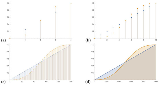
Figure 1. $f\left(\omega \right)=\frac{\omega }{\Omega }$ compared to $g\left(\omega \right)=\frac{{\omega }^2}{{\omega }^2+{(\Omega -\omega )}^2}$ for $\Omega$, (a) $\Omega =4$, (b) $\Omega =10$, (c) $\Omega =100$ and (d) $\Omega =1000$. With growing size of $\Omega$ the function $g\left(x\right)$ converge to a sigmoid function.

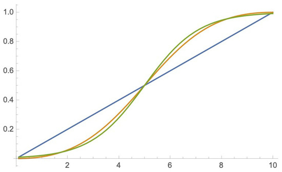
Figure 2. Sigmoid functions: $g\left(x\right)=\frac{x^2}{x^2+{(10-x)}^2}$ versus logistic function $\sigma \left(x\right)=\frac{1}{1+e^{-0.9523·(x-5)}}$.

The derivative of the sigmoid function $g\left(x\right)$ is a bell-shaped function. For the continuous function $g\left(x\right)$, the derivative is similar to the Gaussian distribution. The central limit theorem states that under certain (fairly common) conditions, the sum of many random variables will have an approximately Gausssian distribution. In Figure 3 the derivative of $g\left(x\right)=\frac{x^2}{x^2+{(10-x)}^2}$ with $\Omega =10$, $g^{\prime }\left(x\right)=-\frac{5(-10+x)x}{{(50-10x+x^2)}^2}$ is indicated and compared to Gaussian distribution $\mathcal{N}$ with $\mu =5$ and ${\sigma }^2=1.9^2$.

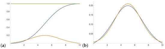
Figure 3. (a) $g\left(x\right)=\frac{x^2}{x^2+{(10-x)}^2}$ and $g^{\prime }\left(x\right)=-\frac{5(-10+x)x}{{(50-10x+x^2)}^2}$; (b) $g^{\prime }\left(x\right)=-\frac{5(-10+x)x}{{(50-10x+x^2)}^2}$ versus $\mathcal{N}\left(x\right|5,1.9^2)=\frac{1}{1.9\ast \sqrt{2\ast \pi }}·e^{-\frac{1}{2}·{\left(\frac{x-5}{1.9}\right)}^2}$.

The derivative of the sigmoid function $g\left(\omega \right)$ is less similar to the probability mass function of the the binomial distribution.

The $l_2$ sampling leads to natural sigmoid representation of probabilities that reflects the nature of Gaussian/Normal distribution. This leads to less uncertainty using $l_2$ compared to $l_1$ sampling represented by Shannon’s entropy.

$$H=-p\left(x\right)·{log}_{2}p\left(x\right)-p(\neg x)·{log}_{2}p(\neg x)$$

(23)

as can be seen in Figure 4 for $\Omega =100$.

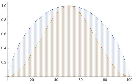
Figure 4. Shannon’s entropy H with $\Omega =100$, blue discrete plot for $l_1$ sampling and yellow discrete plot $l_2$ sampling.

Combination

Depending on $l_1$ or $l_2$ sampling we get different results when we combine probabilities. Multiplying two independent sampled events x and y results in the joint distribution

$$p_{l1}(x,y)=\frac{x}{10}·\frac{y}{10}$$

(24)

when $l_1$ sampled with $\Omega =10$ and

$$p_{l2}(x,y)=\frac{x^2}{x^2+{(10-x)}^2}·\frac{y^2}{y^2+{(10-y)}^2}$$

(25)

when $l_2$ sampled with $\Omega =10$ as indicated in the Figure 5. The same applies for weighted sum of information, corresponding to the Shannon’s entropy as used in the $ID3$ algorithm [15,16,17] for symbolical machine learning to preform a greedy search for small decision trees. Computing

$$H_{l1}=-\frac{x}{10}·{log}_2\frac{x}{10}-\frac{10-x}{10}·{log}_2\frac{10-x}{10}-\frac{y}{10}·{log}_2\frac{y}{10}-\frac{10-y}{10}·{log}_2\frac{10-y}{10}$$

(26)

when $l_1$ sampled with $\Omega =10$ and

$$H_{l2}=-\frac{x^2}{x^2+{(10-x)}^2}·{log}_2\frac{x^2}{x^2+{(10-x)}^2}-$$

$$\left(1-\frac{x^2}{x^2+{(10-x)}^2}\right)·{log}_2\left(1-\frac{x^2}{x^2+{(10-x)}^2}\right)-$$

$$\frac{x^2}{x^2+{(10-x)}^2}·{log}_2\frac{x^2}{x^2+{(10-x)}^2}-$$

$$\left(1-\frac{x^2}{x^2+{(10-x)}^2}\right)·{log}_2\left(1-\frac{x^2}{x^2+{(10-x)}^2}\right)$$

(27)

when $l_2$ sampled with $\Omega =10$ leads to different $H_1$ and $H_2$ values as indicated in the Figure 6.

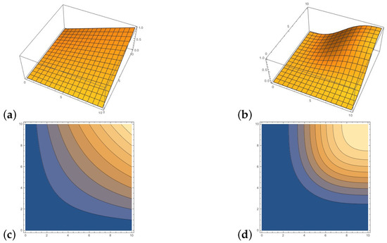
Figure 5. Multiplying two independent sampled events x and y with $\Omega =10$ leads to different results: (a) $p_{l1}(x,y)$, (b) $p_{l2}(x,y)$, (c) counterplot of $p_{l1}(x,y)$, (d) counterplot of $p_{l2}(x,y)$.

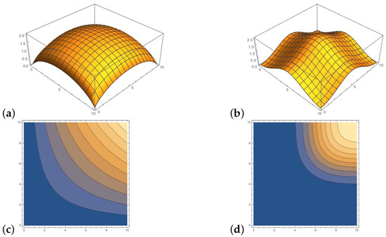
Figure 6. Different $H_1$ and $H_2$ values for sampled events x and y with $\Omega =10$: (a) $H_1(x,y)$, (b) $H_2(x,y)$, (c) counterplot of $H_1(x,y)$, (d) counterplot of $H_2(x,y)$.

Less uncertainty would lead to better results in machine learning. We preform empirical experiments with a simple Naïve Bayes classifier to fortify this hypothesis.

5. Naïve Bayes Classifier

For a target function $f:X\to h$, where each instance x described by attributes $a_1,a_2\cdots a_n$ Most probable value of $f\left(x\right)$ is:

$$h_{map}=arg\underset{h_i}{max}p\left(h_i\right|a_1,a_2,a_3,..,a_n)=\frac{p(a_1,a_2,a_3,...,a_n|h_i)·P\left(h_i\right)}{P(a_1,a_2,a_3,...,a_n)}$$

The likelihood of the conditional probability $p(a_1,a_2,a_3,...,a_n|h_i)$ is described by $2^n$ possible combinations. For n possible variables, the exponential growth of combinations being true or false becomes an intractable problem for large n since all $2^n-1$ possible combinations must be known. The decomposition of large probabilistic domains into weakly connected subsets via conditional independence,

$$p(a_1,a_2,a_3,...,a_n|h_i)=\prod _{j=1}^{n}p\left(a_j\right|h_i).$$

is known as the Naïve Bayes assumption and is one of the most important developments in the recent history of Artificial Intelligence [16]. It assumes that a single cause directly influences a number of events, all of which are conditionally independent. The Naïve Bayes classifier is defined as

$$h_{map}=arg\underset{h_i}{max}\prod _{j=1}^{n}P\left(a_j\right|h_i)·P\left(h_i\right).$$

Titanic Dataset

When the Titanic sank it killed 1502 out of 2224 passengers and crew. We are using a file titanic.cvs processed file from https://gist.github.com/michhar/ accessed on 1 July 2021 that corresponds to the file train.cvs from kaggle https://www.kaggle.com/c/titanic/data?select=train.csv accessed on 1 July 2021 that contains data for 891 of the real Titanic passengers. Each row represents one person. The columns describe different attributes about the person including their $PassengerId$, whether they $Survived$, heir passenger-class $Pclass$, their $Name$, their $Sex$, their $Age$, and other six attributes, see Figure 7. In our experiment we will only use the attributes $Survived$, $Pclass$, $Sex$ and $Age$.

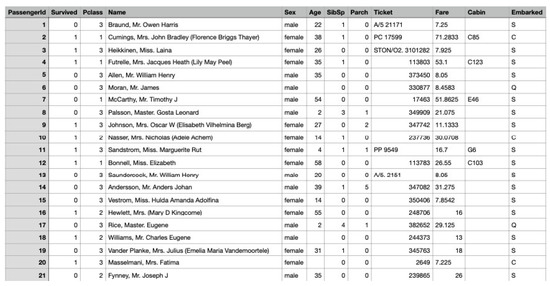
Figure 7. The Titanic data set is represented in an Excel table that contains data for 891 of the real Titanic passengers, some entries are not defined.

The binary attribute $Survived$ (=s) will be our target h resulting in the prior $p\left(s\right)$ and $p(\neg s)$. Out of the 891 passengers 342 survived and 549 did not survive. The attribute $Pclass$ has three values 1 for upper class, 2 for middle class and 3 for lower class. It will be binarized into the attribute c indicating if the person had a lower class cabin by

$$c=1ifPclass==3elsec=0,$$

in the case $Pclass$ is not defined the default value is 0. The attribute $Sex$ has two binary values represented by the binary attribute m

$$m=1ifSex==maleelsem=0,$$

in the case $Sex$ is not defined the default value is 0. The attribute $Age$ will be binarized into the attribute g indicating if the person is a child or grown up by

$$g=0ifAge<18elseg=1,$$

in the case $Age$ is not defined the default value is 1.

Using the $l_1$ sampling over the whole data set we get the values for the priors

$$p\left(s\right)=0.3838,p(\neg s)=0.6162,$$

and for the likelihoods,

$$p\left(c\right|s)=0.3480,p(\neg c\left|s\right)=0.6520,p\left(c\right|\neg s)=0.6776,p(\neg c|\neg s)=0.3224,$$

$$p\left(m\right|s)=0.3187,p(\neg m\left|s\right)=0.6813,p\left(m\right|\neg s)=0.8525,p(\neg m|\neg s)=0.14755,$$

$$p\left(g\right|s)=0.8216,p(\neg g\left|s\right)=0.178363,p\left(g\right|\neg s)=0.9053,p(\neg g|\neg s)=0.0947.$$

Using the $l_2$ sampling over the whole data set we get the values for the priors

$$p\left(s\right)=0.27957406,p(\neg s)=0.72042594$$

and for the likelihoods,

$$p\left(c\right|s)=0.2217,p(\neg c\left|s\right)=0.7783,p\left(c\right|\neg s)=0.8154,p(\neg c|\neg s)=0.1846,$$

$$p\left(m\right|s)=0.1796,p(\neg m\left|s\right)=0.8524,p\left(m\right|\neg s)=0.9709,p(\neg m|\neg s)=0.0291,$$

$$p\left(g\right|s)=0.95499,p(\neg g\left|s\right)=0.04501,p\left(g\right|\neg s)=0.9892,p(\neg g|\neg s)=0.0108.$$

The sampled probability values are quite different.

We measure the accuracy of our algorithm by dividing the number of entries it correctly classified by the total number of entries. For $l_1$ sampling there 190 are entries wrong classified resulting in the accuracy of $78.66\%$, for the $l_2$ sampling 179 entries are wrong classified resulting in the accuracy of $79.91\%$.

In the next step we separate our data set in a training set and a validation set resulting in 295 elements in the validation set We use sklearn.model_selection accessed on 1 July 2021 import train_test_split accessed on 1 July 2021 with the parameters train_test_split(XH,yy,test_size=0.33,random_state=42) accessed on 1 July 2021. The later is used to validate how well our algorithm is doing. For $l_1$ sampling 60 entries are wrong classified resulting in the accuracy of $79.66\%$, for the $l_2$ sampling 55 entries are wrong classified resulting in the accuracy of $81.36\%$.

In the next we sample the 100 times a random training set and validation set We use sklearn.model_selection accessed on 1 July 2021 import train_test_split accessed on 1 July 2021 with the parameters train_test_split(XH,yy,test_size=0.33) accessed on 1 July 2021. For $l_1$ sampling there were in the mean $62.42$ entries wrong classified resulting in the accuracy of $78.84\%$, for the $l_2$ sampling there were $60.59$ entries wrong classified resulting in the accuracy of $79.46\%$.

The trend from this simple evaluation indicates that $l_2$ sampling leads to better results compared to $l_1$ sampling in the empirical experiments.

So far we looked at the performance of classification models in terms of accuracy. Specifically, we measured error based on the fraction of mistakes. However, in some tasks, there are some types of mistakes that are worse than others. However in our simple task the correctly classified results when $l_1$ sampled are also correctly classified when $l_2$ sampled.

6. Conclusions

We introduced quantum-like sampling also called the $l_2$ sampling. The $l_2$ sampling leads to an interpretation of the amplitudes as a normalized frequency of occurrence of an event multiplied by the phase

$$a(x,\theta )=\frac{\mathrm{card}\left(x\right)}{\sqrt{\mathrm{card}(\Phi )}}·e^{i·\theta },$$

$\Phi$ is dependent on the distribution of all values $\mathrm{card}\left(x_i\right)$. When developing empirical experiments that are explained by quantum cognition models $l_2$ sampling should be used rather than $l_1$ sampling.

The quantum inspired $l_2$ sampling maps the probability values to a natural continuous sigmoid function, its derivative is is a bell-shaped function that is similar to the Gaussian distribution of events. The $l_2$ sampling improves the classification accuracy in machine learning models that are based on sampling as indicated by empirical experiments with Naïve Bayes classifier.

References

- Kolmogorov, A. Grundbegriffe der Wahrscheinlichkeitsrechnung; Springer: Berlin, Germany, 1933. [Google Scholar]
- Binney, J.; Skinner, D. The Physics of Quantum Mechanics; Oxford University Press: Oxford, UK, 2014. [Google Scholar]
- Aaronson, S. Is quantum mechanics an island in theoryspace? In Proceedings of the Växjö Conference Quantum Theory: Reconsideration of Foundations; Khrennikov, A., Ed.; University Press: Vaxjo, Sweden, 2004; Volume 10, pp. 15–28. [Google Scholar]
- Busemeyer, J.; Wang, Z.; Trueblood, J. Hierarchical bayesian estimation of quantum decision model parameters. In Proceedings of the 6th International Symposium on Quantum Interactions, Paris, France, 27–29 June 2012; pp. 80–89. [Google Scholar]
- Busemeyer, J.R.; Trueblood, J. Comparison of quantum and bayesian inference models. In Quantum Interaction; Lecture Notes in Computer, Science; Bruza, P., Sofge, D., Lawless, W., van Rijsbergen, K., Klusch, M., Eds.; Springer: Berlin/Heidelberg, Germany, 2009; Volume 5494, pp. 29–43. [Google Scholar]
- Busemeyer, J.R.; Wang, Z.; Lambert-Mogiliansky, A. Empirical comparison of markov and quantum models of decision making. J. Math. Psychol. 2009, 53, 423–433. [Google Scholar] [CrossRef]
- Busemeyer, J.R.; Wang, Z.; Townsend, J.T. Quantum dynamics of human decision-making. J. Math. Psychol. 2006, 50, 220–241. [Google Scholar] [CrossRef]
- Khrennikov, A. Quantum-like model of cognitive decision making and information processing. J. Biosyst. 2009, 95, 179–187. [Google Scholar] [CrossRef] [PubMed]
- Busemeyer, J.; Pothos, E.; Franco, R.; Trueblood, J. A quantum theoretical explanation for probability judgment errors. J. Psychol. Rev. 2011, 118, 193–218. [Google Scholar] [CrossRef] [PubMed] [Green Version]
- Busemeyer, J.; Wang, Z. Quantum cognition: Key issues and discussion. Top. Cogn. Sci. 2014, 6, 43–46. [Google Scholar] [CrossRef] [PubMed]
- Wichert, A. Principles of Quantum Artificial Intelligence: Quantum Problem Solving and Machine Learning, 2nd ed.; World Scientific: Singapore, 2020. [Google Scholar]
- Wichert, A.; Moreira, C. Balanced quantum-like model for decision making. In Proceedings of the 11th International Conference on Quantum Interaction, Nice, France, 3–5 September 2018; pp. 79–90. [Google Scholar]
- Wichert, A.; Moreira, C.; Bruza, P. Quantum-like bayesian networks. Entropy 2020, 22, 170. [Google Scholar] [CrossRef] [PubMed] [Green Version]
- Yukalov, V.; Sornette, D. Decision theory with prospect interference and entanglement. Theory Decis. 2011, 70, 283–328. [Google Scholar] [CrossRef] [Green Version]
- Luger, G.F.; Stubblefield, W.A. Artificial Intelligence, Structures and Strategies for Complex Problem Solving, 3rd ed.; Addison-Wesley: Boston, MA, USA, 1998. [Google Scholar]
- Mitchell, T. Machine Learning; McGraw-Hill: New York, NY, USA, 1997. [Google Scholar]
- Winston, P.H. Artificial Intelligence, 3rd ed.; Addison-Wesley: Boston, MA, USA, 1992. [Google Scholar]
Publisher’s Note: MDPI stays neutral with regard to jurisdictional claims in published maps and institutional affiliations. |
© 2021 by the author. Licensee MDPI, Basel, Switzerland. This article is an open access article distributed under the terms and conditions of the Creative Commons Attribution (CC BY) license (https://creativecommons.org/licenses/by/4.0/).